Tensor Product Multiscale Many-Particle Spaces with ... - ULB Bonn

Tensor Product Multiscale Many-Particle Spaces with Finite-Order Weights for the Electronic Schrödinger Equation

Dissertation zur Erlangung des Doktorgrades (Dr. rer. nat.) der Mathematisch–Naturwissenschaftlichen Fakultät der Rheinischen Friedrich–Wilhelms–Universität Bonn

vorgelegt von Jan Hamaekers aus Neuwied Bonn 2009

Angefertigt mit Genehmigung der Mathematisch–Naturwissenschaftlichen Fakultät der Rheinischen Friedrich–Wilhelms–Universität Bonn

1. Referent: Prof. Dr. Michael Griebel 2. Referent: Prof. Dr. Helmut Harbrecht Tag der Promotion: 20.07.2009 Erscheinungsjahr: 2009 Diese Dissertation ist auf dem Hochschulschriftenserver der ULB Bonn http://hss.ulb.uni-bonn.de/diss_online online elektronisch publiziert.

Zusammenfassung In der vorliegenden Arbeit beschäftigen wir uns mit gewichteten Tensorprodukt-Multiskalen-Mehrteilchen-Approximationsräumen und deren Anwendung zur numerischen Lösung der elektronischen Schrödinger-Gleichung. Aufgrund der hohen Problemdimension ist eine direkte numerische Lösung der elektronischen Schrödinger-Gleichung mit Standard-Diskretisierungsverfahren zur linearen Approximation unmöglich, weshalb üblicherweise Monte Carlo Methoden (VMC/DMC) oder nichtlinearen Modellapproximationen wie Hartree-Fock (HF), Coupled Cluster (CC) oder Dichtefunktionaltheorie (DFT) verwendet werden. In dieser Arbeit wird eine numerische Methode auf Basis von adaptiven dünnen Gittern und einer teilchenweisen Unterraumzerlegung bezüglich Einteilchenfunktionen aus einer nichtlinearen Rang-1 Approximation entwickelt und für parallele Rechnersysteme implementiert. Dünne Gitter vermeiden die in der Dimension exponentielle Komplexität üblicher Diskretisierungsmethoden und führen zu einem konvergenten numerischen Ansatz mit garantierter Konvergenzrate. Zudem enhalten unsere zugrunde liegenden gewichteten Mehrteilchen Tensorprodukt-Multiskalen-Approximationsräume die bekannten Configuration Interaction (CI) Räume als Spezialfall. Zur Konstruktion unseres Verfahrens führen wir zunächst allgemeine MehrteilchenSobolevräume ein, welche die Standard-Sobolevräume sowie Sobolevräume mit dominierender gemischter Glattheit beinhalten. Wir analysieren die Approximationseigenschaften und schätzen Konvergenzraten und Kostenkomplexitätsordungen in Abhängigkeit der Glattheitsparameter und Abfalleigenschaften ab. Mit Hilfe bekannter Regularitätseigenschaften der elektronischen Wellenfunktion ergibt sich, dass die Konvergenzrate bis auf logarithmische Terme unabhängig von der Zahl der Elektronen und fast identisch mit der Konvergenzrate im Fall von zwei Elektronen ist. Neben der Rate spielt allerdings die Abhängigkeit der Konstanten in der Kostenkomplexität von der Teilchenzahl eine wichtige Rolle. Basierend auf Zerlegungen des Einteilchenraumes konstruieren wir eine Unterraumzerlegung des Mehrteilchenraumes, welche insbesondere die bekannte ANOVAZerlegung, die HDMR-Zerlegung sowie die CI-Zerlegung als Spezialfälle beinhaltet. Eine zusätzliche Gewichtung der entsprechenden Unterräume mit Gewichten von endlicher Ordnung q führt zu Mehrteilchenräumen, in denen sich das Approximationsproblem einer N -Teilchenfunktion zu Approximationsproblemen von q-Teilchenfunktionen reduziert. Mit dem Ziel, Konstanten möglichst kleiner Größe bezüglich der Kostenkomplexität zu erhalten, stellen wir ein heuristisches adaptives Verfahren zur Konstruktion einer Sequenz von endlich-dimensionalen Unterräumen eines gewichteten Mehrteilchen-Tensorprodukt-Multiskalen-Approximationsraumes vor. Außerdem konstruieren wir einen Frame aus Multiskalen-Gauss-Funktionen und verwenden Einteilchenfunktionen im Rahmen der Rang-1 Approximation in der Form von Gauss- und modulierten-Gauss-Funktionen. Somit können die zur Aufstellung der Matrizen des zugehörigen diskreten Eigenwertproblems benötigten Ein- und Zweiteilchenintegrale analytisch berechnet werden. Schließlich wenden wir unsere Methode auf kleine Atome und Moleküle mit bis zu sechs Elektronen (18 Raumdimensionen) an. Die numerischen Resultate zeigen, dass sich die aus der Theorie zu erwartenden Konvergenzraten auch praktisch ergeben.

Danksagung An dieser Stelle möchte ich die Gelegenheit nutzen, um allen Personen zu danken, die mich bei dieser Arbeit unterstützt haben. Dieser Dank gilt zunächst Prof. Dr. Michael Griebel für die interessante Promotionsthematik, die vielen wertvollen Ideen und hilfreichen Diskussionen, aber auch für die Bereitstellung von exzellenten Arbeitsbedingungen. Ebenfalls möchte ich mich bei Prof. Dr. Helmut Harbrecht für die Übernahme des Zweitgutachtens bedanken. Ein herzlicher Dank gebührt Christian Feuersänger, Margrit Klitz und Ralf Wildenhues für die große Hilfe beim Korrekturlesen der Arbeit. Abschließend möchte ich meinen Kollegen am Institut für Numerische Simulation meinen Dank für das freundliche und inspirierende Arbeitsklima aussprechen. Bonn, im Mai 2009

Jan Hamaekers

Für Zeynep und Felix Can

Contents 1 Introduction

1

2 Sobolev Spaces for Many-Particle Functions 2.1 Preliminaries . . . . . . . . . . . . . . . . . . . . . . . . . . . . . . . 2.1.1 Notation . . . . . . . . . . . . . . . . . . . . . . . . . . . . . . 2.1.2 Fourier transform . . . . . . . . . . . . . . . . . . . . . . . . . 2.1.3 Regularity and decay . . . . . . . . . . . . . . . . . . . . . . . 2.2 Many-particle Sobolev spaces . . . . . . . . . . . . . . . . . . . . . . 2.3 Hyperbolic cross approximation . . . . . . . . . . . . . . . . . . . . . 2.3.1 Multiscale decomposition of general hyperbolic cross spaces . 2.3.2 Approximation by general sparse grid spaces . . . . . . . . . 2.4 Weighted many-particle spaces . . . . . . . . . . . . . . . . . . . . . 2.4.1 Particle-wise subspace splitting . . . . . . . . . . . . . . . . . 2.4.2 Many-particle spaces with finite-order weights . . . . . . . . . 2.5 Symmetric and antisymmetric many-particle spaces . . . . . . . . . . 2.5.1 Symmetric and antisymmetric general sparse grid spaces . . . 2.5.2 Particle-wise splitting of symmetric and antisymmetric spaces 2.6 Summary . . . . . . . . . . . . . . . . . . . . . . . . . . . . . . . . .

. . . . . . . . . . . . . . .

. . . . . . . . . . . . . . .

. . . . . . . . . . . . . . .

9 9 9 11 12 12 16 19 22 32 33 37 40 44 46 49

3 Electronic Schrödinger Equation 3.1 Born-Oppenheimer approximation . . . . . . . . 3.2 Antisymmetry principle . . . . . . . . . . . . . . 3.3 Variational formulation . . . . . . . . . . . . . . . 3.4 Properties of the solution . . . . . . . . . . . . . 3.4.1 Discrete spectrum and exponential bounds 3.4.2 Cusp conditions and regularity results . . 3.4.3 Decay of weak mixed derivatives . . . . . 3.5 Summary . . . . . . . . . . . . . . . . . . . . . .

. . . . . . . .

. . . . . . . .

. . . . . . . .

51 51 52 55 57 57 59 63 70

. . . . . . .

73 73 74 78 79 80 83 89

4 Numerical Methods 4.1 Galerkin discretization . . . . . . . . . . . . . . 4.1.1 Löwdin rules . . . . . . . . . . . . . . . 4.1.2 Parallel eigenvalue solvers . . . . . . . . 4.2 Multiscale Gaussian frame . . . . . . . . . . . . 4.2.1 Gaussians in multiresolution analysis . . 4.2.2 One-particle multiscale Gaussian frame . 4.2.3 Many-particle Gaussian frame . . . . . .

. . . . . . .

. . . . . . . . . . . . . . .

. . . . . . . . . . . . . . .

. . . . . . . . . . . . . . .

. . . . . . . . . . . . . . .

. . . . . . . . . . . . . . .

. . . . . . . . . . . . . . .

. . . . . . . . . . . . . . .

. . . . . . . . . . . . . . .

. . . . . . . . . . . . . . .

. . . . . . . . . . . . . . .

. . . . . . . . . . . . . . .

. . . . . . .

. . . . . . .

i

Contents 4.3 4.4 4.5

Approximation with finite-order weights . . . . . . . . . . . . . . . 4.3.1 Particle-wise decomposition . . . . . . . . . . . . . . . . . . 4.3.2 Approximation spaces with weights of finite order . . . . . . Adaptive scheme . . . . . . . . . . . . . . . . . . . . . . . . . . . . 4.4.1 A priori choice of the initial approximation space . . . . . . 4.4.2 A posteriori choice of the sequence of approximation spaces Summary . . . . . . . . . . . . . . . . . . . . . . . . . . . . . . . .

5 Numerical Experiments 5.1 He atom, H2 and He+ 2 molecules . . . . . . . . 5.2 Lowest fully antisymmetric states of He, H2 and 5.3 Li, Be, B and C atoms . . . . . . . . . . . . . . 5.4 LiH, BeH, BH and Li2 diatomic molecules . . . 5.5 Summary . . . . . . . . . . . . . . . . . . . . . 6 Conclusions

. . Li . . . . . .

. . . . .

. . . . .

. . . . .

. . . . .

. . . . .

. . . . .

. . . . .

. . . . .

. . . . .

. . . . . . .

. . . . . . .

. . . . . . .

. . . . . . .

89 89 92 94 95 103 107

. . . . .

. . . . .

. . . . .

. . . . .

109 110 116 121 127 134 137

A Function Spaces 141 A.1 Hölder spaces . . . . . . . . . . . . . . . . . . . . . . . . . . . . . . . . . . 141 A.2 Besov and Triebel-Lizorkin spaces . . . . . . . . . . . . . . . . . . . . . . . 141 B Wavelets 143 B.1 Multiresolution analysis and multivariate wavelets . . . . . . . . . . . . . 143 B.2 Meyer wavelet family . . . . . . . . . . . . . . . . . . . . . . . . . . . . . . 145 C One- and Two-Particle Operator Integrals 149 C.1 Integrals involving Gaussians . . . . . . . . . . . . . . . . . . . . . . . . . 149 C.2 Integrals involving modulated Gaussians . . . . . . . . . . . . . . . . . . . 150 Bibliography

ii

165

1 Introduction In the last few decades, the concept of computer simulation has emerged as a third way of practicing science and complements both the classical theoretical and experimental approach. For a computer experiment, a mathematical model is still required, but it does not have to be accessible by analytic means, since the solutions are now obtained approximately by numerical computations. In particular, numerical simulation allows to consider phenomena that may be difficult or impossible to study by experiment in reality because, for example, their time- or length-scale is too small or too large. As a prominent example, at the scale of molecules, atoms and electrons, all physical systems are in principle described by quantum mechanics. The underlying mathematical model is the Schrödinger equation with an appropriate molecular Hamiltonian. An analytic solution is only possible in a few simple cases and hence, its successful numerical treatment provides an effective predictive tool for a better understanding and new insights about many issues from several research areas like chemistry, biochemistry, molecular physics, solid state physics, material science and nanotechnology. For most problems in quantum chemistry it is sufficient to consider nuclei as classical point-like particles and to only treat the electrons as quantum-mechanical particles. There, the Born-Oppenheimer approximation of the time-dependent Schrödinger equation leads to a stationary electronic Schrödinger equation with Nnuc clamped nuclei (Rk , Zk ) and N electronic coordinates (xi ), i.e. HΨ = EΨ ,

N N N N N nuc X nuc X X X 1X Zk Zl Zk 1 H=− ∆i − + + 2 |xi − Rk | |xi − xj | |Rk − Rl | i=1

k=1 i=1

i q can be neglected, then it is only the effective dimension, i.e. the lower dimensionality of the q-th order terms, which exponentially enters the work count complexity [64, 112]. Such a type of decomposition is well-known in statistics under the name ANOVA (analysis of variance) [48] and in the field of computational chemistry as a high-dimensional model representation (HDMR) [156]. Recently, an approach based on a dimension-wise decomposition using a bond order dissection and a DFT method is studied in [71]. In this thesis we intend to combine the favorable properties of both, efficient Gaussian type orbitals basis sets, which are applied with good success in conventional electronic structure methods, and tensor product multiscale bases, which provide guaranteed convergence rates and allow for adaptive resolution. To this end, we develop and study a new approach for the treatment of the electronic Schrödinger equation based on a modified adaptive sparse grid technique and a certain particle-wise decomposition with respect to one-particle functions obtained by a nonlinear rank-1 approximation. Here, we employ a multiscale Gaussian frame for the sparse grid spaces and Gaussian type orbitals to represent the rank-1 approximation. In this way, we are able to treat small atoms and molecules with up to six electrons. To our knowledge this is the first time that systems with more than two electrons have been successfully treated by the application of tensor product multiscale bases in the framework of ab initio methods except for HF and DFT methods. So far only model problems and one- and two-electron systems have been dealt with in [50, 60, 67, 69, 129]. Moreover, our approach to combine a nonlinear approximation of low rank and tensor product multiscale bases by a particle-wise decomposition provides the opportunity to be successfully adapted to other high-dimensional problems

6

in the future. In order to develop our new approach we generalize the sparse grid spaces for highdimensional functions f : Rn → R introduced in [72] to sparse grid spaces for manyparticle functions f : (RD )N → R with certain decay conditions for |~x| → ∞. For this novel variant of sparse grid spaces we show new estimates for the approximation and complexity orders with respect to the smoothness and decay parameters. We further present a general particle-wise subspace splitting for many-particle Hilbert spaces. This decomposition is based on subspace splittings of the one-particle space and includes, for example, ANOVA-like decomposition spaces and the well-known configuration interaction (CI) spaces as special cases. To our knowledge this is the first time that this connection between these well-known decompositions from different research areas is described. Furthermore, in order to obtain favorably small constants, we also discuss the application of finite-order weights, present a multiscale frame of Gaussian and develop a heuristic h-adaptive refinement scheme. The remainder of this thesis is organized as follows: In Chapter 2 we introduce and discuss tensor product multiscale many-particle spaces with finite-order weights. To this end, we define many-particle Sobolev spaces, where the membership of a function is characterized by the decay properties of its Fourier transform. We discuss semi-discretization with respect to the frequency parameter by means of general hyperbolic cross spaces and present error estimators. Then, we describe a multiscale decomposition and additional decay properties which lead to general sparse grid spaces and show estimates for the approximation and complexity orders. Furthermore, we introduce a particle-wise subspace splitting which is based on splittings of the one-particle space and discuss weighted many-particle spaces constructed from this splitting. Finally, we deal with the restriction of the newly introduced many-particle spaces to antisymmetric and symmetric subspaces. In Chapter 3 we review the known regularity and decay properties of the solution of the electronic Schrödinger equation. In particular, we recall the recent results of Yserentant [193, 194, 196] and discuss the resulting approximation orders for appropriate general sparse grid spaces. We present our new numerical method in Chapter 4. To this end, we shortly discuss the Galerkin discretization for the electronic Schrödinger equation and comment on the setup of the corresponding system matrices as well as on the solution procedure. Furthermore, we introduce a multiscale Gaussian frame and give estimates for its frame constants. Based on this frame and the particle-wise subspace splitting with respect to a nonlinear rank-1 approximation, we present antisymmetric tensor product multiscale many-particle spaces with finite-order weights. Then, we describe our adaptive algorithm to build a sequence of finite-dimensional subspaces for the Galerkin approximation of the electronic Schrödinger equation. We specifically present our scheme for an a priori construction of an appropriate initial subspace for this algorithm. In Chapter 5 we apply our new approach to small atomic and diatomic systems with up to six electrons, and compare costs, accuracy and convergence rates. Finally, in Chapter 6 we conclude with a summary of our findings and an outlook on interesting future research issues.

7

1 Introduction Some parts of this thesis are already published in the journal article [69] and the conference proceedings contribution [67].

8

2 Sobolev Spaces for Many-Particle Functions In this thesis we mainly consider high-dimensional many-particle functions. Thus, in this chapter we briefly introduce function spaces, where the according functions describe N particles of dimension D. To this end, after giving some preliminaries, we define standard Sobolev spaces of isotropic smoothness. Then we introduce certain anisotropic Sobolev spaces of dominated mixed smoothness and we discuss the approximation of functions in these Sobolev spaces by band-limited functions, i.e. functions in a general hyperbolic cross space. Furthermore, we consider many-particle weighted spaces, which are related to a particle-wise subspace splitting of the N -particle space. Finally, we discuss the treatment of certain symmetry conditions in the framework of many-particle Sobolev spaces.

2.1 Preliminaries For a further reading on the Fourier transform and on standard Sobolev spaces we refer to standard textbooks, e.g. the recent monographs [82, 178].

2.1.1 Notation Let us first introduce some notation conventions used throughout this thesis. We denote the set of positive integers {1, 2, 3, . . . } by N and the set of natural numbers including zero {0, 1, 2, . . . } by N0 . We denote the number of particles by N and the dimension of a one-particle space by D. An element x associated with one particle in RD is written in boldface and its d-th component is denoted by x(d) , i.e. x = (x(1) , . . . , x(D) ) ∈ RD . Vectors in (RD )N are denoted by ~x := (x1 , . . . , xN ) and an element in NN e.g. by ~ := (Z1 , . . . , ZN ). Here, the n-th D-dimensional vector of ~x ∈ (RD )N is denoted by Z xn ∈ RD . Also, for a vector ~x ∈ (RD )N we denote the d-th component of the n-th particle by xn,(d) ∈ R. Furthermore, if we do not deal with many-particle functions or if there is no number N of particles and no number D of dimensions of a one-particle space specified, we usually denote the number of dimensions by n and write ~x := (x1 , . . . , xn ) ∈ Rn . Moreover, for a vector ~x ∈ Rn we define the Euclidean distance by v uX u n |~x|2 := t |xj |2 , j=1

9

2 Sobolev Spaces for Many-Particle Functions the 1-norm by |~x|1 :=

n X

|xj |

j=1

and the maximum-norm by

|~x|∞ := max |xj |. 1≤j≤n

Also, we denote the cardinal number of a set u by |u| and the (formal) determinant of a matrix A by |A|. For a multi-index α ~ = (α1 , . . . , αn ) ∈ Nn0 we define the corresponding linear partial differential operator of order |~ α|1 by Dα~ :=

∂ |~α|1 . ∂1α1 · · · ∂nαn

Here, in order to avoid confusion we also explicitly mention the coordinates in the defi|~ α| nition of the derivative, i.e. D~xα~ = ∂ α∂1 ···∂1αn . Also, for a multi-index α ~ ∈ Nn0 and a vector x1

~k ∈ RN we write

xn

~k α~ := k α1 · · · k αn . n 1

Furthermore, a ' b means that there exist constants C1 and C2 independent of any quantities to be estimated such that C1 b ≤ a ≤ C2 b. In this way, a . b means that a is uniformly bounded by some constant which is a multiple of b. Moreover, the floor function bxc is the largest integer less than or equal to x ∈ R, i.e. bxc = max{z ∈ Z : z ≤ x}, and the ceiling function dxe is the smallest integer not less than x, i.e. dxe = min{z ∈ Z : z ≥ x}. Now, let us introduce the Hermitian inner product by Z hf , giL2 (Ω) := f ∗ (~x)g(~x) d~x Ω

and with it the norm kf kL2 (Ω)

p := hf , f iL2 (Ω) =

sZ Ω

|f (~x)|2 d~x

of the Hilbert space L2 (Ω) of square integrable functions. Here, f and g are complexvalued square integrable functions on Ω ⊂ Rn . In the following we set Ω = Rn and 2 2 n in particular, R if ∗the meaning is clear from the context, we write L instead of L (R ), hf , gi for Rn f (~x)g(~x) d~x as well as kf k for kf kL2 . Moreover, as usual we denote the space of square-summable sequences by `2 (Λ), ΛP ⊂ Z, which is a Hilbert space with the Hermitian inner product h{ck }k , {dk }k i`2 (Λ) := k∈Λ c∗k dk . The induced norm is given pP 2 2 2 by k{ck }k k`2 (Λ) = k∈Λ |ck | . Note that L (Ω) and ` (Λ) are special cases of the p p usual Banach spaces L (Ω) and ` (Λ), respectively. Here, for 1 ≤ p < ∞ the space of 1 R p-integrable functions Lp (Ω) is normed with kf kLp (Ω) := Ω |f (~x)|p d~x p and the space 1 P p p. of p-summable sequences `p (Λ) is normed with k{ck }k k`p (Λ) = k∈Λ |ck |

10

2.1 Preliminaries

2.1.2 Fourier transform We define the Fourier transform of an absolutely integrable function f ∈ L1 (Rn ) by n Z 1 ~T e−ik ~x f (~x) d~x, (2.1) F[f ](~k) := √ n 2π R P where we also write fˆ := F[f ]. Note here that ~k T ~x = N j=1 kj xj is equal to the scalar product on Rn . We denote the Schwartz space of all complex-valued rapidly decreasing infinitely differentiable functions in Rn by ~ α n ∞ β ~ n S(R ) = f ∈ C : sup |x D f | < ∞, α ~ , β~ ∈ N0 ~ x∈Rn

and its topological dual, the space of all tempered distributions on Rn , by S 0 (Rn ). Then, for f ∈ S(Rn ), the Fourier transform fˆ given by (2.1) is again in S(Rn ) and in particular the mapping F : S(Rn ) → S(Rn ) is a linear isomorphism on S(Rn ). Here, the inverse Fourier transform operator F −1 is given by n Z 1 T~ F −1 [fˆ](~x) = √ (2.2) ei~x k fˆ(~k) d~k. n 2π R Furthermore, it is well-known that both F and F −1 can be extended to a continuous, linear and bijective operator from S 0 (Rn ) onto itself, respectively. Here, the Fourier transform F[f ] of a tempered distribution f ∈ S 0 (Rn ) can be defined by hF[f ] , gi = hf , F[g]i

for all g ∈ S(Rn ).

Note that S ⊂ L2 ⊂ S 0 and S is dense in L2 . Moreover, f ∈ L2 (Rn ) implies fˆ ∈ L2 (Rn ) and the Fourier transform operator F is a unitary isometric automorphism of L2 (Rn ). Here, for f, g ∈ L2 (Rn ) the Fourier transforms fˆ, gˆ ∈ L2 (Rn ) preserve the L2 -innerproduct, i.e. (2.3) hf , giL2 = hfˆ , gîL2 . Thus, F is L2 -norm conserving, i.e. kf kL2 = kfˆkL2 for f ∈ L2 (Rn ). Also, analogously to the so-called Parseval (or Plancherel) formula (2.3) the relation hf , gi = hfˆ , gî holds for f ∈ S 0 (Rn ) and g ∈ S(Rn ). For the tensor product f ⊗ g of functions f, g ∈ L2 (Rn ) it holds F[f ⊗ g] = fˆ ⊗ gˆ, with the usual distributive meaning. Moreover, we define the Fourier convolution of f, g ∈ L2 (Rn ) by n Z 1 (f ∗ g)(~x) := √ f (~x − ~y )g(~y ) d~y . 2π Rn Here, in particular the relations F[f ∗ g] = fˆgˆ

and

F[f g] = fˆ ∗ gˆ

hold with the usual distributive meaning.

11

2 Sobolev Spaces for Many-Particle Functions

2.1.3 Regularity and decay We recall some well-known relations concerning the regularity and the decay of a function and its Fourier transform. If for all multi-indices |~ α|1 ≤ l with l ∈ N the partial derivatives R D~xα~ f exist and if Rn |D~xα~ f (~x)| d~x < ∞, then the relations |F[f ](~k)| . (1 + |~k|2 )−l and h i F D~xα~ f (~k) = (i~k)α~ fˆ(~k) (2.4) hold. Especially for the Laplace operator ∆ =

∂2 j=1 ∂j2

PN

we obtain the relation

F[−∆f ] = |~k|22 F[f ].

(2.5)

R Moreover, if Rn |f (~x)|(1+|~x|2 )l d~x < ∞ for k ∈ N, then its Fourier transform fˆ possesses l continuous derivatives and for all partial derivatives with |~ α|1 ≤ l we have the relations Z |~ α| |~x|2 1 |f (~x)| d~x. D~kα~ fˆ(~k) = (−i)|~α|1 F[~xα f ](~k) and |D~kα~ fˆ(~k)| . Rn

We say that a tempered distribution f ∈ S 0 possesses a weak partial derivative Dα~ f if D E D E φ , Dα~ f = (−1)|~α|1 Dα~ φ , f for all test functions φ ∈ S.1 R ˆ2 ~ Let us now consider the case of f ∈ L2 (Rn ). First, if and only if Rn |~k|2l 2 |f | dk < ∞, α ~ the function f has weak partial derivatives D~x f for all |~ Rα|1 ≤ l. In particular, relation (2.4) then has the usual distributive meaning. Second, if Rn (1 + |~x|22 )l |f |2 d~x < ∞, then α|1 ≤ l and the its Fourier transform fˆ possesses weak partial derivatives D~α~ fˆ for all |~ k α ~ |~ α | α ~ relations D~ fˆ = (−1) 1 F[~x f ] are given with the usual distributive meaning. Finally, if k R we suppose that f ∈ L2 shows L2 -decay of order l + n+ x)|2 (1+~x)2l+n+ d~x < 2 , i.e. Rn |f (~ ∞ for > 0, l ∈ N, it follows that sZ sZ Z Rn

|f (~x)|(1 + |~x|2 )l d~x ≤

Rn

|f (~x)|2 (1 + |~x|2 )2l+n+ d~x

Rn

(1 + |~x|2 )−(n+) d~x < ∞

and thus fˆ possesses l continuous derivatives.

2.2 Many-particle Sobolev spaces Based on the relations discussed in the previous Section 2.1.3 it is common to characterize the smoothness classes of a function f by the decay properties of its Fourier transform fˆ. In that way let us now define isotropic Sobolev spaces in D dimensions. 1

Let us remark that the space D(Rn ) of all infinitely differentiable functions with bounded support is dense in the Schwartz space S(Rn ). In particular S(Rn ) is larger than D(Rn ), e.g. the Gaussian 2 e−|~x|2 is not in D(Rn ) but it is in S(Rn ), whereas we have for its duals S 0 ⊂ D0 .

12

2.2 Many-particle Sobolev spaces Definition 2.1. For r ∈ R, D ∈ N we define n o Hr (RD ) := f ∈ S 0 (RD ) : wr fˆ ∈ L2 (RD ) , with the positive weight w : RD → R : k 7→

q 1 + |k|22 .

(2.6)

In particular, the Sobolev space Hr (RD ) is a Hilbert space together with the Hermitian inner product Z r r ˆ (1 + |k|22 )r fˆ∗ (k)ˆ g (k) dk hf , giHr := hw f , w gîL2 = RD

and the norm kf kHr :=

p

hf , f iHr =

sZ RD

(1 + |k|22 )r |fˆ(k)|2 dk,

where S ⊂ Hr ⊂ S 0 and S is dense in L2 . Let us remark that for r ∈ N0 the space Hr possesses the equivalent norm s X |||f |||Hr := hDα~ f , Dα~ f i. (2.7) |~ α|1 ≤r

Consequently Definition 2.1 naturally extends the classical Sobolev spaces2 for r ∈ N0 to r ∈ R. Moreover, we introduce the Hr -seminorm via sZ 2 ˆ |f |Hr := |k|2r (2.8) 2 |f (k)| dk. RD

Now, starting from the one-particle space Hr (RD ) we build Sobolev spaces for N particles. Obviously there are many ways to generalize the concept of Sobolev spaces [1] from the one-particle case to the higher dimensional many-particle case. Two simple possibilities are the additive or multiplicative combination, i.e. an arithmetic or geometric averaging of the frequencies for the different particles. We use the following definition that combines both approaches. We denote the weights v u N X u D N t ~ wiso : (R ) → R : k 7→ 1 + (ω(kp ))2 (2.9) p=1

and wmix : (RD )N

v uN uY → R : ~k 7→ t (1 + (ω(kp ))2 ),

(2.10)

p=1

where we set ω to the Euclidean norm in RD , i.e. ω : RD → R : k 7→ |k|2 . 2

(2.11)

Note that since S is dense in L2 , the classical Sobolev spaces Hr , r ∈ N0 , may also be considered as the completion of S under the corresponding norm (2.7).

13

2 Sobolev Spaces for Many-Particle Functions Definition 2.2. For −∞ < t, r < ∞, D ∈ N, N ∈ N we set n o t,r t r ˆ Hmix ((RD )N ) := f ∈ S 0 ((RD )N ) : wmix wiso f ∈ L2 ((RD )N ) with the norm kf kHt,r := mix

sZ (RD )N

(wmix (~k))2t (wiso (~k))2r |fˆ(~k)|2 d~k.

t,r In particular, the Sobolev space Hmix ((RD )N ) is a Hilbert space together with the Hermitian inner product t r ˆ t r wiso f , wmix wiso gîL2 hf , giHt,r := hwmix mix Z (wmix (~k))2t (wiso (~k))2r fˆ∗ (k)ˆ g (k) dk. = (RD )N

Q 2 Note that due to equation (2.5), the squared weight wmix relates to the operator N p=1 (1− ∆p ). Here, the operator ∆p is the Laplacian acting on the xp -component, i.e. ∆p = PD 2 2 1 D d=1 ∂ /∂(xp,(d) ) . It expresses the multiplicative combination of the H (R )-norm of the one-particle space with a norm of the N -particleP space which involves mixed N 2 relates to the operator 1 − derivatives. Furthermore, wiso p=1 ∆p and directly creates 1 D N an associated H ((R ) )-norm for the N -particle space. A t- and r-times application of these operators leads to the corresponding multiplicative combination of the Ht (RD )t,r norm and the Hr ((RD )N )-norm, respectively. Moreover, for r, l ∈ N0 the space Hmix possesses according to (2.5) the equivalent norm given by X X ~ |||f |||2Ht,r := kD~a+b f k2L2 . (2.12) mix

maxN p=1 |ap |1 ≤t

PN

p=1

|bp |1 ≤r

In particular, the standard isotropic Sobolev spaces [1] as well as the Sobolev spaces of dominating mixed smoothness [160, 182], both generalized to the N -particle case [67, 69], t,r are included in the definition of Hmix . They can be written as 0,r Hr ((RD )N ) = Hmix ((RD )N )

and

t,0 t Hmix ((RD )N ) = Hmix ((RD )N ),

respectively. Hence, the parameter r from Definition 2.2 governs the isotropic smootht,r ness, whereas t governs the mixed smoothness. Thus, the spaces Hmix give us a quite flexible framework for the study of problems in Sobolev spaces. Note that if the conditions t0 + r0 ≤ t + r and N t0 + r0 ≤ N t + r are fulfilled, then the embedding t,r t0 ,r0 Hmix ((RD )N ) ⊂ Hmix ((RD )N ) (2.13) holds. Thus, relation (2.13) holds either for t0 +r0 ≤ t+r, t−t0 ≥ 0 or for N t0 +r0 ≤ N t+r, t/N t/N t t t − t0 < 0. Especially, the inclusions Hmix ⊂ Ht ⊂ Hmix for t ≥ 0 and Hmix ⊂ Ht ⊂ Hmix for t ≤ 0 hold.

14

2.2 Many-particle Sobolev spaces t,r Let us remark that the spaces Hmix ((RD )N ) may be written as a mixture of tensor N and ~ products of one-particle Sobolev spaces: Let t ∈ R, r ∈ R+ 0 , 1 = (1, . . . , 1) ∈ R N ~ei = (0, . . . , 0, 1, 0, . . . , 0) the i-th unit-vector in R . Then we have ~

~

t,r t1+r~eN t1+r~e1 Hmix ((RD )N ) = Hmix ((RD )N ) ∩ · · · ∩ Hmix ((RD )N ),

where

~

k Hmix ((RD )N ) := Hk1 (RD ) ⊗ · · · ⊗ HkN (RD ).

This can be easily deduced from the definition of the tensor product by orthonormal systems [186] and the intersection of spaces; compare [67, 72, 73, 75, 93]. In particular, t ((RD )N ) and Hr ((RD )N ) can be written as it follows that Hmix t,0 t Hmix ((RD )N ) = Ht (RD ) ⊗ · · · ⊗ Ht (RD ) = Hmix ((RD )N )

and

(2.14)

0,r Hmix ((RD )N ) = Hr~e1 (RD ) ∩ · · · ∩ Hr~eN (RD ) = Hr ((RD )N ),

t,r respectively. In the case of r < 0 a space Hmix ((RD )N ) can be defined as the dual space of 0 −t,−r t,r −t,−r Hmix ((RD )N ), i.e. Hmix ((RD )N ) = Hmix ((RD )N ) . Note that similar results hold

for problems on ([0, 1]D )N with Dirichlet, Neumann or periodic boundary conditions and certain cases of mixed boundary conditions [72, 73, 75, 93, 107]. Let us remark that the simple norm equivalence N X

ω(kp ) ' max ω(kp )

p=1

p=1,...,N

holds, where the constant in the upper estimate involves a factor of N . This allows us to switch from wiso as in (2.9) to r wiso (~k) := 1 + max (ω(kp ))2 . p=1,...,N

With basically the same norm equivalence we can replace (2.11) by ω(k) = |k|∞ .

(2.15)

t,r These changes in the definitions of ω and wiso result in the same spaces Hmix ((RD )N ). In the following we work with these equivalent definitions, i.e. r (2.16) wiso : (RD )N → R : ~k 7→ 1 + max |kp |2∞ p=1,...,N

and wmix : (RD )N

v uN uY → R : ~k 7→ t (1 + |kp |2∞ ),

(2.17)

p=1

15

2 Sobolev Spaces for Many-Particle Functions since they simplify error estimates and complexity substantially. Furthermore, let us shortly discuss the case of periodic Sobolev spaces. Let Tn be the n-torus, which is identified with the n-dimensional cube Tn ⊂ Rn , T = [−π, π], where opposite points identified. For −∞ < t, r < ∞, D ∈ N, N ∈ N we introduce ( X t,r c~k e˜~k ∈ D0 ((TD )N ) : Hmix ((TD )N ) := f = ~ k∈(ZD )N

n o wmix (~k))t (wiso (~k))r c~k

~ k∈(ZD )N

) ∈ `2

analogously to Definition 2.2 and the norm s X (wmix (~k))2t (wiso (~k))2r |c~k |2 , kf kHt,r ((TD )N ) := mix

~ k∈(ZD )N

where the counterpart of the Fourier transform are the Fourier coefficients given for f ∈ D0 ((TD )N ), ~k ∈ (ZD )N by Z e~k , f iL2 ((TD )N ) . c~k = e˜~∗k (~x)f (~x) d~x = h˜ (TD )N

Here, e˜~k denotes the orthonormal Fourier basis written in the form e˜~k :=

N O p=1

e˜kp ,

e˜k (x) :=

D O

e˜kd ,

d=1

1 e˜k (x) := √ eikx , 2π

(2.18)

which especially is a complete orthonormal system of L2 ((TD )N ). The role of the Schwartz space S((RD )N ) is taken over by the space D((TD )N ) of C ∞ functions on (TD )N , and the role of the space S 0 ((RD )N ) of tempered distributions on (RD )N ) is taken over by the space D0 ((TD )N ) of periodic distributions [160].

2.3 Hyperbolic cross approximation t,r In the following we shortly discuss the approximation of a function in Hmix ((RD )N ) by a function which is band-limited to a general hyperbolic cross domain.

Definition 2.3. For T < 1 and K ≥ 1 we define the general hyperbolic cross by n o T KK := ~k ∈ (RD )N : wmix (~k)(wiso (~k))−T ≤ K 1−T , with the natural extension to the case of T → −∞ by o n −∞ KK := ~k ∈ (RD )N : wiso (~k) ≤ K . We further define the general hyperbolic cross space VKT by the space of functions with K T. vanishing Fourier transforms outside the domain KK

16

2.3 Hyperbolic cross approximation The parameter T allows us to switch from the isotropic full space case T = −∞ to the conventional anisotropic hyperbolic cross space case T = 0, compare [24, 72, 73, 106], and with T ∈ (0, 1) also allows to create subspaces of the conventional hyperbolic cross space. It can be easily deduced from Definition 2.3 that the inclusions T1 T2 −∞ KK ⊂ KK ⊂ KK , (1−T2 )(N −T1 )

T2 T1 (N −T2 )(1−T1 ) ˜ KK ⊂ KK ˜ with K = K

(2.19)

−T1 ˜˜ = K N1−T −∞ 1 KK ⊂ KT˜˜1 with K

and

(2.20)

K

for K ≥ 1, −∞ < T2 ≤ T1 < 1 hold. Also, for 1 ≤ K1 ≤ K2 , −∞ < T < 1 we have T ⊂ KT . Figure 2.1(a) displays sets KT for various choices of T for the the inclusion KK K2 K 1 case of D = 1, N = 2 and K = 10, and Figure 2.1(b) displays some sets according to inclusion (2.20). 1/2

KK

−∞ KK

−2 KK

0 KK

−1/2

KK 5/6

−1/2

0 KK

0 KK 6/5

KK

15

10

10 5 5 0

0 −5

−5

−10 −10

−15 −10

−5

0

5

1 2

(a) The boundaries of the domains KK ⊂ −2 −∞ KK ⊂ KK for K = 10.

10 0 KK

−15 ⊂

5

10

(b) The boundaries of the domains

−1/2 KK 5/6

−1/2 KK

⊂

−10

0 KK 6/5

−5

0

for K = 10.

15 0 ⊂ ⊂ KK

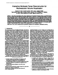
T according to Definition 2.3 are depicted Figure 2.1: General hyperbolic cross sets KK for D = 1 and N = 2. Here, wiso and wmix are given by (2.16) and (2.17), respectively.

The projection of a function f onto the general hyperbolic cross space VKT is given K T by with the help of the characteristic function χKT of the domain KK K

PKT [f ](~x) = F −1 [χKT fˆ](~x), K K DN Z 1 T~ = √ ei~x k fˆ(~k) d~k, T 2π KK

(2.21)

where we also write fKT := PKT [f ]. K

K

17

2 Sobolev Spaces for Many-Particle Functions t,r Lemma 2.1. Let t0 + r0 < t + r, t − t0 ≥ 0, f ∈ Hmix ((RD )N ) and fKT the projection of K f onto VKT . Then for t − t0 > 0 it holds K

kf − fKT kHt0 ,r0 K

mix

 −1 K (r0 −r)−(t−t0 )+(T (t−t0 )−(r0 −r)) NN−T kf kHt,r mix ≤ 0 −r)−(t−t0 ) (r K kf k t,r Hmix

for T ≥ for T ≤

r0 −r t−t0 , r0 −r t−t0 ,

(2.22)

and for t − t0 = 0 it holds kf − fKT kHt0 ,r0 K

mix

 −1 ) kf k t,r K (r0 −r)(1− NN−T Hmix ≤ 0 K (r −r) kf k t,r Hmix

for T > −∞, for T = −∞.

(2.23)

T in (RD )N by KT := (RD )N \ KT . Due to Proof. We denote the complement set of KK K K (2.21) the Fourier transform of fKT is given by χKT fˆ. Thus, we directly obtain K

kf − fKT k2 t0 ,r0 = K

Hmix

Z

K

(wmix (~k))2t (wiso (~k))2r |fˆ(~k)|22 dk 0

T KK

0

0 (wiso (~k))2(r −r) = (wmix (~k))2t (wiso (~k))2r |fˆ(~k)|2 d~k 0) 2(t−t ~ T (w ( k)) K mix K  Z 0 −r) 2(r ~ (wiso (k))   ≤ sup (wmix (~k))2t (wiso (~k))2r |fˆ(~k)|2 d~k 2(t−t0 ) ~ T (w ( k)) T K ~ mix k∈KK K   0 (wiso (~k))2(r −r)   = sup kf kHt,r . (2.24) mix ~ 2(t−t0 ) T (wmix (k)) ~

Z

k∈KK

T and Now, evaluating the supremum in (2.24) with the help of Definition 2.3 of the set KK 0 r0 −r −r with the help of either inclusion (2.19) with T1 = rt−t 0 , T2 = T for the case of T ≤ t−t0 0 −r r0 −r or inclusion (2.20) with T1 = T , T2 = rt−t 0 for the case of T ≥ t−t0 leads to the desired result for the case of t − t0 > 0 in (2.22). In the same way, estimate (2.23) for the case of t − t0 = 0 is obtained with the help of inclusion (2.19) for T = −∞ and inclusion (2.20) with T1 = T for T < −∞. 0

This type of estimate was already given for the case of measuring the error in the H0,r norm (i.e. t0 = 0) and a dyadically refined wavelet basis with D = 1 for the periodic case on a finite domain in [72, 73, 106, 107]. It is a generalization of the energy-norm based sparse grid approach of [23, 24, 64] where the case of t0 = 0, r0 = 1, t = 2, r = 0 was considered using a hierarchical piecewise linear basis. 0 Let us discuss some cases for measuring the error in the H0,r -norm (i.e. t0 = 0). For the 0,r standard Sobolev space Hmix (i.e. t = 0, 0 ≤ r0 < r) and the spaces VKT with T > −∞ K the resulting order is dependent on T and dependent on the number of particles N . In particular, the order even deteriorates with larger T . For the standard Sobolev spaces t,0 of bounded mixed derivatives Hmix (i.e. r = 0, 0 ≤ r0 < t) and the spaces VKT with K

18

2.3 Hyperbolic cross approximation 0

T > rt the resulting order is dependent on T and on the number of particles N whereas 0 for T ≤ rt the resulting order is independent of T and N . If for example we restrict the t,r 0,r class of functions to Hmix (i.e. t > 0, r ≥ 0) and measure the error in the Hmix -norm 0 (i.e. r = r), the approximation order is dependent on N for all T > 0 and independent on N and T for all T ≤ 0. Let us finally note that Lemma 2.1 can easily be extended to the case of employing wiso , wmix and ω given by (2.9), (2.10) and (2.11) in Definition 2.2 and 2.3. Figure 2.2 displays some example sets. 1/2

KK

−∞ KK

−2 KK

0 KK

−1/2

KK 5/6

−1/2

0 KK

0 KK 6/5

KK

15

10

10 5 5 0

0 −5

−5

−10 −10

−15 −10

−5

0

5

1 2

(a) The boundaries of the domains KK ⊂ −2 −∞ KK ⊂ KK for K = 10.

10 0 KK

−15 ⊂

−10

−5

0

5

10

15

−1/2

0 ⊂ (b) The boundaries of domains KK 5/6 ⊂ KK −1/2

KK

0 ⊂ KK 6/5 for K = 10.

T according to Definition 2.3 are depicted Figure 2.2: General hyperbolic cross sets KK for D = 1 and N = 2. Here, wiso and wmix are given by (2.9) and (2.10), respectively.

2.3.1 Multiscale decomposition of general hyperbolic cross spaces To obtain a multiscale decomposition of general hyperbolic cross spaces we use a Littlewood-Paley like dyadic partition of unity to decompose the Fourier space [57, 139]. To this end we consider the following index sets which are introduced in [72]: Definition 2.4. For T < 1 and L ∈ N we define the parametric index sets n o ILT := ~l ∈ NN : |~l|1 − T |~l|∞ ≤ L(1 − T ) + (N − 1) , with the natural extension to the case of T → −∞ by n o IL−∞ := ~l ∈ NN : |~l|∞ ≤ L .

19

2 Sobolev Spaces for Many-Particle Functions With regard to the cardinality of a set ILT , the following lemma is shown in [72, 73]: Lemma 2.2. It holds

X

2

|~l|1 −N

~l∈I T L

≤

 − 1/T1−1 −N L N  1 − 2 2 = O(2L )  2

for 0 < T < 1,

O(2    O(2LN )

for − ∞ < T < 0, for T = −∞.

−1 L TT /N −1

)

The case of T = 0 is covered by the additional estimate N −1 X ~ L |l|1 −N L N −2 2 ≤2 + O(L ) = O(2L LN −1 ), (N − 1)! T ~l∈I L

for 0 ≤ T ≤ 1/L. Now, for ILT according to Definition 2.4, we introduce a general hyperbolic cross [ KI T := Q~l, Q~l := Ql1 × · · · × QlN , (2.25) L

~l∈I T L

where we define the domain Ql ⊂ RD by o n Ql := k ∈ RD : 1 + (ω(k))2 ≤ 22l

(2.26)

for an index l ∈ N. Note that for l ∈ N the domain o n ˜ l := k ∈ RD : |k|∞ ≤ 2l Q

(2.27)

covers the Ql domain and thus it holds the inclusion [ ˜ T := ˜~, KI T ⊂ K Q I l L

L

~l∈I T L

˜~ := Q ˜l × · · · × Q ˜ l . Moreover, we have the following relation: with Q 1 N l T defined according to Definition 2.3 and K Lemma 2.3. Let T < 1, K ≥ 1, KK T as in IL (2.25) with L = dlog2 (K)e, then it holds the inclusion T KK ⊂ KI T . L

T . Then, by definition Proof. Let ~k ∈ KK   −T N Y 2 2  1 + (ω(kp ))  1 + max (ω(kp )) ≤ K 2(1−T ) . p=1

20

1≤p≤N

2.3 Hyperbolic cross approximation Now, for p = 1, . . . , N we set 1 2 lp := 1 + log2 1 + (ω(kp )) 2

and

∆lp := 1 +

1 log2 1 + (ω(kp ))2 − lp . 2

Then we have 1 + (ω(kp ))2 = 22(lp −1+∆lp ) , lp ∈ N, ∆lp ∈ [0, 1), and there follows the relation   −T N Y 2(l −1+∆l ) 2(l −1+∆l ) p p p p   max 2 2 ≤ 22 log2 (K)(1−T ) . 1≤p≤N

p=1

With pm = arg maxp=1,...,N (ω(kp ))2 we obtain  |~l|1 − T |~l|∞ ≤ log2 (K)(1 − T ) + (N − 1) − 

N X

 ∆lp + ∆lpm (1 − T )

p6=pm

≤ log2 (K)(1 − T ) + (N − T ) ≤ log2 (K)(1 − T ) + (N − 1) ≤ dlog2 (K)e(1 − T ) + (N − 1) = L(1 − T ) + (N − 1), which completes the proof. In order to obtain a multiscale decomposition of the general hyperbolic cross spaces VKT , we use a smooth dyadic decomposition of unity. To this end, for l ∈ N and Ql as K in (2.26) let ηQl : RD → [0, 1] an infinitely differentiable function such that ηQl (k) = 1 if k ∈ Ql , and supp ηQl ⊂ Ql+1 , i.e. a so-called bump function. Then we put η1 := ηQ1

and

ηl := ηQl − ηQl−1 , l ∈ {2, 3, 4, . . . }

(2.28)

and obtain with the help of the tensor product functions η~l := a partition of unity X ~l∈NN

N O

ηlp ,

~l ∈ NN ,

(2.29)

p=1

η~l(~k) = 1,

~k ∈ (RD )N .

(2.30)

Hence, every f ∈ S 0 splits into parts f~l(~x) := F −1 [η~lFf ](~x), i.e. it holds the relation

f (~x) =

X ~l∈NN

f~l(~x),

(2.31) (2.32)

21

2 Sobolev Spaces for Many-Particle Functions for f ∈ S 0 (with the usual distributive meaning), similar to a variant of Calderón representation formula in the case of inhomogeneous spaces [45, 57, 139]. Let us now consider the partial sum X fI T (~x) := f~l(~x), (2.33) L

~l∈I T L

which corresponds to a hyperbolic cross index set ILT of a multiscale decomposition (2.32) t,r of a function f ∈ Hmix . Here, the domain KI T covers the general hyperbolic cross K2TL L P due to Lemma 2.3 and by definition we have ~l∈I T η~l(~k) = 1 for ~k ∈ K2TL ⊂ KI T and L L P 0 ≤ ~ T η~(~k) ≤ 1 for ~k ∈ (RD )N \ KTL . Hence, f T approximates f at least as well l∈IL

l

IL

2

as the hyperbolic cross projection fKT given by (2.21), and analogously to Lemma 2.1 2L we obtain the following estimates: t,r Lemma 2.4. Let t0 + r0 < t + r, t − t0 ≥ 0, f ∈ Hmix ((RD )N ) and fI T ∈ VKI T as in L

(2.33). Then for t − t0 > 0 it holds  −1 ) kf k t,r 2L((r0 −r)−(t−t0 )+(T (t−t0 )−(r0 −r)) NN−T Hmix kf − fI T kHt0 ,r0 ≤ L 2L((r0 −r)−(t−t0 )) kf k t,r mix

for T ≥ for T ≤

Hmix

L

r0 −r t−t0 , r0 −r t−t0 ,

and for t − t0 = 0 it holds kf − fI T kHt0 ,r0 L

mix

 −1 ) kf k t,r 2L(r0 −r)(1− NN−T Hmix ≤ 2L(r0 −r) kf k t,r Hmix

for T > −∞, for T = −∞.

2.3.2 Approximation by general sparse grid spaces In the following we shortly discuss an approximation of the parts f~l as in (2.33), where t,r we assume that the function f is in Hmix ⊂ L2 , r + t ≥ 0, t ≥ 0 and that its Fourier ˆ t,ˆ r transform fˆ is in Hmix ⊂ L2 , rˆ + tˆ ≥ 0, tˆ ≥ 0. Let us remark, that as already discussed in Section 2.1.3 the regularity of the Fourier transform fˆ in the Fourier space is directly related to the decay of f for |~x|2 → ∞ in the spatial space. On this note, we introduce:

Definition 2.5. For t + r ≥ 0, t ≥ 0, tˆ + rˆ ≥ 0, tˆ ≥ 0 we define o n t,r;tˆ,ˆ r t,r tˆ,ˆ r Hmix := f ∈ Hmix : fˆ ∈ Hmix ⊂ L2 ⊂ L2 . Note that we may introduce an Hermitian inner product hf , giHt,r;tˆ,ˆr := hf , giHt,r + mix

mix

hfˆ , gîHtˆ,ˆr with the norm kf k2 t,r;tˆ,ˆr := hf , f iHt,r;tˆ,ˆr = kf k2Ht,r + kfˆk2 tˆ,ˆr . Now, let mix

Hmix

mix

mix

Hmix

%l ∈ C ∞ (RD ) for all l ∈ N be given such that %∗l %l = ηl with ηl according to (2.28) form a smooth partition of unity on RD . Then, corresponding to (2.29) we have with %~l :=

22

N O p=1

%lp ,

~l ∈ NN ,

2.3 Hyperbolic cross approximation the equivalence η~l = %~∗ %~l and hence {%~∗ %~l}~l∈NN form a smooth partition of unity on l l (RD )N as in (2.30). Thus, a term f~l given by (2.31) can be written as f~l = F −1 [%~∗l %~lfˆ] = F −1 [%~l gˆ~l],

(2.34)

where gˆ~l := %~∗ fˆ is at least as smooth as fˆ and of bounded support, i.e. supp gˆ~l ⊂ Q~l+~1 . l In particular, the support of fˆ T is covered by the domain IL

~

KI1 T := L

[

Q~l+~1 .

~l∈I T L

To obtain a finite-dimensional general sparse grid space each gˆ~l, ~l ∈ ILT may now be approximated by a spectral Galerkin method. To this end, let us suppose that we have an orthonormal basis {bj }j∈ZD for the space of square integrable functions on a a a 2 D D-dimensional torus TD a , Ta := [− 2 , + 2 ], a > 0, L (Ta ). Let us remark Sthat, except for the completion with respect to a chosen Sobolev norm, the union ∞ J=1 VJ with D J VJ := span{bj : j ∈ Z , |j|∞ ≤ 2 } is just the associated Sobolev space. Furthermore, we introduce the functions D 1 bl,j (k) := (al+1 )− 2 bj al+1 k (2.35) 1

with al := a2 (22l − 1) 2 , which form an orthonormal basis for L2 (Ql+1 ) and with it the functions b~l,~j (~k) :=

N O p=1

1

blp ,jp (~k) = | det A~l+~1 |− 2

N O p=1

bjp (A~−1~ ~k), l+1

~j ∈ (ZD )N ,

which then form an orthonormal basis for L2 (Q~l+~1 ), where the linear transformation A~l is given by N ~ (2.36) A~l : (TD a ) → Q~l : k 7→ (al1 k1 , . . . , alN kN ). We can then uniquely represent any gˆ~l as gˆ~l(~k) = with coefficients c~l,~j =

Z Q~l+~1

c~l,~j b~l,~j (~k)

X ~j∈(ZD )N

(2.37)

b~∗l,~j (~k)ˆ g~l(~k) d~k = hb~l,~j , gˆ~liL2

and we especially have kˆ g~lk2L2 ((RD )N ) = kˆ g~lk2L2 (Q

) ~ l+~ 1

=

P

~j∈(ZD )N

(2.38) |c~l,~j |2 = k{c~l,~j }~j k2`2 . Note

that the coefficients given in (2.38) may be also written with the help of the functions φ~l,~j := F −1 [%~l b~l,~j ] =

N O

φlp ,jp ,

φl,j (x) := F −1 [%l bl,j ](x)

(2.39)

p=1

23

2 Sobolev Spaces for Many-Particle Functions in the form c~l,~j =

Z Q~l+~1

(%~l (~k)b~l,~j (~k))∗ fˆ(~k) d~k = hφ~l,~j , f iL2 ((RD )N ) .

Inserting the series representation (2.37) in (2.34) results in X c~l,~j b~l,~j ]. f~l = F −1 [%~l

(2.40)

~j∈(ZD )N

See also [45, 57, 139]. Now, if we denote the partial sum of the series representation (2.40) associated with a finite subset JJR (~l) ⊂ (ZD )N by X f~l,J R (~l) := F −1 [%~l c~l,~j b~l,~j ] J

and introduce

~j∈J R (~l) J

fI T ,J R (~x) := L

J

X ~l∈I T L

f~l,J R (~l) ,

(2.41)

J

then it holds the relation kf − fI T ,J R kHt0 ,r0 = kf − fI T + fI T − fI T ,J R kHt0 ,r0 L

J

L

mix

L

L

J

(2.42)

mix

≤ kf − fI T kHt0 ,r0 + kfI T − fI T ,J R kHt0 ,r0 L

mix

L

L

J

mix

0

for t0 + r0 ≤ t + r, t − t0 ≥ 0. Furthermore, for either t0 = 0 or t0 > 0, rt0 ≥ T the estimate Z 0 0 kfI T − fI T ,J R k2 t0 ,r0 = (wmix (~k))2t (wiso (~k))2r |fÎ T (~k) − fÎ T ,J R (~k)|22 dk L L J L L J Hmix D N (R )   Z  2t0 2r0  ~ ~ |fÎ T (~k) − fÎ T ,J R (~k)|22 dk ≤  sup (wmix (k)) (wiso (k))  ~ I

K1 T

~ ~ k∈K1 T I

.2

L

2L(t0 +r0 )

L

L

kfÎ T − fÎ T ,J R k2L2 L

L

J

L

J

(2.43)

holds. In addition, kfÎ T − fÎ T ,J R kL2 = k L

L

J

X ~l∈I T L

(fˆ~l − fˆ~l,J R (~l) )kL2 ≤ J

X ~l∈I T L

kfˆ~l − fˆ~l,J R (~l) kL2 J

(2.44)

and for the approximation error with respect to the L2 -norm we obtain the estimate X X X kfˆ~l − fˆ~l,J R (~l) k2L2 = k%~l c~l,~j b~l,~j k2L2 ≤ k c~l,~j b~l,~j k2L2 = |c~l,~j |2 , (2.45) J

~j∈J R (~l) J

~j∈J R (~l) J

~j∈J R (~l) J

where JJR (~l) := (ZD )N \ JJR (~l). Now, let us assume that the system {bj }j∈ZD and the sequence of sets {JJR (~l)}J∈N are chosen such that each part f~l can be approximated by

24

2.3 Hyperbolic cross approximation appropriate partial sums f~l,J R (~l) up to arbitrary accuracy with respect to the L2 -norm J in the space V~l := span{φ~l,~j : ~j ∈ (ZD )N }, i.e. the sum on the right hand side of (2.45) can be made arbitrary small by an increase of the parameter J. Here, φ~l,~j is defined according to (2.39). Then, due to (2.44) and (2.43), the band-limited functions fI T can also arbitrarily well be approximated by appropriate L P t0 ,r0 partial sums fI T ,J R in the space VLT := ~l∈I T V~l with respect to the Hmix -norm. Hence, L J L both terms on the right hand side of (2.42) can be made arbitrarily small and thus a t,r;tˆ,ˆ r function f ∈ Hmix according to Definition 2.5 can also be approximated arbitrarily well t0 ,r0 by appropriate partial sums fI T ,J R with respect to the Hmix -norm. Note that such a L J T space VL can be associated with an infinitely extended general sparse grid. Let us remark here that it is easy to adapt the latter construction to the case of using a partition of unity {η~l}~l∈NN corresponding to (2.30) with η~l = %˜~∗ %~l where %˜~l, %~l ∈ C ∞ and also of using l biorthonormal Riesz basesP {˜bj }j∈ZD , {bj }j∈ZD instead of an orthonormal basis. P Especially, we would then have f~l = ~j∈J R (~l) c~l,~j F −1 [%~l b~l,~j ] and kf~l − f~l,J R (~l) k2L2 . ~j∈J R (~l) |c~l,~j |2 , J J J R where the coefficients are given by c~l,~j = (˜ %~l(~k)˜b~l,~j (~k))∗ fˆ(~k) d~k. For a further reading on using biorthonormal Riesz bases in particular with regard to stability of tensor product bases and norm equivalences for spaces built from intersections of tensor products of t,l Hilbert spaces, e.g. Hmix with l ≤ 0, spaces see also [72, 73]. In the following we discuss the use of an orthonormal Riesz basis in more detail, exemplified by an expansion of each gˆ~l in a Fourier series and using a smooth partition of unity with η~l = %~∗ %~l. l

Exemplary use of a Fourier series expansion To this end, we employ for the basis {bj }j∈ZD in (2.35) the Fourier basis e˜j , j ∈ ZD according to (2.18), which especially is an orthonormal basis of L2 (TD ), where TD = TD a, ˜ a = 2π. Moreover, for reasons of simplicity we set Q~l to Q~l from (2.27) and with it we set al := a2 2l for the linear transform in (2.36). In particular, the functions φ~l,~j in (2.39) can then be written in the form φ~l,~j (~x) =

N O p=1

φlp ,jp (~x) =

N O p=1

φlp (~x + A~−1~~j), l+1

D

φl := (al+1 2π)− 2 F −1 [%l ]

(2.46)

and for a certain resolution of unity {%~∗ %~l}~l∈NN correspond to an orthonormal tensor l product basis built from Meyer wavelets and Meyer scaling functions; see Appendix B.2. N ~ ∈ (ND Also, we assume that tˆ, rˆ ∈ N0 and that there exist Cm ~ > 0 for all m 0 ) , such that for all ~l ∈ NN the estimate ~ D N ~ ~ D~km %~l (~k) ≤ Cm ~ %~l (k) for all k ∈ (R ) ,

(2.47)

holds.

25

2 Sobolev Spaces for Many-Particle Functions Let u~l be a square integrable periodic function on Q~l+~1 , with the unique representation P tˆ,ˆ r -norm as in (2.12) the equivalence u~l(~k) = ~j∈(ZD )N u~l,~j b~l,~j (~k). Here, we have for the Hmix |||u~l|||2 tˆ,ˆr

Hmix (Q~l+~1 )

X

'

~j∈(ZD )N

ˆ

(wmix (A~−1~~j))2t (wiso (A~−1~~j))2ˆr |u~l,~j |2 , l+1

l+1

where terms are included on the right hand side which also depend on ~l. Now, let g˜ ˆ be tˆ,ˆ r D N the periodic extension of gˆ ∈ Hmix (Q~l+~1 ) onto (R ) . Then, it holds the relation X ˆ (wmix (A~−1~~j))2t (wiso (A~−1~~j))2ˆr |c~l,~j |2 ' |||g˜ˆ~l|||2 tˆ,ˆr = |||ˆ g~l|||2 tˆ,ˆr D N . l+1

~j∈J R (~l) J

l+1

Hmix (Q~l+~1 )

Furthermore, we define the subsets JJR (~l) ⊂ (ZD )N by [ I~ι+~l+~1 , Iα~ := Iα1 × · · · × IαN , JJR (~l) :=

Hmix ((R ) )

Iα := ZD ∩ Qα ,

(2.48)

~ι∈IJR

i.e. Iα ⊂ {k ∈ ZD : |k|∞ ≤ 2α }. This yields the relation 2

X ~j∈J R (~l) J

|c~l,~j | =

~j))−2ˆr X (wiso (A~−1 l+~1

(wmix (A~−1~~j))2tˆ ~j∈J R (~l) l+1 J 

ˆ

(wmix (A~−1~~j))2t (wiso (A~−1~~j))2ˆr |c~l,~j |2 l+1

(wiso (A~−1~~j))−2ˆr

l+1



ˆ l+1  (wmix (A~−1~~j))2t (wiso (A~−1~~j))2ˆr |c~l,~j |2 ˆ −1 l+ 1 l+1 2 t ~ R ~j∈J (~l) (wmix (A ~l+~1 j)) J ~j∈J R (~l) J

≤  max

'

max 2

−2tˆ|~ι|1 −2ˆ r|~ι|∞

X

!

~ι∈NN \IJR

|||ˆ g~l|||2 tˆ,ˆr

(2.49)

Hmix ((RD )N )

for the right hand side of (2.45). We summarize the discussion in a lemma. Lemma 2.5. Let r0 + t0 ≥ 0, t0 ≥ 0, t0 + r0 < t + r, t − t0 ≥ 0, rˆ, tˆ ∈ N0 , tˆ + rˆ > 0, t,r;tˆ,ˆ r f ∈ Hmix ((RD )N ), fI T as in (2.33) and fI T ,J R as in (2.41) (where bj , j ∈ ZD is set to L J L the Fourier basis e˜j , j ∈ ZD according to (2.18)). Additionally, let either t0 = 0 or t0 > 0, r0 ˆ t0 ≥ T . Then for t > 0 it holds that  N −1 2L(t0 +r0 ) 2−J(tˆ+ˆr−(Rtˆ+ˆr) N −R ) kfˆk tˆ,ˆr for R ≥ − rˆtˆ , Hmix kfI T − fI T ,J R kHt0 ,r0 . L L J 2L(t0 +r0 ) 2−J(tˆ+ˆr) kfˆk tˆ,ˆr mix for R ≤ − rˆtˆ , H mix

and for tˆ = 0 it holds that kfI T − fI T ,J R kHt0 ,r0 . L

26

L

J

mix

 N −1 2L(t0 +r0 ) 2−J rˆ(1− N −R ) kfˆk tˆ,ˆr H

for R > −∞,

2

for R = −∞.

L(t0 +r0 )

2−J rˆkfˆkHtˆ,ˆr

mix

mix

2.3 Hyperbolic cross approximation 3

3

3

2

2

2

1

1

1

0

0

0

−1

−1

−1

−2

−2

−2

−3 −3

−2

−1

0

1

2

3

−3 −3

−2

−1

0

1

2

3

−3 −3

5

5

5

4

4

4

3

3

3

2

2

2

1

1

1

0

0

0

−1

−1

−1

−2

−2

−2

−3

−3

−3

−4

−4

−4

−5 −5

−5 −5

−4

−3

−2

−1

0

1

2

3

4

5

15

15

10

10

5

5

0

0

−5

−5

−10

−10

−15

−4

−3

−2

−1

0

1

2

3

4

5

−5 −5

−2

−4

−1

−3

−2

0

−1

0

1

1

2

2

3

3

4

5

−15 −15

−10

−5

0

5

10

15

−15

−10

−5

0

5

10

15

0;0 Figure 2.3: Localization peaks of basis functions in VL;J according to (2.50) with D = 1 and N = 2. Here, we have L = 1, 2, 4 from left to right and J = 1, 2, 4 from top to bottom.

Proof. Evaluating the maximum in (2.49) leads to the desired result with (2.43), (2.44), (2.45) and (2.47). Here, the function fI T ,J R is in a finite-dimensional space L

T ;R VL;J

J

:= span(BV T ;R ), L;J

BV T ;R := {φ~l,~j : ~l ∈ ILT ,~j ∈ JJR (~l)}, L;J

(2.50)

which is a subspace of VLT and can be particularly associated with a general sparse grid.3 3

Let remark that, except for the completion with respect to a chosen Sobolev norm, the union S∞us S ∞ T ;R L=1 J=1 VL;J is just the associated Sobolev space.

27

2 Sobolev Spaces for Many-Particle Functions

T ;R according to (2.50) with D = 1 Figure 2.4: Localization peaks of basis functions in V4;4 1 and N = 2. Here, we have T = 2 , 0, −∞ from left to right and R = 21 , 0, −∞ from top to bottom.

T ;R Examples for the general sparse grid spaces VL;J in the case of the Meyer wavelet family with D = 1 and N = 2 are shown in Figure 2.3 and in Figure 2.4.4 Obviously, under the assumptions of Lemma 2.5, an upper bound estimate for the best approximation error t,r;tˆ,ˆ r t0 ,r0 of f ∈ Hmix in the Hmix -norm is given with

inf

T ;R f˜∈VL;J 4

kf − f˜kHt0 ,r0 ≤ kf − fI T ,J R kHt0 ,r0 mix

L

J

mix

(2.51)

Note that for the adaption to the case of the Meyer wavelet family given in B.2, we slightly modify the definition of index sets JJR (~l), where the approximation and complexity orders are not changed.

28

2.3 Hyperbolic cross approximation by equation (2.42) together with Lemma 2.4 and Lemma 2.5. Here, the aim is to choose the parameters such that the two error terms given in Lemma 2.4 and Lemma 2.5 are t,r;tˆ,ˆ r balanced. Let us shortly discuss the case of f ∈ Hmix with the assumptions of Lemma 0 −r rˆ 2.5 and T ≤ rt−t , R ≤ − . Then it holds the estimate 0 tˆ inf

T ;R f˜∈VL;J

J ˆ 0 0 0 0 kf − f˜kHt0 ,r0 . 2L((t +r )−(t+r)) kf kHt,r + 2L((t +r )− L (t+ˆr)) kfˆkHtˆ,ˆr mix

mix

mix

l m ˜ and for J(L) := L r+t in particular tˆ+ˆ r ˜ L(r + t) ≤ J(L)( tˆ + rˆ).

(2.52)

Thus, we obtain the relation 0 0 kf − f˜kHt0 ,r0 . 2L(t +r −(t+r)) kf kHt,r + kfˆkHtˆ,ˆr .

inf

f˜∈V T ;R ˜

mix

mix

L;J(L)

(2.53)

mix

In this case, the approximation rate according to Lemma 2.4 is preserved.5 T ;R The number of degrees of freedom, i.e. the dimension of VL;J , is equal to |BV T ;R | and L;J

thus to the cardinality number of the index set

n o T ;R IL;J := (~l,~j) : ~l ∈ ILT ,~j ∈ JLR (~l) ⊂ NN × (ZD )N . T ;(D)

Let us introduce the index set IL generalization of Lemma 2.2 by:

:=

S

~l∈I T L

(2.54)

I~l with I~l from (2.48), which leads to a

Lemma 2.6. For T < 1, L ∈ N it holds  DL  O(2 )   O(2DL LN −1 ) T ;(D) |IL |≤ −1 DL T T /N −1 )  O(2     O(2DLN )

for 0 < T < 1, for T = 0, for T < 0, for T = −∞.

(2.55)

Proof. Since it holds T ;(D)

|IL

5

|.

X ~l∈I T L

~

2D|l|1 . (

X

~

2|l|1 −N )D

~l∈I T L

We remark that for fˆ ∈ C ∞ the parameters rˆ and tˆ can be chosen arbitrarily high in dependence of J ˆ L such that the relation (t + r) ≤ L (t + rˆ) is fulfilled for a fixed J. However, the constants involved in the estimates are then also dependent on rˆ and tˆ.

29

2 Sobolev Spaces for Many-Particle Functions estimate (2.55) follows directly with Lemma 2.2 for all cases except for T = 0. The case of T = 0 results from X

2

D(|~l|1 −N )

=

L+N X−1

2D(j−N )

j=N

~l∈I 0 L

=

L−1 X

2

X

1

|~l|=j Dj

j=0

N −1+j N −1

L−1 X (N −1) 1 xj+N −1 = D (N − 1)! x=2 j=0 L (N −1) 1 N −1 1 − x x = D (N − 1)! 1−x x=2 (N −1−j) N −1 X 1 N −1 1 (j) = xN −1 − xL+N −1 (N − 1)! j 1−x j=0

x=2D

N −1 X L + N − 1 D(N −1−j) DL .2 2 j j=0

.2

DL N −1

L

.

See also [24, 73] and selected references therein. T ;R | can given with the help of Lemma 2.6 and the following An upper estimate for |IL;J lemma:

Lemma 2.7. For T < 1, L ∈ N, R < 1, J ∈ N it holds T ;(D)

T ;R | . |IL |IL;J

R;(D)

| |IJ

|.

(2.56)

Proof. We have |Iα~ | . 2D|~α|1 and thus with (2.54) and (2.48), relation (2.56) easily follows with X X ~ ~ T ;R |IL;J |. 2D|~ι+l+1|1 ~l∈I T ~ι∈JJR L

.

X ~l∈I T L

~

2D|l|1

X

2D|~ι|1 .

~ι∈IJR

All in all, according to estimate (2.53) and Lemma 2.7 the following result holds: For t,r;tˆ,ˆ r functions in Hmix with the assumptions of Lemma 2.5 the use of the generalized sparse 0 −r T ;R rˆ grid space VL; with T ≤ rt−t 0 , R ≤ − ˆ and (2.52) leads to a significant reduction ˜ t J(L)

30

2.3 Hyperbolic cross approximation −∞;R in the number of degrees of freedom compared to the full grid space VL; , while the ˜ J(L) approximation order is preserved. 0,r;tˆ,ˆ r Let us discuss some cases. For the spaces Hmix (i.e. t = t0 = 0, 0 ≤ r0 < r, tˆ+ rˆ > 0)

T ;R and the spaces VL; (i.e. R ≤ − rˆtˆ ) with T > −∞ the resulting approximation order ˜ J(L) with respect to L is dependent on T and dependent on the number of particles N . In particular the order even deteriorates with larger T , whereas for T = −∞ the order is independent on the number of particles N . However, since for T < 0 the dimension T ;(D) T ;R of IL with respect to L is exponentially dependent on N , the dimension of VL; ˜ J(L) with respect to L is also exponentially dependent on N . This reflects the curse of 0,r dimensionality which makes problems in isotropic Sobolev spaces Hmix intractable for ˆ

t,0;t,ˆ r higher values of N . For the spaces of bounded mixed derivatives Hmix (i.e. r = t0 = 0, 0 T ;R 0 ≤ r0 < t, tˆ + rˆ > 0) and the spaces VL; (i.e. R ≤ − rˆtˆ ) with T > rt the resulting ˜ J(L) approximation order is dependent on T and dependent on the number of particles N 0 whereas for T ≤ rt the resulting order is independent of T and N . Note that for T > 0 T ;(D)

the dimension of IL

0

with respect to L is independent of N . Thus, for T ∈ (0, rt ] R;(D)

T ;R the dependency of the dimension of VL; on N is given by the factor |IJ(L) | only. ˜ ˜ J(L)

t,r;tˆ,ˆ r For example if we restrict the class of functions to Hmix (i.e. t > 0, r ≥ 0, tˆ + rˆ > 0, rˆ r 0 R ≤ − tˆ ) and measure the error in the H -norm (i.e. t = 0, r0 = r), the approximation order with respect to L is dependent on N for all T > 0 and independent on N and T T ;(D) for all T ≤ 0. In that case, for T = 0, the dependence of the cardinality number |IL | on N is only logarithmic. This reflects the fact that it is here possible to get rid of the curse of dimensionality of the discretization of the standard isotropic Sobolev spaces at least to some extent. Note that in all cases the constants in the O-notation depend on N and D. We cast the estimates on the degrees of freedom and the associated error into a form which measures the error with respect to the involved degrees of freedom and reach the following lemma in a special case: t,r;tˆ,0 Lemma 2.8. Let t0 + r0 ≥ 0, t0 ≥ 0, t0 + r0 < t + r, t − t0 ≥ 0, tˆ ∈ N0 , tˆ > 0, f ∈ Hmix , 0 T ;R r −r t+r ˜ 0 = T ≤ t−t0 , R = 0 and J(L) = tˆ L. Then with M := |VL;J(L) | it holds ˜

inf

f˜∈V T ;R ˜

kf − f˜kHt0 ,r0 . mix

L;J(L)

Proof. For 0 = T ≤

r0 −r t−t0

M log2 (M )2(N −1)

− (t+r−(t0 +r0ˆ)) D(1+(t+r)/t)

kf kHt,r;tˆ,0 . mix

Lemma 2.7 yields the relation 0;0 M = |VL; | . 2DL(1+c) (cL2 )N −1 , ˜ J(L)

where c := (t + r)/tˆ. With the assumptions of the lemma the relation (2.53) holds.

31

2 Sobolev Spaces for Many-Particle Functions Therefore, the estimate 0 0 kf − f˜kHt0 ,r0 . 2L(t +r −(t+r)) kf kHt,r + kfˆkHtˆ

inf

f˜∈V 0;0˜

mix

mix

L;J(L)

2LD(1+c) L2(N −1)

.

! (t0 +r0 −(t+r)) D(1+c)

L2(N −1)

.

mix

M log2 (M )2(N −1)

(t0 +r0 −(t+r)) D(1+c)

kf kHt,r + kfˆkHtˆ mix

mix

kf kHt,r + kfˆkHtˆ

mix

mix

follows. Thus, the convergence rate is up to logarithmic terms independet of the number particles. Note however, that due to possibly large terms kf kHt,r , kfˆkHtˆ and the constants mix mix involved in the approximation and complexity order estimates, the generalized sparse grid discretization scheme is only practical for a moderate number of low-dimensional particles. This holds even if there are no exponentially or logarithmically dependent terms with respect to the discretization parameter L present.

2.4 Weighted many-particle spaces We discuss certain function spaces, i.e. so-called weighted spaces, which are related to a certain particle-wise decomposition of an N -particle function. Such a decomposition of an N -particle function f : (RD )N → C with respect to appropriate one-particle functions gp , p = 1, . . . , N reads as f (~x) =f∅

Y

gq (xq )

q∈N

X

+

f{p1 } (xp1 )

p1 ∈N

X

+

Y q∈N \{p1 }

f{p1 ,p2 } (xp1 , xp2 )

p1 N2 + MS ,

N 2

− MS electrons (3.11)

where MS ∈ {− N2 , . . . , −1, 0, 1, . . . , N2 } for even N and MS ∈ {− N2 , . . . , − 12 , 12 , . . . , N2 } (N,MS ) for odd N . In this way, the total spin projection MS~s is equal to MS . Therefore, in the following without loss of generality we only consider eigenvalue problems HΨ(N,MS ) = E (N,MS ) Ψ(N,MS ) , Ψ(N,MS ) (P ~x) = (−1)|P | Ψ(N,MS ) (P ~x),

∀P ∈ S (N,MS ) ,

(3.12)

which correspond to the N + 1 different class representative spin distributions ~s(N,MS ) according to (3.11). Here, we set S (N,MS ) := S~s(N,MS ) with |S (N,MS ) | = ( N2 + MS )!( N2 − MS )!. Note that the eigenfunctions Ψ(N,MS ) are spatial functions Ψ(N,MS ) : (R3 )N → R, where the spin coordinates ~s(N,MS ) impose the partial antisymmetry conditions. Hence, the spatial eigenfunctions Ψ(N,MS ) are in     N/2+MS N ^ ^ L2(N,MS ) :=  L2 (R3 ) ⊗  L2 (R3 ) , (3.13) p=1

p=N/2+MS +1

compare Section 2.5. In particular, the full wave function which is given by 1 X 1 1 Ψ : (R3 )N × {− , + }N → R : (~x, ~s) 7→ (−1)P Ψ(N,MS ) (P ~x)δP ~s,~s(N,MS ) , 2 2 N! P ∈SN

54

3.3 Variational formulation solves the full eigenvalue problem (3.9) [196]. Furthermore, we label the electrons which possess spin + 12 also by spin-up ↑ and label the electrons which possess spin − 21 by spin-down ↓. In this way, for an N -electron state function, we denote the number of spin-up particles by N↑ and the number of spin-down particles by N↓ . In particular it holds N = N↑ + N↓ with N↑ = MS +

N , 2

N↓ = MS −

N 2

(3.14)

for the total spin projection MS = 12 (N↑ − N↓ ). In the case of a spin-independent electronic Hamiltonian operator, it is sufficient to solve the bN/2c + 1 eigenvalue problems only, which correspond to spin vectors ~s(N,MS ) with a total spin projection of 0 ≤ MS ≤ N/2, i.e. 0 ≤ N↓ ≤ N↑ ≤ N . Since in this thesis we do not consider spin operators, we refer to textbooks on quantum chemistry like [85, 170]. However, let us note that besides the spin quantum number MS , there is another spin quantum number usually denoted by S. The exact eigenfunctions Ψ of a spin-independent electronic Hamilton operator H are also eigenfunctions of the total spin ˆ = MS Ψ and its squared-magnitude operator Sˆ2 Ψ = angular momentum operator SΨ S(S + 1)Ψ since Sˆ and Sˆ2 commute with H. For an N -electron state S and MS describe the total spin and its z component. In this framework states with S = 0, 12 , 1, 32 , . . . have multiplicity (2S + 1) = 1, 2, 3, 4, . . . and are denoted as singlets (1 Ψ), doublets (2 Ψ), triplets (3 Ψ), quartets (4 Ψ), . . . ; see [170]. Moreover, for the exact N -electron state the spin quantum number S equals 21 times the number of unpaired electrons, i.e. S = 12 |N↑ − N↓ |.

3.3 Variational formulation Note that the methods in this thesis used to compute an approximation of the solution of the electronic Schrödinger equation are based on the variational principle. Thus, we briefly resume the variational formulation of the eigenvalue problem (3.12). Here, due to the kinetic energy operator of the electrons we only consider wave functions in the Sobolev space H1 ((R3 )N ) ⊂ L2 ((R3 )N ). In the following for a shorter notation we write L2 and H1 instead of L2 ((R3 )N ) and H1 ((R3 )N ). Furthermore, we consider L2 -normed wave functions only, i.e. kΨkL2 = 1, which obey the partially antisymmetry conditions given 1 in (3.12). Now, let H(N,M ⊂ H1 denote the subspace of first-order weakly differentiable S) partially antisymmetric functions given by3 n o 1 1 |P | (N,MS ) ~ H(N,M := f ∈ H : (−1) f (P x ) − f (~ x ) = 0, ∀P ∈ S ⊂ L2(N,MS ) . S) 3

1 Note that H(N,M may also be introduced as the intersection space H1 ∩ L2(N,MS ) or may also be S) defined as the closure of n o S(N,MS ) := f ∈ S : (−1)|P | f (~x) − f (~x) = 0, ∀P ∈ S (N,MS )

in the space H1 .

55

3 Electronic Schrödinger Equation See also Definition (3.13) and Section 2.5. Let us further introduce the linear partial antisymmetrization projection operator A(N,MS ) : L2 ((R3 )N ) → L2(N,MS ) by A(N,MS ) f (~x) := AN↑ ⊗ AN↓ f (~x) X 1 = (−1)|P | f (P ~x), N↑ !N↓ ! (N,M ) P ∈S

(3.15)

S

where AN↑ and AN↓ denote the antisymmetric projections according to (2.79) for the subspaces L2 ((R3 )N↑ ) and L2 ((R3 )N↓ ), respectively. Here, L2(N,MS ) = A(N,MS ) (L2 ((R3 )N )) and the numbers N↑ and N↓ are determined by N and MS given in (3.14). 1 Now, a function Ψ(N,MS ) ∈ H(N,M with kΨ(N,MS ) kL2 = 1 is a weak solution of the S) eigenvalue equation (3.12) with the associated eigenvalue E (N,MS ) if hφ , HΨ(N,MS ) iL2 = E (N,MS ) hφ , Ψ(N,MS ) iL2

(3.16)

for all test functions φ in the Sobolev space H1 .4 It is sufficient to consider only test func1 tions φ(N,MS ) ∈ H(N,M , since the linear partial antisymmetrization projection operator S)

A(N,MS ) and the purely symmetric electronic Hamilton operator H commute [14]. Thus, 1 besides the identity A(N,MS ) φ(N,MS ) = φ(N,MS ) for φ(N,MS ) ∈ H(N,M , the identities S) hφ , HΨ(N,MS ) iL2 = hφ , HA(N,MS ) Ψ(N,MS ) iL2 = hA(N,MS ) φ , HΨ(N,MS ) iL2 , hφ , Ψ(N,MS ) iL2 = hφ , A(N,MS ) Ψ(N,MS ) iL2 = hA(N,MS ) φ , Ψ(N,MS ) iL2

(3.17)

hold. The smallest energy with respect to (N, MS ) is given by (N,MS )

Emin

=

min

1 Ψ∈H(N,M

S)

hΨ , HΨiL2 .

,kΨkL2 =1

(3.18)

Moreover, a normalized wave function which minimizes (3.18) corresponds to the lowest (N,M ) state with respect to (N, MS ) and we denote it by Ψmin S .5 Now let us assume that (N,M ) Emin S exhibits multiplicity one and let {Vκ }κ∈N be an arbitrary dense family of finite1 dimensional subspaces Vκ ⊂ H(N,M . Let further Eκ and Ψκ denote Galerkin approxiS) 1 mations associated with the lowest state in the finite-dimensional subspace Vκ ⊂ H(N,M , S) i.e. Eκ =

min

hΨ , HΨiL2 ,

Ψ∈Vκ ,kΨkL2 =1

Ψκ = argminΨ∈Vκ ,kΨkL2 =1 hΨ , HΨiL2 .

(3.19)

The bilinearform h· , H·iL2 can be extended to a bounded, symmetric and coercive bilinearform on H1 by a shift; see e.g. [192, 196]. (N,M ) (N,M ) 5 Note that the so-called ground-state ΨgroundS is associated with the minimal eigenvalue EgroundS := 4

(N,M )

min−N/2≤MS ≤N/2 Emin S . For a spin-independent electronic Hamiltonian operator it is usually given for MS = 0 in the case of even N and for MS = ±1/2 in the case of odd N .

56

3.4 Properties of the solution (N,M )

Then, Emin S ≤ Eκ for all κ ∈ N and thereby a relation between an estimate for the accuracy of an eigenfunction and an estimate for the approximation error of the lowest eigenvalue can be deduced, i.e. there exist C1 , C2 > 0 and κ ˜ ∈ N such that the relation (N,MS )

(N,MS )

(N,MS )

(N,MS )

− Ψκ k2H1 (3.20) holds for all κ ≥ κ ˜ ; see [161, 192]. For more details of the variational formulation of the eigenvalue problem (3.12) see also [192, 196]. 0 ≤ Emin

− Eκ ≤ C1 hΨmin

− Ψκ , H(Ψmin

− Ψκ )iL2 ≤ C2 kΨmin

3.4 Properties of the solution In the following we briefly review important properties of the solution of the N -electron Schrödinger equation (3.9).

3.4.1 Discrete spectrum and exponential bounds We consider the spectrum σ(H) of an electronic Hamilton operator H for molecules as in (3.3). In particular, the operator H is semibounded, self-adjoint and its discrete spectrum σdisc (H) is defined by the set of all isolated eigenvalues of finite multiplicity. Furthermore, the essential spectrum σess (H) is defined as the complement of the discrete spectrum σess (H) := σ(H) \ σdisc (H). Note further that in quantum mechanics the discrete spectrum corresponds to the so-called bound-states, whereas the so-called freestates correspond to the absolutely continuous spectrum. In this thesis we are only interested in the discrete spectrum and in particular in the ground-state energy E0 = inf σ(H). Let us add that in quantum mechanics the so-called exited-states correspond to the eigenfunctions with eigenvalues E ∈ σdisc (H) and E > E0 . The basis for all variational methods applied to the discrete spectrum constitutes the so-called HVZ (Hunziker, van Winter, and Zhislin) theorem [98]. From this theorem, it follows in the case of an N -electron electronic Hamilton operator H that the essential spectrum is given by σess (H) = [Σ, ∞), where the lower energy bound is equal to Σ = ˜ ≤ 0. Here, H ˜ denotes the electronic Hamilton operator which corresponds to inf σ(H) the fixed arrangement of nuclei associated with the electronic operator H but with one ˜ is an (N − 1)-electron Hamilton operator and thus Σ is electron less.6 In this way, H P nuc the so-called ionization threshold. In particular, if N ≤ N q=1 Zq holds for a system, e.g. in the case of atoms, molecules and positive ions, then the discrete spectrum is only below the essential spectrum, i.e. E0 ≤ E < Σ for all E ∈ σdisc (H), and the discrete spectrum consists of infinitely many eigenvalues [98, 163]. On the other hand P nuc it is known that in the case of N ≥ Nnuc + 2 N Z the discrete spectrum is empty q q=1 [124]. Furthermore, eigenfunctions which are associated with eigenvalues of the electronic Hamilton operator in the discrete spectrum are known to decay exponentially [2]. In particular, the exponential decay of a wave function Ψ is described by an L2 exponential 6

Note that the lowest energy of a system with N = 0 is equal to zero.

57

3 Electronic Schrödinger Equation bound, i.e. there is a positive function h with Z eh(~x) |Ψ(~x)|2 d~x < ∞. (R3 )N

(3.21)

Note that in general, an in some sense optimal bound should be anisotropic [2, 98]. To this end, Agmon expressed in his seminal work [2] an anisotropic bounded function h as a geodesic distance in terms of a certain Riemannian metric which takes different ionization thresholds into account. With the help of this so-called Agmon distance the anisotropic exponential decay of the eigenfunctions associated with eigenvalues in the discrete spectrum can be described accurately. As an example from [2], we recall the case of an atom within the Born-Oppenheimer approximation. Here, Agmon studies in detail the L2 -decay of the eigenfunctions of the electronic Hamiltonian H of an atom with one nucleus fixed in the origin of the coordinate system. To this end, for I ⊂ {1, . . . , N } let HI denote the restriction of the full Hamiltonian H to the subsystem involving only the electrons associated with I and ΛI = inf σ(HI ), ΛI = 0 if I is empty. For any ~x ∈ (RD )N \ {~0} let I(~x) denote the subset of integers p ∈ {1, . . . , N } for which xp = 0. Now, for eigenfunctions Ψ with an eigenvalue E in the discrete spectrum of H, a characterization of the type (3.21) with a positive function haniso : (R3 )N → R : ~x 7→ 2(1 − ε)ρ(~x) for any ε > 0 is given in [2]. Here, ρ(~x) is the geodesic distance from ~x to the origin in the Riemannian metric N X 2 d~s = (ΛI(~x) − E) 2|dxp |22 . i=1

Note that ρ is not isotropic. It takes into account the amount of electrons with position 0, i.e. the number of electron-nucleus cusps, at each point ~x. 1 However, there are also useful isotropic bounds. For example, if Ψ(N,MS ) ∈ H(N,M S) is a weak solution of the eigenvalue problem (3.12) with the electronic Hamiltonian for molecules (3.3), and if the associated eigenvalue is below the ionization threshold Σ(N,MS ) , i.e. E (N,MS ) < Σ(N,MS ) , then Ψ(N,MS ) and ∇Ψ(N,MS ) decay exponentially in the L2 -sense, i.e. Z Z ehiso (~x) |Ψ(N,MS ) (~x)|2 d~x < ∞ and ehiso (~x) |∇Ψ(N,MS ) (~x)|22 d~x < ∞ (R3 )N

(R3 )N

with 3 N

hiso : (R )

q → R : ~x 7→ 2(Σ0 − E (N,MS ) )|~x|2

for E (N,MS ) < Σ0 < Σ(N,MS ) ; see [196] and selected references therein. For more details on the general basics of Schrödinger operators and the quantum N -body problem see the review articles [98, 163]. In particular, with respect to Coulomb systems see [125] and concerning the anisotropic exponential decay of the bound-states see [2].

58

3.4 Properties of the solution

3.4.2 Cusp conditions and regularity results At first, let us consider the eigenvalue problem HΨsl = E sl Ψsl

(3.22)

with the spin-independent electronic Hamilton operator (3.3) and without any side conditions due to spin. Note that the spatial electronic wave functions Ψ(N,MS ) according to the eigenvalue problem (3.12) also solve the eigenvalue problem (3.22). Since in the case of D = 3 the Coulomb potential |x|1 2 is only unbounded at x = 0, the interaction potentials Vne and Vnn are only singular at the set of coalescence points      N Y N N N nuc   Y Y Y |xp − Rq |2   (3.23) |xp − xp0 |2  = 0 . C := ~x ∈ (R3 )N :    0 p=1 q=1

p=1 p >p

Thus, the spinless eigenfunctions Ψsl : (R3 )N → R are nonanalytic on C and analytic elsewhere (R3 )N \ C. In 1957, Kato proved that the spinless N -electron wave functions Ψsl are locally Lipschitz [104]. Moreover, in [104] he analyzed the behaviour of spinless N -electron wave functions Ψsl of an atom near coalescence points ~rC ∈ C with exactly one singular term in the interaction potential Vne + Vnn , the so-called two-particle coalescence points. By assuming that Ψsl does not vanish at the coalescence point ~rC ∈ C, i.e. Ψsl (~rC ) 6= 0, he proved the so-called cusp conditions, i.e. conditions an eigenfunction has to obey at a coalescence point ~rC ∈ C. For example, Kato’s cusp conditions in the case of an N electron atom of charge Z centered at the origin for coalescence points ~rC ∈ C and an electron-nucleus cusp with rCp = 0 (w.l.o.g. let p = 1) reads as ˜ sl ∂Ψ = −ZΨsl 0, rC2 , . . . , rCN , (3.24) ∂r1 r1 =0

˜ sl denotes the spherical average of Ψsl over an infinitesimally small where r1 = |r1 |2 and Ψ C sphere at r1 = 0. Concerning an electron-electron cusp for ~rCi −~rCj = 0 (w.l.o.g. let i = 1 and j = 2) the cusp condition can be written in the form ˜ sl ˜ ∂Ψ = 12 Ψsl 12 (r1 + r2 ), 12 (r1 + r2 ), rC3 , . . . , rCN , (3.25) ∂r12 r12 =0

˜ ˜ sl denotes the spherical average of Ψsl over an infiniteswhere r12 = |r1 − r2 |2 and Ψ 1 imal small sphere about 2 (r1 + r2 ) with constant r12 . Note that due to the partially antisymmetry conditions (3.12), the spatial part of an N -electron wave function Ψ(N,MS ) vanishes at a coalescence point of more than two electrons. Thus, besides the case of molecules and the case of coalescence points of more than two particles, Kato’s cusp

59

3 Electronic Schrödinger Equation conditions have been particularly generalized to the case of an eigenfunction Ψsl which vanishes at the considered coalescence point Ψsl (~rC ) = 0. This has been done by several authors, e.g. by Pack et al. [149], Hoffmann-Ostenhof et al. [94, 95] and Tew [174]. Let us recall now some of their main results. In [149] for two-particle cusp conditions Pack et al. derive an extension to Kato’s results by analysing an expansion in terms of real spherical harmonics of a spinless eigenfunction of (3.22) in the vicinity of any two particles’ coalescence. Especially, the case of an N -electron wave function Ψsl , which may vanish at the considered two-particle coalescence point ~rC , is also included. In the case of Ψsl (~rC ) 6= 0 for a given two-particle electron-electron coalescence point ~rC ∈ C the cusp condition 2 Ψsl r1 , r2 , rC3 , . . . , rCN = Ψsl 21 (r1 + r2 ), 12 (r1 + r2 ), rC3 , . . . , rCN 1 + 12 r12 + O r12 (3.26) holds, and in the case that Ψsl vanishes by first order in ~rC , there follows the cusp condition sl 3 Ψsl r1 , r2 , rC3 , . . . , rCN = ~rT12 ∂Ψ 1 + 41 r12 + O r12 . (3.27) ∂~r12 r12 =0

Note that the electron-electron cusp condition (3.26) is valid for the singlet state helium, i.e. the state which possesses minimal energy for two electrons of opposite spin, and the electron-electron cusp condition (3.26) is valid for the triplet state of helium, i.e. the state which possesses minimal energy for two electrons of same spin. In [157] for the first order derivatives of a spherically averaged wave function, Kato’s cusp conditions (3.24) and (3.25) were extended to the case of the third order derivatives of a spherically averaged wave function. More recently, the results of Pack et al. were improved by Tew [174]. Here, the structure of the wave function is examined to second and higher orders in vicinity of the coalescence of any two charged particles, if these are well separated from all other particles. The case of many-particle coalescence and the influence of partially antisymmetry due to spin is considered by Hoffmann-Ostenhof et al. in [94, 95]. In these works the authors show that for any given coalescence point ~rC ∈ C, there exists a harmonic homogeneous polynomial PMP 6= 0 of degree MP , i.e. ∆PMP = 0 and PMP (λ~r) = λMP PMP (~r) for λ ∈ R, which describes the behaviour of a spinless N -electron wave function Ψsl for |~r − ~rC |2 → 0. Then the cusp condition P +1 Ψsl (~r) = PMP ~r − ~rC + O |~r − ~rC |M (3.28) 2 holds near the coalescence point ~rC , and PMP can be written as 1 P PMP (~r) = |~r|M r , 2 YMP |~r|2 ~ where YM P denotes a multi-dimensional hyperspherical harmonic. In addition, HoffmannOstenhof et al. consider the minimal order of zeroes in a coalescence point in the case of a spatial N -electron wave function Ψ(N,MS ) with partial antisymmetry conditions according to (3.12). Note that the symmetry conditions on the wave function in (3.28)

60

3.4 Properties of the solution carry over to PMP . Hence, the minimal vanishing order of Ψ(N,MS ) in a given coalescence point ~rC ∈ C is equal to the minimal degree of PMP in (3.28) such that PMP satisfies the partial antisymmetry conditions according to (3.12) and PMP 6≡ 0. Therefore, HoffmannOstenhof et al. give the minimal degree of PMP in dependence of the number of electrons N and the total spin projection MS . In addition, they show that the minimal degree 4 increases for large N like O(N 3 ). Furthermore, a theorem about the regularity of the spinless N -electron wave functions was recently shown by Fournais et al. in [55]: Theorem 3.1 (Fournais et al. [55]). Let Ψsl : (R3 )N → R : ~x 7→ Ψsl (~x) be an eigenfunction according to the spinless eigenvalue problem (3.22) and let F(en,ee,een) : (R3 )N → R : ~x 7→ F(en) (~x) + F(ee) (~x) + F(een) (~x) with the electron-nuclei correlation term F(en) (~x) :=

N X

f(en) (xp ),

f(en) (x) := −

N nuc X

p=1

Zq |x − Rk |2 ,

q=1

the electron-electron correlation term F(ee) (~x) :=

N X N X

f(ee) (xp , xp0 ),

p=1 p0 >p

1 f(ee) (x, y) := |x − y|2 2

and the electron-electron-nuclei correlation term F(een) (~x) :=

N X N X

f(een) (xp , xp0 ),

p=1 p0 >p

f(een) (~x) :=

Nnuc 2−π X (x − Rq )T (y − Rq ) ln |x − Rq |22 + |y − Rq |22 . 6π q=1

Then the eigenfunction Ψsl can be expressed in the form Ψsl = eF(en,ee,een) Φsl (en,ee,een) with a function

3 N Φsl x 7→ Φsl x) (en,ee,een) : (R ) → R : ~ (en,ee,een) (~

in the Hölder space C 1,1 ((R3 )N ).7 This representation is optimal in the following sense: There is no other function F ~ and Z ~ only, but not on Ψsl or E sl , such that Ψsl = F Φsl which is dependent on N , R sl with a function Φ having more regularity than C 1,1 . 7

The definition of the Hölder spaces C m,α with m ∈ N0 , α ∈ [0, 1] is recalled in Appendix A.1.

61

3 Electronic Schrödinger Equation Note that expressing a wave function as a product Ψ = F Φ is common in computational quantum physics and quantum chemistry, where F is a so-called Jastrow factor. Especially, in the case of an N -electron wave function F is usually assumed to be symmetric with respect to the permutation of particles and Φ is assumed to be antisymmetric (or partially antisymmetric) due to Pauli’s principle. Note further that the ansatz sl 1,α for α ∈ (0, 1), leads to a more general Ψsl = eF(en) +F(ee) Φsl (en,ee) , where Φ(en,ee) ∈ C formulation of Kato’s cusp conditions ∇Ψsl − Ψsl (∇F(en) + ∇F(ee) ) ∈ C 0,α for 0 < α < 1. Moreover, by including electron-electron-nuclei coalescence by the function F(een) Theorem 3.1 results in ∇Ψsl − Ψsl (∇F(en) + ∇F(ee) + ∇F(een) ) ∈ C 0,1 ,

(3.29)

which can be viewed as a cusp condition for second order derivatives [55]. Additionally, in [55], with respect to the regularity of the wave function near the zero-set o n N (Ψsl ) := ~x ∈ (R3 )N : Ψsl (~x) = 0 , Theorem 3.1 implies that ∇Ψsl : N (Ψsl ) 7→ (R3 )N is locally Lipschitz in contrast to Ψsl , which is just locally L∞ in C \ N (Ψsl ). Further results on the regularity of the eigenfunctions of the Schrödinger operator and on the behavior of a many-electron wave function in the neighborhood of the coalescence points can also be found in [54, 56]. Recently, in [52] Flad et al. discuss the application of the best M -term approximation theory [41] within the framework of a Jastrow-type ansatz for a wave function Ψ = F Φ, where the symmetric Jastrow factor J is assumed to be given in exponential form J = eF(1,...,N ) with a decomposition of the symmetric function F(1,...,N ) into manyelectron correlation functions.8 This decomposition is a special case of the particle-wise decompositions introduced in Section 2.4 and reads as F(1,...,N ) (~x) =

N X p=1

f(1) (xp ) +

N X N X p=1

f(2) (xp , xp0 ) + · · · + f(N ) (x1 , . . . , xN ).

p0 >p

In [52] the Besov regularity, which is related to the optimal convergence rate of best M -term approximations [41], of two-electron correlation functions f(2) : (R3 )2 → R : (x, y) 7→ f(2) (x, y) is analyzed for certain natural assumptions on the asymptotic behaviour of f(2) near electron-electron and electron-nucleus cusps. Note that the two-electron correlation functions f(2) typically provide the dominant contribution to the Jastrow factor J since oneelectron contributions to the wave function Ψ are usually included within the antisymmetric (or partially antisymmetric) factor Φ and since contributions to the Jastrow factor 8

A Jastrow factor in exponential form J = eF(1,...,N ) is commonly used in quantum mechanics since then J provides the so-called cluster property, and the so-called size-consistency is guaranteed for extended systems; see [52] and selected references therein.

62

3.4 Properties of the solution J according to three-electron and higher order terms f(n≥3) can normally be assumed to be negligibly small. In particular, Flad et al. consider the best M -term approximation spaces Aαq (H1 ) due to Nitsche [146] for certain anisotropic tensor product wavelet bases to prove that f(2) ∈ Aαq (H1 ) for q > 1 and α = 1q − 12 . In this way, they deduce that there exists an upper bound for the approximation error in the H1 -norm with respect to the number M of basis functions in the framework of the best M -term approximation of two-electron correlation functions. Here, an upper bound is given by   M 

 X 1

M M = cj φµj . M − 2 + , inf f(2) − f(2)

1 : f(2)   H

∀ > 0,

j=1

where {φµ : µ ∈ N0 } is a given anisotropic wavelet basis of certain type which possesses a number of vanishing moments equal to or greater than three.

3.4.3 Decay of weak mixed derivatives This thesis is basically motivated by the regularity results of Yserentant with respect to the eigenfunctions of the electronic Hamilton operator. Thus, we recall his mayor results from [193, 195, 196]. Let us first consider an arbitrary eigenfunction of the electronic Hamilton operator which obeys Pauli’s principle. 1 Theorem 3.2 (Yserentant [193]). Let Ψ(N,MS ) ∈ H(N,M a weak solution of the elecS) 1

,1

1,1 2 tronic Schrödinger equation (3.16). Then Ψ(N,MS ) is in Hmix and even in Hmix for an N N electronic wave function of totally parallel spin, i.e. MS ∈ {+ 2 , − 2 }.

To be precise, Yserentant shows in [193] that an eigenfunction Ψ(N,MS ) associated with a spin distribution ~s(N,MS ) has certain square integrable mixed derivatives of order up to N↑ + 1 Z ˆ (N,MS ) (~k)|2 d~k < ∞ (wmix, 1 (~k))2 (wiso (~k))2 |Ψ (R3 )N

2

with respect to the spatial coordinates x1 , . . . , xN↑ and certain square integrable mixed derivatives of order up to N↓ + 1 Z (R3 )N

ˆ (N,MS ) (~k)|2 d~k < ∞ (wmix,− 1 (~k))2 (wiso (~k))2 |Ψ 2

63

3 Electronic Schrödinger Equation with respect to the spatial coordinates xN↑ +1 , . . . , xN .9 Here, wmix,s is given by q  QN↑ (1 + (ω(k ))2 ) p ~ wmix,s (k) := qQp=1 N  2 p=N↑ +1 (1 + (ω(kp )) )

for s = + 21 ,

(3.30)

for s = − 21

1,1 Hence, a fully antisymmetric solution, i.e. MS ∈ {+ N2 , − N2 }, possesses Hmix -regularity. N Furthermore, in the case of an arbitrarily chosen total spin projection − 2 ≤ MS ≤ N2 , the inequality

Z (R3 )N

ˆ (N,MS ) (~k)|2 d~k wmix (~k)(wiso (~k))2 |Ψ Z 1 X ˆ (N,MS ) (~k)|2 d~k (wmix,s (~k))2 (wiso (~k))2 |Ψ ≤ 2 3 N (R ) 1 1 s∈{− 2 , 2 }

holds due to the elementary relation N Y j=1

N↑ 1Y 1 |˜ ω (kj )| ≤ |˜ ω (kj )|2 + 2 2 j=1

for 0 ≤ N↑ ≤ N with ω ˜ : R3 → R : k 7→ 1

N Y

|˜ ω (kj )|2

j=N↑ +1

p 1 + |ω(k)|2 . Thus, any partially antisymmetric

,1

2 wave function possesses at least Hmix -regularity. In the following we consider the approximation error with respect to general hyperbolic cross spaces VKT . Here, with D = 3, t0 = 0 and r = 1, according to Theorem 3.2 and K Lemma 2.1, the estimate

kΨ(N,MS ) − PKT [Ψ(N,MS ) ]kHr0 K  −1 K (r0 −1)−t+(T t−(r0 −1)) NN−T kΨ(N,MS ) kHt,1 mix ≤ K (r0 −1)−t kΨ(N,MS ) k t,1 Hmix

for T ≥ for T ≤

r0 −1 t , 0 r −1 t

(3.31)

holds for r0 < t + 1 with t = 1 in the fully antisymmetric case and t = 21 in case of an arbitrary total spin projection MS . Especially, let us discuss the case of a fully antisymmetric solution and the resulting approximation rate with respect to general hyperbolic cross spaces VKT in more detail. If we measure the approximation error K in the H1 -norm, then from Lemma 2.1 we obtain with t0 = 0, r0 = 1 and t = r = 9

Here, Yserentant uses wiso (~k) =

q

1+

PN

2 p=1 (ω(kp )) ,

8q < 1 + QN↑ (ω(kp ))2 p=1 wmix,s (~k) = q 2 : 1 + QN p=N↑ +1 (ω(kp ))

for s = + 12 , for s = − 12 .

and ω(k) = |k|2 which is (up to constants) equivalent to our definitions in (2.16), (3.30) and (2.15).

64

3.4 Properties of the solution 1 the approximation order O(K −1+T ( N −T ) ) for T ≥ 0 and O(K −1 ) for T ≤ 0. In particular, for the choice T = 0 a rate of O(K −1 ) results. In an analogous way we can argue for the partially antisymmetric case. Then, for an arbitrarily chosen total spin 1/2,1 projection − N2 ≤ MS ≤ N2 we have Hmix -regularity at least for the associated wave function. If we measure the approximation error in the H1 -norm, the approximation N −1 1 order O(K −1+T N −T ) for T ≥ 0 and O(K − 2 ) for T ≤ 0 is obtained from Lemma 2.1 N −1

1

,1

2 with t0 = 0, r0 = 1 and t = 12 , r = 1 (Hmix -regularity). In this case, let us consider the employment of the general sparse grid discretization scheme introduced in Section 2.3.2. ˆ (N,MS ) ∈ Htˆ,0 , tˆ > 0. Then, with the help of To this end, we additionally assume that Ψ mix Lemma 2.8, we obtain − 1 6(1+c) M (N,MS ) ˜ − ΨkH1 . inf kΨ kΨ(N,MS ) k 12 ,1;tˆ,0 , 2(N −1) 0;0 ˜ log (M ) Hmix Ψ∈V 2 ˜ L;J(L)

0;0 where c = 3/(2tˆ) and M = |VL; | denotes the number of the involved degrees of ˜ J(L) ˆ (N,MS ) is smooth, i.e. if Ψ(N,MS ) freedom. Here, we have c → 0 if the Fourier transform Ψ decays sufficiently fast (cf. Section 2.1.3). In particular, up to logarithmic terms, the convergence rate is independent of the number of electrons N and almost the same as in 1 the two-electron case. Thus, we obtain a rate of order − 6(1+c) and hence due to (3.20) 2 a rate of order − 6(1+c) for the minimal eigenvalue. t,r However, the constants involved in a norm equivalence on Hmix may depend on N and 1

,1

1,1 2 -terms may grow exponentially with the D. Moreover, in (3.31) also the Hmix - and Hmix number N of electrons. This is a serious problem for any further discretization of the general hyperbolic cross spaces VKT . In order to compensate for this exponential growth, K the parameter K has to be chosen dependent on N . Such a behavior can be observed in the case of a finite domain with periodic boundary conditions with Fourier bases from the results of the numerical experiments in [69] and was one reason why problems with higher numbers of electrons could not be treated. Recently, in [195] Yserentant suggested a rescaling of the mixed Sobolev norm and the 1,r general hyperbolic cross space. To this end, a scaled analog of the Hmix -norm, r ∈ {0, 1}, 1 1 is introduced for s ∈ {− 2 , + 2 } with a scaling parameter Θ via !!2  N r Z 2 X ~k kj ˆ (N,MS ) (~k)|2 d~k,   |Ψ kΨ(N,MS ) k2H1,r = wmix,s ω Θ Θ D N mix,Θ,s (R ) j=1

where wmix,s and ω are set corresponding to (3.30) and (2.11).  !!2  ~k (N,MS ) D N KK,Θ := ~k ∈ (R ) : wmix,− 1 + wmix, 1 2 2  Θ

(3.32) Furthermore, the domain  !!2  ~k 2 ≤K (3.33)  Θ

in Fourier space describes a Cartesian product of two scaled regular hyperbolic crosses. In the extreme case of totally parallel spin, i.e. MS ∈ {+ N2 , − N2 }, it degenerates into just

65

3 Electronic Schrödinger Equation

(2,0)

(2,0)

KΘK,1

(2,0)

K2K,Θ

(2,0)

(2,1)

K2KΘ,1

5

5

4

4

3 2 1 0

(2,1)

KK,Θ

log(1 + k2 )

log(1 + k2 )

KK,Θ

KΘ2 K,1

(2,1)

K2K,Θ

(2,1)

K2KΘ2 ,1

3 2 1

0

1

2 3 log(1 + k1 )

4

0

5 (2,0)

0

1

2 3 log(1 + k1 )

4

5 (2,1)

(a) The boundaries of the domains KK,Θ ⊂

(b) The boundaries of the domains KK,Θ ⊂

KKΘ2 ,1 , K2K,Θ ⊂ K2KΘ,1 for K = 8, Θ = 2 .

KKΘ2 ,1 , K2K,Θ ⊂ K2KΘ2 ,1 for K = 8, Θ = 2 2 .

(2,0)

(2,0)

3 2

(2,0)

(3, 3 )

(3, 3 )

KK,Θ2

2 KΘ3 K,1

8

(3, 3 )

(3, 3 )

2 K2K,Θ

2 KΘ3 K,1

8

(3, 3 )

(3, 3 )

2 K2K,Θ

2 K2KΘ 3 ,1

6 log(1 + k2 )

log(1 + k2 )

(3, 3 )

KK,Θ2

4

2

4

2

0

2

4 log(1 + k1 )

6 (3, 3 )

3) (3, 2 K2K,Θ

KKΘ3 ,1 , and k3 = 0.

3) (3, 2

0

8

(c) The boundaries of the domains KK,Θ2 (3, 3 ) 2

3

(2,1)

(3, 3 )

2 K2KΘ 3 ,1

6

0

(2,1)

(2,1)

⊂

⊂ K2KΘ3 ,1 for K = 8, Θ = 3

3 2

0

2

4 log(1 + k1 )

6

8 (3, 3 )

(d) The boundaries of the domains KK,Θ2 3) (3, 2

3) ) (3, 2 (3, 3 2 KKΘ3 ,1 , K2K,Θ ⊂ K2KΘ 3 ,1 and k3 = 21 (k1 + k2 ).

⊂ 3

for K = 8, Θ = 3 2

Figure 3.1: The case D = 1 scaled (Θ > 1) and non-scaled (Θ = 1): Hyperbolic cross (N,M )

sets KK,Θ S according to (3.33) are depicted for two particles which possess opposite spin (a), for two particles which possess parallel spin (b) and for three particles which possess totally parallel spin (c)-(d).

66

3.4 Properties of the solution one scaled regular hyperbolic cross. For examples of the case of two and three particles with D = 1 see Figure 3.1. The projection of a function f onto the scaled hyperbolic (N,M ) cross space VK,Θ S , i.e. the space of functions with vanishing Fourier transforms outside (N,MS )

the domain KK,Θ P

, is given by

(N,MS )

KK,Θ

[f ](~x) = =

1 √ 2π

3N Z

1 √ 2π

3N Z

(RD )N

ei~x

(N,MS

KK,Θ

T~ k

ei~x )

(N,M )

χ

(N,MS )

KK,Θ

T~ k

(~k)fˆ(~k) d~k

fˆ(~k) d~k (N,M )

with the help of the characteristic function χK,Θ S on the domain KK,Θ S . Then, in the case of D = 3 with the projection P (N,MS ) , the following error estimate is shown in [195]:

KK,Θ

1 Theorem 3.3 (Yserentant [195]). Let Ψ(N,MS ) ∈ H(N,M be an eigenfunction of the S) electronic Schrödinger equation according to (3.16) which possesses a negative eigenvalue E < 0. Then there exists a scaling parameter Θ such that the estimates of the approximation error measured in the L2 -norm √ 2 e (N,MS ) (N,MS ) (N,MS ) (3.34) kΨ kL2 kΨ − P (N,MS ) [Ψ ]kL2 ≤ KK,Θ K

and of the approximation error measured in the H1 -seminorm √ 2 e (N,MS ) (N,MS ) |Ψ − P (N,MS ) [Ψ ]|H1 ≤ ΘkΨ(N,MS ) kL2 KK,Θ K

(3.35)

hold.

√ In particular, there is a minimal scaling parameter Θ . N max(N, Z) such that the estimates (3.34) and (3.35) hold for all admissible eigenfunctions of corresponding PNnuc symmetry for negative eigenvalues [195], where Z = q=1 Zq is total charge of the nuclei. Especially, for an electronically neutral system we obtain Z = N and thus Θ . N 3/2 . The scaling parameter Θ relates to the intrinsic length scale of the atom or molecule under consideration; see [151, 195]. Let us note that the restriction to eigenfunctions of the electronic Schrödinger Hamiltonian whose associated eigenvalues are strictly smaller than zero is not a severe issue since such an assumption holds for bound-states, i.e. states in the discrete spectrum. Also, compare Section 3.4.1 and [98, 163]. This surprising result shows that, with proper scaling in the norms and the associated (N,M ) choice of a scaled hyperbolic cross, it is possible to get rid of the kΨK,Θ S kH1,l -terms mix on the right hand side of hyperbolic cross estimates of the type (3.31). Note that these (N,M ) terms may grow exponentially with N whereas kΨK,Θ S kL2 = 1. To derive semidiscrete approximation spaces which, e.g. after scaling, overcome this problem is an important

67

3 Electronic Schrödinger Equation step towards any efficient discretization for problems with higher numbers of electrons. Let us remark, however, that for Θ ≥ 1 at least the inclusion (N,MS )

KK,Θ

⊂K

(N,MS )

Θ

max(N↑ ,N↓ )

K,1

holds. See Figure 3.1 for two and three particle examples in the case D = 1. Hence, (N,M ) for Θ ≥ 1 the scaled hyperbolic cross space VK,Θ S is embedded in the non-scaled hyperbolic cross space V

(N,MS )

max(N↑ ,N↓ )

Θ

K,1

. Here, the parameter Θmax(N↑ ,N↓ ) K of the non-

scaled hyperbolic cross space grows exponentially with N2 ≤ max(N↑ , N↓ ) ≤ N . More recently, in [196] Yserentant improved his regularity results from Theorem 3.3 towards the expansion of a bound-state in terms of tensor products of eigenfunctions B := {φµ : µ ∈ N} associated with increasing eigenvalues 0 < λ1 ≤ λ2 ≤ λ3 · · · of one particle Schrödinger operators −∆ + V 2 with certain infinitely differentiable potential functions V : R3 → R with V > 0 and lim|x|2 →∞ V (x) = +∞. Here, B is an orthonormal basis of L2 (R3 ); see [151, 196]. Then, we can represent any f ∈ L2 ((R3 )N ) as X

f (~x) =

fµ~

N Y

φµp (xp )

p=1

µ ~ ∈NN

DQ E N with the coefficients fµ~ := φ , f . In an analogous way to (3.32) and (3.33), a µ p p=1 scaled norm is introduced by  t  t   r N↑ N N Y X Y X λµp λµp λµp   +    |fµ~ |2 kf k2Ht,r := 2 2 2 Θ Θ Θ mix,Θ,B N ↑ p=1

µ ~ ∈N

p=1

p=N +1

for t ∈ {0, 1}, r ∈ {0, 1}, and a hyperbolic cross index set is defined by   N↑ N   Y Y λ λ µp µp (N,M ) 2 ΛK,Θ,BS := µ ~ ∈ NN : + ≤ K .   Θ2 Θ2 ↑ p=1

p=N +1

Furthermore, the corresponding hyperbolic cross approximation space V (N,MS ) is defined ΛK,Θ,B nN o (N,M ) N 1 by the span of ~ ∈ ΛM,Θ,BS . Now, let Ψ(N,MS ) ∈ H(N,M a boundedp=1 φµp : µ S) state, i.e. an eigenfunction of the electronic Schrödinger equation according to (3.16) which possesses a negative eigenvalue E < 0. Then, under the assumption that V (x) . x 1 3 ˜ there exists V˜ (x) for all x ∈ R with V˜ (x) := Θ˜ exp Θ with a scaling parameter Θ, ˜ 2

a scaling parameter Θ such that the norms kΨ(N,MS ) kH1,r

mix,Θ,B

kΨ(N,MS ) k2H1,r

mix,Θ,B

.

1 1+ ˜ ΘΘ

2

!r N2

68

· 

  ·

, r ∈ {0, 1} are bounded by

X s∈{+ 12 ,− 21 }

Z (R3 )N

 (Wmix,Θ,s (~x))2 (Wiso,Θ (~x))2 |Ψ(N,MS ) |2 d~x < ∞

3.4 Properties of the solution with

Wiso,Θ

s ˜ 2  QN↑ v  V (xp )  u for s = + 12 ,  N ˜ p=1 1 + Θ 2  X u V (x ) p := t1 + , Wmix,Θ,s := s ˜ Θ  QN  V (xp ) 2 p=1   for s = − 21 .  p=N ↑ +1 1 + Θ

This result is shown in [196]. In addition, the following estimate with respect to the approximation error measured in the H1 -norm is deduced: (N,MS )

kΨ(N,MS ) − Ψ

(N,M )

ΛK,Θ,BS

(N,MS )

kH1 . kΨ(N,MS ) − Ψ ≤

(N,MS )

where Ψ

(N,M )

ΛK,Θ,BS

(N,M )

ΛK,Θ,BS

kH0,1

mix,Θ,B

1 1 (N,M ) kΨ(N,MS ) − Ψ (N,MSS ) kH1,1 ≤ kΨ(N,MS ) kH1,1 , mix,Θ,B mix,Θ,B ΛK,Θ,B K K (3.36)

denotes the best approximation of Ψ(N,MS ) in V

the L2 -norm, which is given by (N,MS )

Ψ

(N,M )

ΛK,Θ,BS

(N,M )

ΛK,Θ,BS

=

(N,MS )

X

Ψµ~

(N,M ) µ ~ ∈NN \ΛK,Θ,BS

Let us note that the term kΨ(N,MS ) kH1,1

mix,Θ,B

N Y

with respect to

φµ p .

p=1

, besides the minimal scaling parameter Θ

[195, 196], does not directly depend on the decay behaviour of the Fourier transform ˆ (N,MS ) in Fourier space, but only on the decay behaviour of Ψ(N,MS ) in real space. Ψ Thus, compared to the term kΨ(N,MS ) kHt,1 , t ∈ { 21 , 1} in estimate (3.31), the term

kΨ(N,MS ) kH1,1

mix

mix,Θ,B

in estimate (3.36) does not directly depend on the weak derivatives of

the bounded-state Ψ(N,MS ) . α Now, we suppose that λµ ≤ C 2 µ 3 , where 0 < α < 2 and C > 0; see [196]. Then, an upper estimate for the number of degrees of freedom of the space V (N,MS ) can be easily ΛK,Θ,B

¯ = Θ/C, 2L = K and the help of Lemma 2.2, in the form deduced, e.g. with Θ N↑ −1 N↓ −1 3 3 3 (N,MS ) 2L ¯ N ¯ ¯ α Θ L + N↑ log2 (Θ) L + N↓ log2 (Θ) Λ2L ,Θ,B . 2 α α .2

3 2L α

N −1

L

(3.37)

.

Note that we can set α = 1 if the one-particle basis set B is chosen as the eigenfunctions of the harmonic oscillator, i.e. Hermite Gaussians [196].10 Similar to Section 2.5 the 10

In [196], it is also shown that one can come arbitrarily close to α = 2, but cannot reach it.

69

3 Electronic Schrödinger Equation subspace

A(N,MS )

V

(N,M )

ΛK,Θ,BS

⊂V

(N,M )

ΛK,Θ,BS

with the partial antisymmetrizer as in (3.15),

is spanned by the orthonormal set   N  p O A(N,MS ) (N,MS ) , ~ ∈ ΛK,Θ,B N↑ N↓ A φµ p : µ   p=1

where

n o (N,M ) A(N,MS ) ΛK,Θ,B := µ ~ ∈ ΛK,Θ,BS : µ1 < · · · < µN ↑ , µN ↑ +1 < · · · < µN .

Compare (2.86) and (2.82). Hence, similar to Lemma 2.10 the number of degrees of freedom of the partially antisymmetric subspace is substantially reduced, i.e. N,M 1 S A ≤ V V (N,MS ) (N,MS ) . N↑ !N↓ ! ΛK,Θ,B ΛK,Θ,B Altogether, an upper estimate for the error measured in the H1 -norm with respect to the involved numbers of degrees of freedom, i.e. (N,MS )

kΨ

(N,MS )

−Ψ

(N,M ) ΛK,Θ,BS

kH 1 .

M (ln M )N −1

− α 6

kΨ(N,MS ) kH1,1

mix,Θ,B

,

(N,MS ) where M denotes the number of degrees of freedom M := Λ2L ,Θ,B , follows from the approximation and complexity order estimates (3.36) and (3.37) analogously to Lemma 2.8. Here, up to logarithmic terms the convergence rate is independent of the number of electrons N and particularly almost the same as in the two-electron case. However, the term kΨ(N,MS ) kH1,1 and the constants involved in the approximation and complexity mix,Θ,B

order estimates may still be exponentially dependent on the number of particles. Due to these constants and the logarithmic term, such an expansion is only practical for a moderate number of particles.

3.5 Summary In this chapter we gave a review on different properties of the solutions of the electronic Schrödinger equation. In particular, we recalled the regularity results of Yeserentant with respect to eigenfunctions of the electronic Hamilton operator and discussed the application of general sparse grid spaces as introduced in Section 2.3.2. Here, it turned out that the convergence rate is up to logarithmic terms independent of the number of electrons N and that it is particularly almost the same as in the two-electron case, i.e. a rate of order of − 61 for the error of the eigenfunction measured in the H1 -norm and thereby a rate of order of − 31 for the minimal eigenvalue with respect to the involved number of the degrees of freedom is obtained. However, the constants involved in the approximation and complexity order estimates may still be exponentially dependent on

70

3.5 Summary the number of particles. Therefore, such a linear approximation scheme is only practical for a moderate number of particles. Let us remark here that it would also be possible to treat higher numbers of particles if the wave functions would be in a weighted space equipped with finite-order weights of sufficiently low order; see Section 2.5.2. Also, an adaptive method in the framework of a nonlinear best M -term approximation approach might improve the convergence order or the involved constants substantially. However, to our knowledge there is almost no theory so far. Let us note further that in quantum chemistry the difference of eigenvalues, e.g. ionization and binding energies, are of main interest and not the eigenvalue itself. Hence, the approximation and complexity estimates should be adapted to these cases in the future.

71

3 Electronic Schrödinger Equation

72

4 Numerical Methods In this thesis the primarily goal is the computation of approximations to the lowest total energy (3.5) of molecular systems within the Born-Oppenheimer approximation. To this end, we apply the Galerkin discretization to approximately compute the lowest state given by the weak formulation of the electronic Schrödinger equation (3.16). Here, corresponding to (3.19), we consider Galerkin approximations in a sequence of finitedimensional subspaces of the partially antisymmetric N -particle space. In this section we introduce our new approach for the construction of such a sequence of subspaces. Note that the application of a linear approximation scheme with the generalized sparse grid spaces introduced in Section 2.3.2 is only practical for one or two particles (cf. Section 3.4.3). In order to treat higher numbers of particles our heuristic approach is based on a particle-wise subspace splitting with finite-order weights and an h-adaptive refinement scheme. Note that the Galerkin discretization results in a generalized linear eigenvalue problem. Hence, we first discuss the assembly of the matrices and the parallel solution of this eigenvalue problem. We further introduce an appropriate multiscale Gaussian frame to be used within the discretization scheme. Then, we introduce and discuss new finite-dimensional weighted approximation spaces. Finally, we present our new adaptive method and give all its technical details.

4.1 Galerkin discretization Let us now discuss a Galerkin discretization of the electronic Schrödinger equation (3.12) with side conditions of partial antisymmetry. Here, according to Section 3.3 the variational formulation is used to obtain an approximation of the weak solution (3.16) in a finite-dimensional subspace V ⊂ L2(N,MS ) = A(N,MS ) (L2 ((R3 )N )). Now, let B = {Φµ }µ∈Λ , Λ = {1, . . . , M } be a basis of the finite-dimensional subspace V . Then, the Galerkin discretization scheme results in a generalized linear eigenvalue problem in matrix form with the so-called stiffness matrix A ∈ CM ×M and the so-called mass matrix B ∈ CM ×M . It reads as ˜ Av = EBv, (4.1) ˜ ∈ C its associated eigenvalue. Here, for where v ∈ CM denotes an eigenvector and E each pair of indices µ, ν ∈ Λ and associated functions Φµ , Φν ∈ B an entry in the stiffness matrix A and an entry in the mass matrix B is given by (A)µ,ν := hΦµ , HΦν iL2 ,

(B)µ,ν = hΦµ , Φν iL2 .

(4.2)

73

4 Numerical Methods An eigenvector v = (v1 , . . . , vM )T represents a function Ψ(v) ∈ V which reads as ˜ (v) := Ψ

M X

vµ Φµ .

(4.3)

µ=1

In the case of the electronic Hamilton operator (3.3) the resulting generalized linear eigenvalue problem (4.1) is Hermitian, i.e. A is Hermitian, B is Hermitian and positive ˜ ∈ R. Furthermore, as already mentioned in Section 3.2, semi-definite, and hence E in the case of the spin independent electronic Hamilton operator as given in (3.3) it is sufficient to consider real-valued state functions Ψ : (R3 )N → R only. Hence, from now on we restrict ourselves to real-valued functions. Therefore, we can assume that Φµ : (R3 )N → R, A ∈ RM ×M , B ∈ RM ×M and v ∈ RM . For m ≤ M let Ψ(1) , . . . , Ψ(m) denote orthonormal eigenfunctions associated with the smallest m eigenvalues E (1) ≤ · · · ≤ E (m) in the discrete spectrum corresponding to ∗ (3.16).1 Let further v (1) , . . . , v (M ) denote B-orthonormal eigenvectors, i.e. v (µ) Bv (ν) = ˜ (1) ≤ · · · ≤ E ˜ (M ) of the discrete Hermitian δµ,ν , associated with the M eigenvalues E generalized linear eigenvalue problem (4.1). Then, as discussed in [192], the eigenvalues ˜ (1) ≤ · · · ≤ E ˜ (m) and the functions Ψ ˜ (v(1) ) , . . . , Ψ ˜ (v(m) ) ∈ V given by the eigenvectors E v (1) , . . . , v (m) with (4.3) can be seen as an approximation of the eigenvalues E (1) ≤ · · · ≤ E (m) and its associated eigenfunctions Ψ(1) , . . . , Ψ(m) . Here, it particularly holds that E (µ) ≤ E (µ) for all 1 ≤ µ ≤ M . Note that we are primarily interested in an approximation of the lowest state, i.e. the case of m = 1; compare (3.19).

4.1.1 Löwdin rules For fixed (N, MS ) we now consider the assembly of the matrices in the framework of a Galerkin approximation in a subspace of the partially antisymmetric N -particle space L2(N,MS ) . In this thesis we compute the entries of the stiffness and the mass matrices (4.2) with the help of the so-called Löwdin rules [126] for Slater determinants. Here, an N -particle integral over a product of Slater determinant is reduced to the computation of determinants of matrices with entries put together from values of certain one- and two-particle integrals. This is explained in more detail in the following. To this end, let us first introduce appropriate partially antisymmetric N -particle basis functions of subspaces in L2(N,MS ) . Let Λ(N,MS ) be a finite subset of Z(N,MS ) := µ ~ ∈ ZN : µ1 < · · · < µN↑ , µN↑ +1 < · · · < µN

(4.4)

with |Λ(N,MS ) | = M and let BL2 = {φµ }µ∈Z be a basis of the one-particle space L2 (R3 ). Analogously to (2.82), let V(N,MS ) be spanned by n o (N,Ms ) B(N,MS ) := Φµ~ : µ ~ ∈ Λ(N,MS ) , 1

(N,Ms )

Φµ~

˜ (N,MS ) := A

N O

φµ p ,

(4.5)

p=1

Here, we assume that for m ≥ µ ≥ 2 all eigenvectors associated with the eigenvalues E (ν) < E (µ) are in span{Ψ(1) , . . . , Ψ(µ−1) }.

74

4.1 Galerkin discretization ˜ (N,MS ) denotes the normalized partial antisymwhere, similar to (2.85) and (3.15), A metrizer given by X ˜ (N,MS ) f (~x) := (N↑ !N↓ !) 12 A(N,MS ) f (~x) = (N↑ !N↓ !)− 21 (−1)|P | f (P ~x). (4.6) A P ∈S (N,MS )

Then, according to Section 2.5, V(N,MS ) is a finite-dimensional subspace of the partially antisymmetric N -particle space L2(N,MS ) . Also, B(N,MS ) is linearly independent ˜ is applied to a tensor product of and thereby builds a basis of V(N,M ) . Note that if A S

one-particle functions then the resulting partially antisymmetric N -particle function can be written as a product of two Slater determinants (2.86). In this way, we obtain (N,Ms )

Φµ~

˜ (N,MS ) (~x) = A

N O

φµp (~x)

p=1 N↑

1 ^ =p φµ p ⊗ N↑ ! p=1 φ1 (x1 ) 1 .. =p . N↑ ! φ1 (xN↑ )

N ^ 1 p φµp (~x) N↓ ! p=N +1 ↑ φ1 (xN +1 ) . . . φN (xN +1 ) . . . φN↑ (x1 ) ↑ ↑ 1 .. .. .. .. . . p . . . . . N↓ ! φ1 (xN ) . . . φN↑ (xN↑ ) ... φN (xN ) (4.7)

for the basis functions, which can also be written in the form 0 φ1 (x1 ) ... φN↑ (x1 ) .. .. .. .. . . . . 1 0 (N,Ms ) φ1 (xN↑ ) ... φN↑ (xN↑ ) Φµ~ (~x) = p ... 0 φ1 (xN↑ +1 ) N↑ !N↓ ! 0 . . .. . .. .. .. . 0

...

0

φ1 (xN )

...

..

.

... ...

..

.

...

0

.. . 0 . φN (xN↑ +1 ) .. . φ (x ) N

(4.8)

N

Let us now discuss the application of the Löwdin rules to compute the entries of the system matrices associated with a set of basis functions, which is given with the help of products of Slater determinants as in (4.7) or (4.8). To this end, for k ≤ N let ok denote a Hermitian k-particle operator, which applies directly to a k-particle function and is symmetric with respect to permutations of particles. Now, we introduce a Hermitian N -particle operator X Ok := ok (p1 , . . . , pk ), 1≤p1 0 we introduce an isotropic Gaussian in the one-particle space L2 (RD ) in the form ! D O D Gσ : R → R : x 7→ gσ (x), (4.17) d=1

which is particularly rotationally symmetric, i.e. Gσ (x) = Gσ (y) for all x, y ∈ RD with |x|2 = |y|2 . Note that, using the tensor product structure, the rotational symmetry and the Fourier transform of a one-particle isotropic Gaussian, analytic formulae can be derived for all one- and two-particle integrals involved in the Löwdin rules for products of Slater determinants of one-particle isotropic Gaussians with different deviation parameters. For details see Appendix C.1. Furthermore, let us recall some definitions and well-known properties of frames (cf. [32, 37, 87, 130, 139]). A family of functions {φµ }µ∈Λ , Λ ⊂ Z in a separable Hilbert space V is a frame, if there exist frame bounds C1 , C2 > 0 such that for any f ∈ V the relation X C1 kf k2V ≤ |hφµ , f iV |2 ≤ C2 kf k2V (4.18) µ∈Λ

P holds. In particular, the so-called frame operator F[f ] := µ∈Λ hφµ , f iV φν is then −1 invertible. Here, the family of functions {φ˘µ := F φµ }µ∈Λ is called the dual-frame and for every f ∈ V it holds the reconstruction formulae X X f= hφ˘µ , f iV φµ = hφµ , f iV φ˘µ . µ∈Λ 7

µ∈Λ − 1 (x−µ)2

Note that the L1 -normalized one-dimensional Gaussian σ√12π e 2σ2 is the probability normal distribution of a normally distributed random variable with expected value µ, variance σ 2 and so standard deviation σ.

80

4.2 Multiscale Gaussian frame A frame with frame constants C1 = C2 is called a tight frame. Note that a tight frame with frame constants C1 = C2 = 1 is in particular an orthonormal basis. Now, let us remark that multiresolution analysis and wavelet-type decompositions are based on a family of shift-invariant spaces [42, 116]. Here, for a so-called generating function ϕ ∈ L2 (RD ) the family {V h (ϕ)}h>0 is a so-called ladder of principal shift-invariant spaces generated by ϕ, where V h (ϕ) is defined as the L2 -closure of span ϕ(·/h − j) : j ∈ ZD . Let further ϕ be a sufficiently smooth and rapidly decaying function which satisfies the so-called moment condition: a generating function ϕ satisfies the moment condition of order m ∈ N0 if for c > 0 Z Z ϕ(x) dx = c and xa ϕ(x) dx = 0, ∀a ∈ ND (4.19) 0 , 1 ≤ |a|1 < m, RD

RD

which is particularly equivalent to ϕ(0) ˆ = c and Dα ϕ(0) ˆ = 0, ∀a ∈ ND 0 , 1 ≤ |a|1 < m. Then, concerning the approximation properties of the ladder {V h (ϕ)}h>0 , approximation rates of order m can be guaranteed up to some saturation error; see e.g. [135]. For example, it follows for ϕσ := ϕ(·/σ) that for any > 0 there exists σ 0 > 0 such that for all σ > σ 0 the estimate inf

fh ∈V h (ϕσ )

kf − fh kL2 . ((σh)m + ) kf kHm

holds for any f ∈ Hm (RD ), m > D/2. In particular, for sufficiently small numerical computations behave like a converging approximation process within the framework of the approximation in a so-called stationary ladder {V h (ϕσ )}h>0 . Moreover, in order to derive convergence, one considers a so-called nonstationary ladder {V h (ϕσ(h) )}h>0 . Here, the dilation parameter σ should be chosen dependent on h, i.e. σ = σ(h), such that the saturation error is eliminated; see e.g. [135]. For a further discussion on Sobolev spaces and shift-invariant subspaces see e.g. [39, 97, 135]. For a Gaussian chosen as generating function, see especially [22]. For the stationary case, see particularly [133] and for the nonstationary case, see [100]. In order to obtain a multiresolution analysis generated by a family of one-particle functions {ϕσ(l) }l∈Z , we consider the family {Vl (ϕσ(l) )}l∈Z of shift-invariant spaces Vl (ϕσ(l) ) := S T −l 2 D V 2 (ϕσ ). Here, the usual assumptions are that closL2 l∈Z Vl = l∈Z Vl = L (R ), {0} and that the so-called refinement relation Vl ⊂ Vl+1 holds; compare also Appendix B.1. Then, we define a sequence of so-called detail or wavelet spaces Wl ⊂ Vl+1 , l ∈ Z by direct sum decompositions Vl ⊕ Wl = Vl+1 for all lN ∈ Z.8 In this way, for example we obtain the direct sum decomposition VL = VL0 ⊕ L l=L0 Wl for L0 < L ∈ Z. For a further reading on a nonstationary multiresolution analysis using a Gaussian and on families of non-refinable shift-invariant spaces, see [33] and [40], respectively. Now, if σ(l) is held fixed for all l ∈ Z, then the corresponding multiresolution analysis is called stationary, i.e. if the family {Vl (ϕσ )}l∈Z is obtained by dilating the same space V0 = V 1 (ϕσ ) for a fixed σ > 0 (cf. Appendix B.1). In this case, the refinement relations 8

Note that it is common to use the orthogonal direct sum decomposition here, i.e. Vl ⊕ Wl = Vl+1 with Vl ⊥Wl .

81

4 Numerical Methods reduce to the two-scale refinement relation V0 ⊂ V1 and hence, the generating one-particle function ϕσ has to satisfy the two-scale refinement equation X

ϕσ (x) =

cj ϕσ (2x − j).

j∈ZD

Note that the generating function ϕσ is then also called scaling function. In particular, the Gaussian does not fulfill the two-scale refinement equation and thereby, is not a scaling function [87, 130]. However, an isotropic Gaussian Gσ satisfies the two-scale refinement equation up to an error, which can be made smaller than any > 0 by choosing σ sufficiently large. In [134] this idea is employed to introduce an approximate stationary multiresolution analysis using Gaussians and to construct approximate wavelets. Such an approximate wavelet can be defined in terms of anisotropic Gaussians with complexT valued arguments, that is in terms of type e−(A(x−z)) (x−z) with an appropriate positivedefinite matrix A ∈ CD×D and a vector z ∈ CD . For a further reading on approximate wavelet decomposition, see [135]. Furthermore, a method for the construction of wavelet-like bases and frames with the help the well-known small perturbation principle is proposed in [118, 119]. Here, the idea is to approximate every frame element φµ of a given frame {φµ }µ∈Λ for a space V by an appropriate function φ˜µ such that the new system {φ˜µ }µ∈Λ also builds a frame for the space V . In particular, the new functions φ˜µ can be constructed by linear combinations of a fixed small number of shifts and dilates of a sufficiently smooth and rapidly decaying generating function ϕ like, for example, the Gaussian function. Such new wavelet-like systems have been in detail discussed for the case of isotropic homogeneous Besov and Triebel-Lizorkin spaces [178] in [118, 119]. Note that an obvious modification of this method produces frames for inhomogeneous Triebel-Lizorkin and Besov spaces as well. Note further that these spaces also include the isotropic Sobolev spaces Hr ; compare Appendix A.2. InP addition, in [119] the boundedness and invert˜ ˜ ˜ ] := ibility of the frame operator F[f µ∈Λ hφµ , f iφν on Triebel-Lizorkin and Besov spaces is studied. Furthermore, necessary and sufficient conditions which determine if the membership of an f ∈ S 0 of a certain Triebel-Lizorkin or Besov space can be charac˜ −1 [φ˜µ ] , f i}µ∈Λ , i.e. if the dual system terized by the size of the new frame coefficients {hF ˜ −1 [φ˜µ ]}µ∈Λ is a frame itself. Especially, new frames are discussed, which are built by {F an approximation of frames stemming from a smooth partition of unity in Fourier space similar to that introduced in Section 2.3. Here, let {ϕj (x) := ϕ(x − j)}j∈ZD ∪

o [ n [z] Dl ψl,j (x) := 2 2 ψ [z] (2l x − j) z∈Z

l∈N0 ,j∈ZD

be a frame for L2 (RD ) formed by dilation and translation of a generating function ϕ ∈ C m (RD ) and wavelet-like functions ψ [z] ∈ C m (RD ), z ∈ Z := {0, 1}n \ 0, which also

82

4.2 Multiscale Gaussian frame fulfill the following standard assumptions |Da ϕ(x)| ≤ C(1 + |~x|2 )−m1 , |a|1 ≤ m2 , a [z] D ψ (x) ≤ C(1 + |~x|2 )−m1 , |a|1 ≤ m2 , z ∈ Z, Z xa ψ [z] = 0, |a|1 < m RD

with appropriate values for the parameters m1 , m2 , m ∈ N. Note that the behavior of the decay and the number m of vanishing moments is related to the approximation properties of a wavelet; see e.g. [130]. Let further o [ n [z] Dl {ϕ˜j := ϕ(x ˜ − j)}j∈ZD ∪ ψ˜l,j := 2 2 ψ˜[z] (2l x − j) (4.20) D l∈N0 ,j∈Z

z∈Z

be a system formed by dilation and translation of a generating function ϕ˜ ∈ C m (RD ) and functions ψ [z] ∈ C m (RD ), z ∈ Z, which satisfy the following approximation conditions |Da ϕ(x) ˜ − Da ϕ(x)| ≤ (1 + |~x|2 )−m1 , |a|1 ≤ m2 , a ˜[z] D ψ (x) − Da ψ [z] (x) ≤ (1 + |~x|2 )−m1 , |a|1 ≤ m2 , z ∈ Z, Z xa ψ˜[z] = 0, |a|1 < m. RD

In [119] it is shown that for sufficiently small > 0 and sufficiently large m1 , m2 , m, the system (4.20) also constitutes a frame for L2 (RD ). Furthermore, certain Besov and Triebel-Lizorkin spaces can be characterized by the size of the corresponding frame coefficients. In particular, in [118] new basis functions are considered, which are constructed by 2 an approximation in terms of shifted and dilated isotropic Gaussians, i.e. ϕ(x) = e−|x|2 , of an isotropic one-particle Meyer-wavelet basis. Moreover, it is discussed how this newly constructed basis can be utilized in the framework of a nonlinear best M -term approximation. In the following motivated by the approach based on the principle of small perturbations, we introduce certain multiscale Gaussian frames and shortly discuss their application to the electronic Schrödinger equation in the framework of a generalized hyperbolic cross approach similar to that considered in Section 2.3. Note that in Section 2.3.1 we considered multiscale systems BV T ;R for spanning general sparse grid spaces as in (2.50). L;J

These systems are particularly based on a partition of unity on (RD )N , which is given by tensor products of a partition of unity on RD ; compare (2.28) and (2.29).

4.2.2 One-particle multiscale Gaussian frame Here, we consider certain families of functions in the one-particle space L2 (RD ). With the help of continuous square integrable one-particle functions ϕ and ψ [z] for z ∈ Z := {0, 1}D \ 0 we introduce a family of functions by o [ n [z] ϕj : j ∈ ZD ∪ ψl,j : l ∈ N0 , j ∈ ZD , (4.21) z∈Z

83

4 Numerical Methods where we set D

D

[z]

ψl,j := (c2l ) 2 ψ [z] (c2l x − bj)

ϕj (x) := c 2 ϕ(cx − bj),

with a scaling constant c > 0 and a dilatation constant b > 0. For such a family of one-particle functions we estimate the corresponding frame bounds analogously to the analysis in [37]. Here, to shorten notation we introduce

α ˜ [f ] :=

|hϕj , f i|2 +

X j∈ZD

z∈Z,l∈N0 ,j∈ZD

and we set γl := c2l for l ∈ N0 and ˜b :=

α ˜ [f ] =

X

|hϕˆj , fî|2 +

j∈ZD

(z)

X

X z∈Z,l∈N0 ,j∈ZD

2π b .

|hψl,j , f i|2 ,

We obtain

(z) |hψˆl,j , fî|2

2 Z X X ∗ −1 −D 0 0 ibγ0−1 jT k ˜ ˆ ˜ ϕ(γ ˆ 0 k + bj ) f (k + bj γ0 ) dk e = γ0 [0,˜bγ0 ]D j0 ∈ZD j∈ZD 2 Z ∗ X X −1 T −D −1 ibγl j k [z] 0 0 + γl e ψˆ (γl k + ˜bj ) fˆ(k + ˜bj γl ) dk [0,˜bγl ]D z∈Z,l∈N0 ,j∈ZD j0 ∈ZD ∗ X Z ∗ fˆ(k) fˆ(k + ˜bj0 γ0 ) = ˜bD ˆ 0−1 k + ˜bj0 ) dk ϕ(γ ˆ 0−1 k) ϕ(γ j0 ∈ZD

RD

X

+

z∈Z,l∈N0 ,j0 ∈ZD

= ˜bD

Z RD

Z RD

∗ ∗ fˆ(k) fˆ(k + ˜bj γl ) ψˆ[z] (γl−1 k) ψˆ[z] (γl−1 k + ˜bj0 ) dk

|fˆ(k)|2 α(k) dk + R[f ], (4.22)

where we set α(k) := |ϕ(γ ˆ 0−1 k)|2 +

X z∈Z,l∈N0

84

!

0

|ψˆ[z] (γl−1 k)|2

4.2 Multiscale Gaussian frame and R[f ] denotes all the remaining terms. Here, with the help of the Cauchy-Schwarz inequality, a bound for |R[f ]| can be deduced in the form X Z ∗ ∗ D ˜ ϕ(γ ˆ 0−1 k) ϕ(γ ˆ 0−1 k + ˜bj0 ) dk |R[f ]| = b fˆ(k) fˆ(k + ˜bj0 γ0 ) 0 D RD j ∈Z \0 Z ∗ ∗ X + fˆ(k) fˆ(k + ˜bj0 γl ) ψˆ[z] (γl−1 k) ψˆ[z] (γl−1 k + ˜bj0 ) dk RD 0 D z∈Z,l∈N0 ,j ∈Z \0

≤ ˜bD

X

1 ˜ ](˜bj0 )β[f ˜ ](−˜bj0 ) 2 β[f

j0 ∈ZD \0

≤ ˜bD kf k2L2

X

1 2 0 0 ˜ ˜ β(bj )β(−bj ) ,

j0 ∈ZD \0

(4.23) where to shorten notation we set Z 0 ˜ |fˆ(k)|2 |ϕ(γ β[f ](k ) := ˆ 0−1 k)||ϕ(γ ˆ 0−1 k + k0 )| RD X +

|ψˆ[z] (γl−1 k)||ψˆ[z] (γl−1 k + k0 )| dk

z∈Z,l∈N0

and ˆ 0−1 k + k0 )| + β(k0 ) := sup |ϕ(γ ˆ 0−1 k)||ϕ(γ k∈RD

X

|ψˆ[z] (γl−1 k)||ψˆ[z] (γl−1 k + k0 )| .

z∈Z,l∈N0

Then, with the help of (4.22) and (4.23) we obtain the inequalities   D X 1 2π 0 2π 0 2   inf α(k) − inf kf k−2 α ˜ [f ] ≥ , β( 2π b j )β(− b j ) L2 b f ∈L2 (RD )\0 k∈RD 0 D j ∈Z \0   D X 1 2π 0 2π 0 2   sup α(k) + sup kf k−2 α ˜ [f ] ≤ β( 2π b j )β(− b j ) L2 b 2 D D f ∈L (R )\0 k∈R 0 D

(4.24)

(4.25)

j ∈Z \0

with which the following lemma can be proved in a similar way to [37]: Lemma 4.1. Let ϕ and ψ [z] for z ∈ Z be continuous one-particle functions such that inf α(k) > 0,

k∈RD

sup α(k) < ∞

k∈RD

and such that β(k0 ) decays at least as fast as (1 + |k0 |2 )−(1+) with > 0. Then there exists b0 > 0 such that for all β < β 0 the family of functions given in (4.21) forms a frame and a possible pair of frame bounds C1 , C2 in (4.18) is given by the right hand sides of (4.24) and (4.25), respectively.

85

4 Numerical Methods 1 P 2π 0 2 0 Proof. Due to the decay of β there exists a b0 so that j0 ∈ZD \0 β 2π < b j β − b j 0 inf k∈RD α(k) for b < b . Then, with the boundedness of α, it follows that the right hand sides of (4.24) and (4.25) are strictly positive and bounded, which leads to the desired result. Let us remark that Lemma 4.1 just gives a sufficient but not a necessary condition for system (4.21) to constitute a frame. For example, for a one-dimensional Meyer basis with c = b = 1, as in Appendix B.2, the frame constants are equal to 1 since it is an orthonormal basis. However, the right hand side of (4.24) is not strictly positive in that case. Nevertheless, for c = 1, b = 1/4 we approximately computed estimation values C1 ≈ 4.0, C2 ≈ 4.0, C1 /C1 ≈ 1.0 for the frame bounds and hence system (4.21) then is a frame due to Lemma 4.1. Gaussian frame of second order We introduce a generating function in L2 (RD ) by D

ϕσ : R → R : x 7→

D O

! gσ

(x),

(4.26)

d=1

where gσ denotes an L2 -normalized one-dimensional Gaussian (4.16). By dilation and translation we then define the functions D 2 ϕσ,c,l,j (x) := c2l ϕσ (c2l x − j)

(4.27)

for c > 0, l ∈ N0 and j ∈ ZD . In particular, ϕσ,c,l,j is L2 -normalized and its zeroth moment √ 1 R 2 does not vanish, i.e. RD ϕσ,c,l,j (x) dx = 2σc2l π . Furthermore, the function ϕσ,c,l,j fulfills the second order moment condition (4.19). Moreover, we introduce a wavelet-like function in terms of generating functions of two scales by ψσ (x) := Cψσ ϕ 1 σ (x) − γϕσ (x) , 2

with the normalization constant Cψσ = (1 − D

16 25 γ

√

1

5 + γ 2 )− 2 ; compare also [128]. In

particular, we set γ = 2− 2 and define the functions D 2 [z] ψσ,c,l,j (x) := c2l ψσ (c2l x − j − 12 z)

(4.28) [z]

by dilation and translation for c > 0, l ∈ N0 , j ∈ ZD and z ∈ Z. Here, ψσ,c,l,j is L2 R [z] normalized and its zeroth and first moments vanish, i.e. RD xa ψσ,c,l,j (x) dx = 0 for all a ∈ ND 0 , 0 ≤ |a|1 < 2.

86

4.2 Multiscale Gaussian frame ϕσ ψσ

ϕ ˆσ ψˆσ

0.4

0.2

1

0.5

0

0 −2π

−π

0

π

2π

−4

|k|2

−2

0

2

4

|x|2 ϕ ˆ(4),σ ψˆ(4),σ

0.2

ϕ(4),σ ψ(4),σ

3 2

0.1 1 0

0 −4π

−2π

0

2π

4π

−2

|k|2

0

2

|x|2

Figure 4.1: Top: ϕσ and ψσ from (4.27) and (4.28), respectively, in Fourier space (left) and real space (right) for σ = 1, D = 3. Bottom: ϕ(4),σ and ψ(4),σ from (4.30) and (4.31), respectively, in Fourier space (left) and real space (right) for σ = 1, D = 3.

Examples for the functions ϕσ and ψσ are depicted in Figure 4.1 (top). For the system of one-particle functions o [ n [z] bσ,c := ϕσ,c,0,j : j ∈ ZD ∪ ψσ,c,l,j : l ∈ N0 , j ∈ ZD

(4.29)

z∈Z

we compute estimates for the corresponding frame bounds in Lemma 4.1. In the case of c = b = 1 we obtain the estimated values C1 ≈ 1183.88, C2 ≈ 2850.98, C1 /C2 ≈ 2.41 for σ = 4 and hence, b4,1 constitutes a frame. Note that we have ϕσ,c,l,j (x) = D D [z] c l 2 1 ϕ1 ( σc 2l x − σ1 j) and ψσ,c,l,j (x) = σc 2l 2 ψ1 ( σc 2l x − σ1 j − 2σ z). Therefore, the σ2 reciprocal of the deviation parameter here takes the role of parameter b in Lemma 4.1, i.e. b = σ1 .

87

4 Numerical Methods Gaussian frame of fourth order Generating functions which satisfy moment conditions (4.19) of higher order than two can be constructed by several general schemes; see e.g. [135]. For example, with the help of the Vandermonde determinant and Cramer’s rule higher order generating functions in terms of linear combinations of Gaussians with different deviation parameters can be deduced. Analogously, also wavelet-like functions which exhibit a higher number of vanishing moments can be constructed. In the following we simply give an example in the case of fourth order. To this end, we introduce a generating one-particle function in L2 (R3 ) in the form 3 7 ϕ(4),σ : R3 → R : x 7→ Cϕ(4),σ 2 2 ϕσ (2x) − 2− 2 ϕσ (x) (4.30) 80 √ √ . 6450−256 2 5

with a normalization constant of value Cϕ(4),σ = √ lation we then define functions

By dilation and trans-

3 2 ϕ(4),σ,c,l,j (x) := c2l ϕσ (c2l x − j) for c > 0, l ∈ N0 and j ∈ Z3 . Here, ϕσ,c,l,j is L2 -normalized and fulfills the fourth order moment condition (4.19). Moreover, we define a wavelet-like function 3 ψ(4),σ (x) := Cψ(4),σ ϕ(4), 1 σ (x) − 2− 2 ϕ(4),σ (x) (4.31) 2

with the normalization constant Cψ(4),σ = √

√ 544 5 √ √ √ √ . 1770125−305184 2 5+5120 2 17

Again, by

dilation and translation we define functions 3 2 [z] ψ(4),σ,c,l,j (x) := c2l ψσ (c2l x − j − 12 z) [z]

for c > 0, l ∈ N0 , j ∈ Z3 and z ∈ {0, 1}3 \ 0. Here, ψ(4),σ,c,l,j is L2 -normalized and R [z] its zeroth, first, second and third moments vanish, i.e. R3 xa ψ(4),σ,c,l,j (x) dx = 0 for all [z]

a ∈ N30 , 0 ≤ |a|1 < 4. Note that ψ(4),σ can be written in terms of the second order generating function (4.26) in the form 7 3 ψ(4),σ (x) = Cψ(4),σ ϕ 1 σ (x) − (2− 2 + 2− 2 )ϕ 1 σ (x) + 2−5 ϕσ (x) . 4

2

Examples of the functions ϕ(4),σ and ψ(4),σ are depicted in Figure 4.1 (bottom). For the sytem of one-particle functions o [ n [z] b(4),σ,c := ϕ(4),σ,c,0,j : j ∈ ZD ∪ ψ(4),σ,c,l,j : l ∈ N0 , j ∈ ZD (4.32) z∈Z

we compute estimates for corresponding frame bounds from Lemma 4.1. In the case of c = b = 1 we obtain the estimated values C1 ≈ 104.39, C2 ≈ 227.62, C1 /C2 ≈ 2.18 for σ = 4 and hence b(4),4,1 constitutes a frame. Analogously to the case of system (4.29), the reciprocal of the deviation parameter here takes the role of parameter b in Lemma 4.1, i.e. b = σ1 .

88

4.3 Approximation with finite-order weights

4.2.3 Many-particle Gaussian frame In order to obtain a multiscale Gaussian frame for the partially antisymmetric N -particle space, i.e. L2(N,MS ) = A(N,MS ) (L2 ((R3 )N )) as in (3.13), we use a tensor product construction analogous to that considered in (4.5) and (4.4). Here, we apply a one-particle multiscale Gaussian frame for L2 (RD ) from Section 4.2.2, e.g. bσ,c or b(4),σ,c given by (4.29) and (4.32), respectively.9 In the following the frame for L2(N,MS ) which is based on (N,MS )

bσ,c is denoted by Bσ,c (N,M )

and the frame for L2(N,MS ) which is based on b(4),σ,c is denoted

by B(4),σ,cS .

Note that in the framework of the Galerkin approximation with respect to a finite (N,M ) (N,M ) subset of Bσ,c S or B(4),σ,cS all entries in the system matrices (4.2) can be computed by the Löwdin rules considered in Section 4.1.1 and with the help of the integral formulae given in Appendix C.1.

4.3 Approximation with finite-order weights In the following we discuss the application of a higher-order particle-wise decomposition like in Section 2.4.1 in the framework of the computation of an approximate solution of the weak electronic Schrödinger equation (3.16). Here, for fixed (N, MS ) we consider a subspace splitting analogous to (2.90) of the partially antisymmetric N -particle space L2(N,MS ) ; compare Section 2.5.2. In particular, in accordance with (2.93) we perform a particle-wise decomposition with respect to normalized one-particle functions related to a rank-1 approximation. Furthermore, we introduce new finite-dimensional weighted approximation spaces. In particular, these types of approximation spaces include spaces of finite-order weights (cf. Section 2.4.2) as well as so-called configuration interaction (CI) approximation spaces, which are well-known in quantum chemistry [170].

4.3.1 Particle-wise decomposition Let ψ1 , . . . , ψN be L2 -normalized one-particle functions, where ψ1 , . . . , ψN↑ as well as ψN↑ +1 , . . . , ψN are linear independent. For a shorter notation we set N↑ := {1, . . . , N↑ } ⊂ N and N↓ := {N↑ +1, . . . , N } ⊂ N . Let further the subspace U↑ ⊂ L2 (R3 ) be spanned by {ψp }p∈N↑ and let the subspace W↑ ⊂ L2 (R3 ) have a direct sum decomposition L2 (R3 ) = U↑ ⊕ W↑ . Analogously, let the subspace U↓ ⊂ L2 (R3 ) be spanned by {ψp }p∈N↓ and let the subspace W↓ ⊂ L2 (R3 ) have a direct sum decomposition L2 (R3 ) = U↓ ⊕ W↓ . Then, 9

With respect to partially antisymmetric spaces see also Section 2.5 and particularly compare (2.28) and (2.29).

89

4 Numerical Methods the subspace splitting  L2(N,MS ) = AN↑  =

N M

(U↑ ⊕ W↑ ) ⊗ AN↓ 

 O

(U↓ ⊕ W↓ )

p∈N↓

p∈N↑

M

µ=0 u⊂N ,|u|=µ

|



 O

Wu(N,MS )

{z

(N,MS ) =:VµA

(4.33)

}

follows, where we set similar to (2.91)  Wu(N,MS )

(N,MS ) 

:= A

N O p=1

 (N,M ) Wu,(p) S  ,

(N,M ) Wu,(p) S

  span{ψp } := W↑   W↓

Correspondingly, similar to (2.92), any function f ∈ L2(N,MS )

for p ∈ N \ u, for p ∈ u ∩ N↑ , for p ∈ u ∩ N↓ . (4.34) can be decomposed as

 f=

X u⊂N

A(N,MS ) (Fu ) =

X u⊂N

A(N,MS ) ~y 7→ fu (~yu )

 Y

ψp (yp )

p∈N \u (N,M )

S with the help of appropriate linear projections such that A(N,MS ) Fu ∈ Wu and N (N,MS ) fu ∈ p∈u Wu,(p) . Moreover, in the case of orthogonal direct sums U↑ ⊕ W↑ , U↓ ⊕ W↓ and orthonormal {ψp }p∈N↑ , {ψp }p∈N↓ , the orthogonality relation hFu , Fv i = 0 holds for all u 6= v. We already noted in Section 2.5.2 that a similar type of a particle-wise decomposition was introduced by Sinanoğlu in quantum chemistry for the analysis of many-electron wave functions [164]. Here, Hartree-Fock orbitals are suggested as oneparticle functions {ψp }p∈N . The Hartree-Fock approximation is given analogously to (2.93) as the best rank-1 approximation of the lowest state of the electronic Schrödinger equation (3.16), i.e. the soHF ∈ H1 (R3 ) minimize the Hartree-Fock energy called Hartree-Fock orbitals ψ1HF , . . . , ψN 10 functional D E ~ HF ], H A ~ HF ] ˜ (N,Ms ) [ψ ˜ (N,Ms ) [ψ D E A HF D E = inf ΨHF , HΨ , (4.35) (N,M ) (N,M ) S S HF ~ HF ] , A ~ HF ] ˜ (N,Ms ) [ψ ˜ (N,Ms ) [ψ ΨHF ∈V(N,M A (N,MS ) S)

where n o ~˜ HF 1 3 (N,MS ) ~ ˜ (N,Ms ) [ψ] ˜ V(N,M := A : ψ , . . . , ψ ∈ H (R ), k A [ ψ]k = 1 . 1 N S) 10

~ denotes the partially antisymmet˜ (N,Ms ) [ψ] Here, like in Section 4.1.1 we use the following notation: A (N,MS ) NN T ~ ˜ ric N -particle function A p=1 ψp for a vector of one-particle functions ψ = (ψ1 , . . . , ψN ) .

90

4.3 Approximation with finite-order weights D E HF HF Here, the minimization of the energy functional ΨHF , HΨ (N,MS ) (N,MS ) in V(N,MS ) leads to an Euler-Lagrange equation, which then corresponds to the so-called general unrestricted Hartree-Fock eigenvalue equation [121]. Its discretization leads to the well-known Roothaan-Hall equations in the closed-shell case, i.e. N↑ = N↓ , and to the well-known Pople-Nesbet equations in the open-shell case, i.e. N↑ 6= N↓ ; compare [170]. The Roothaan-Hall equations can be written in a form resembling a generalized nonlinear eigenvalue problem, whereas the Pople-Nesbet equations can be written as a coupled pair of certain Roothaan-Hall equations. In particular, since the Hartree-Fock energy functional is invariant with respect to unitary transformations of spin-up and spin-down orbitals, the spin-up Hartree-Fock orbitals {ψpHF }p∈N↑ as well as the spin-down HartreeFock orbitals {ψpHF }p∈N↓ can be assumed to be orthonormal. For more details of the Hartree-Fock approximation see [121, 170], for example. In this thesis we apply non-orthogonal approximate Hartree-Fock orbitals. For its computation we perform a minimization of the energy functional D E ˜ HF ˜ HF inf Ψ , H Ψ (4.36) (N,MS ) (N,MS ) ˜ HF Ψ (N,M

S)

˜ HF ∈V (N,M

S)

by a multidimensional minimization algorithm without derivatives for reasons of simplicity, i.e. we employ the simplex algorithm of Nelder and Mead as implemented in the HF HF GNU Scientific Library (GSL) [59, 144]. Here, V˜(N,M is a subset of V(N,M , where S) S) ~˜ ˜ (N,Ms ) [ψ], only determinants A which are built from certain types of one-particle func∞ 3 tions ψ˜1 , . . . , ψÑ ∈ C (R ), are taken into account. The respective type of a one-particle

function is chosen with regard to accurate representation of a certain occupied atomic or molecular orbital by variation of just a few variables. For the s-type atomic orbitals we use a finite expansion of length Q in terms of isotropic Gaussians (4.17) of different deviation centered at a certain atomic position R, i.e. (s),R,Q o{c1 ,...,cQ ,σ1 ,...,σQ } (x)

:=

Q X

cq Gσq (x − R).

(4.37)

q=1

For p-type atomic orbitals we employ a finite expansion in terms of certain modulated isotropic Gaussians of different deviation, i.e. (p ),R,Q o{cd1 ,...,cQ ,c0 ,...,c0 ,σ1 ,...,σQ } (x) 1 Q

:=

Q X q=1

cq sin(c0q xd )Gσq (x − R),

(4.38)

see, e.g. [3]. To approximately represent certain molecular orbitals we apply linear combinations of s- and p-type orbitals centered at different atomic positions. Note that the set of variation parameters associated with an orbital type is denoted by the set in the lower index in (4.37) and (4.38), respectively. Note further that all necessary one- and twooperator integrals can be given in terms of analytic formulae; see Appendix C. We give

91

4 Numerical Methods the respective specific choice of the type of orbitals for each numerical experiment in Chapter 5. Now, let us assume that appropriate one-particle functions with U↑ = span{ψp : p ∈ N↑ } and U↓ = span{ψp : p ∈ N↓ } are chosen with regard to a fixed electronic Hamiltonian and fixed (N, MS ). For a set of functions in the form {Ψu ∈ L2 ((R3 )|u| )}u⊂N , we denote the partially antisymmetric N -particle function by   Y X ψp (yp ) . A(N,MS ) [{Ψu }u⊂N ] := A(N,MS ) ~y 7→ Ψu (~yu ) u⊂N

p∈N \u

To obtain a particle-wise decomposition of a lowest state associated with the weak electronic Schrödinger equation (3.16), we minimize the electronic energy functional D E (N,MS ) (N,MS ) min A [{Ψ } ] , HA [{Ψ } ] . (4.39) u u u⊂N u⊂N n o N Ψu ∈

p∈u

(N,MS )

Wu,(p)

u⊂N

kA(N,MS ) [{Ψu }u⊂N ]k=1

Here, a minimizing normalized particle-wise decomposition A(N,MS ) [{Ψu }u⊂N ] associated with (4.39) corresponds to a lowest state and the minimum is equal to the minimal energy as in (3.18).

4.3.2 Approximation spaces with weights of finite order So far, for reasons of simplicity, we used restrictions of the subspace splitting (2.90) in the form (2.95) only. Such a restriction corresponds to a set of finite-order weights of order q ≤ N . We now consider more general subspaces, which result from a restriction of the splitting in (4.33). To this end, let again U↑ and U↓ be spanned by systems {ψp }p∈N↑ and {ψp }p∈N↓ , and let W↑ and W↓ have the sums U↑ + W↑ = L2 (R3 ) and U↓ + W↓ = L2 (R3 ), respectively. In the following a restriction according to the given finite-order weights {γu ≥ 0}u⊂N of a sum of subspaces is denoted by11 X (N,M ) Wu(N,MS ) . (4.40) V{γu }uS := u⊂N ,γu >0

Analogously to (4.39), a particle-wise decomposition corresponding to a sum of subspaces (4.40) can be obtained by D E (N,MS ) (N,MS ) min A [{Ψ } ] , HA [{Ψ } ] . u u u⊂N ,γ >0 u⊂N ,γ >0 o n u u N Ψu ∈

p∈u

(N,MS )

Wu,(p)

u⊂N ,γu >0

kA(N,MS ) [{Ψu }u⊂N ,γu >0 ]k=1

(4.41)

Note here that in general a minimizing set {Ψu }u⊂N ,γu >0 is not unique. 11

(N,MS )

Here, the finite-order weights {γu }u⊂N are just used to switch certain subspaces Wu Compare also Section 2.4.2.

92

on or off.

4.3 Approximation with finite-order weights In the following we introduce finite-dimensional subspaces with regard to an appropriate Galerkin approximation of (4.41). Here, the idea is to construct a finite-dimensional (N,M ) (N,MS ) subspace of V{γu }uS by choosing a specific finite-dimensional subspace of Wu for

each u with γu > 0 separately. To this end, let {φ↑ν }ν∈Z and {φ↓ν }ν∈Z be frames for W↑ and W↓ , respectively. Then, for each u = {p1 < · · · < p|u| } ⊂ N with γu > 0, where {p1 < · · · < pn↑ } = u ∩ N↑ and {pn↑ +1 < · · · < p|u| } = u ∩ N↓ , we introduce a finite˜ (N,MS ) of Wu(N,MS ) by the span of the finite set Bu of partially dimensional subspace W u,Bu antisymmetric N -particle functions. Here, Bu is chosen as a finite subset of ( n↑ |u| Y Y Y ↑ (N,MS ) (N,MS ) ~y 7→ ψp (yp ) : φ↓νq (ypq ) φνq (ypq ) Bu := A q=n↑ +1

q=1

p∈N \u

) S) (ν1 , . . . , ν|u| )T ∈ Z(N,M , (4.42) u

where n o S) Z(N,M := (ν1 , . . . , ν|u| )T ∈ Z|u| : ν1 < . . . < νn↑ , νn↑ +1 < · · · < ν|u| . u (N,M )

In this way, a finite-dimensional subspace of V{γu }uS can be defined by X X (N,M ) ˜ (N,MS ) = V˜{γu }uS,{Bu }u := W span(Bu ) u,Bu u⊂N ,γu >0

(4.43)

u⊂N ,γu >0

n o (N,M ) with the help of a family of systems Bu ⊂ Bu S

u⊂N ,γu >0

(N,M )

. Note that we always as-

sume that each system Bu ⊂ Bu S is chosen such that it is linear independent and that L (N,M ) ˜ (N,MS ) . In we especially have the direct sum decomposition V˜{γu }uS,{Bu }u = u⊂N ,γu >0 W u,Bu particular, in the case of the direct sum decompositions U↑ ⊕W↑ = L2 (R3 ) and U↓ ⊕W↓ = (N,M ) L2 (R3 ), we also obtain direct sum decompositions for (4.40) and (4.43), i.e. V{γu }uS = L L (N,MS ) (N,MS ) ˜ (N,MS ) = L span(Bu ). W Wu and V˜ = u⊂N ,γu >0

u⊂N ,γu >0

{γu }u ,{Bu }u

u,Bu

u⊂N ,γu >0

Now, we shortly discuss the relation to the configuration interaction (CI) approximation spaces known from quantum chemistry; see e.g. [170]. To this end, let us assume that we have the direct sum decompositions U↑ ⊕ W↑ = L2 (R3 ) and U↓ ⊕ W↓ = L2 (R3 ). ˜↑ ⊂ W↑ and W ˜ ↓ ⊂ W↓ be spanned Furthermore, let the finite-dimensional subspaces W ↑ ↓ by systems {φp }p∈N↑0 and {φp }p∈N↓0 , respectively, where N↑0 = {1, . . . , m↑ } and N↓0 = {1, . . . , m↓ }. Then, if we set Bu equal to ( BuCI

:=

(N,MS )

A

n↑ |u| Y Y Y ↑ ~y 7→ φνq (ypq ) φ↓νq (ypq ) ψp (yp ) : q=1

q=n↑ +1

T

(ν1 , . . . , ν|u| ) ∈

(N↑0 )n↑

×

p∈N \u

(N↓0 )|u|−n↑

) ∩

S) Z(N,M u

⊂ Bu(N,MS ) , (4.44)

93

4 Numerical Methods (N,M ) the finite-dimensional approximation space V˜{γu }uS,{BCI }u , i.e. the space given in (4.43) u

and (4.42) with {φ↑p }p∈N↑0 , {φ↓p }p∈N↓0 , corresponds to a restricted particle-wise subspace ˜ ↑ and U↓ ⊕ W ˜ ↓ . In particular, a splitting as in (4.40) based on the splittings U↑ ⊕ W (N,M ) S of the lowest state as in (4.41) corresponds to a Galerkin approximation in V˜ CI {γu }u ,{Bu }u

CI approximation. Note that in quantum chemistry it is common to additionally assume that U↑ ⊕ W↑ and U↓ ⊕ W↓ are orthogonal sums and also that the systems {ψp }p∈N↑ , {φ↑p }p∈N↑0 , {ψp }p∈N↓ and {φ↓p }p∈N↓0 are L2 -orthonormal. Then, according to (2.94), the dimension of the subspace M S) ˜ (N,M W u,BCI u

u⊂N ,|u|=µ

is equal to X 0≤µ↑ ≤N↑ ,0≤µ↓ ≤N↓ ,µ↑ +µ↓ =µ

N↑ m↑ N↓ m↓ . µ↑ µ↑ µ↓ µ↓

(4.45)

Hence, a CI approximation space associated with finite-order weights of order q ≤ N exhibits an upper bound of order O(N q ) for the number of degrees of freedom. Note that (N,M ) a finite-dimensional approximation space V˜{γu }uS,{BCI }u with finite-order weights {γu }u⊂N u of order q = N , i.e. γu > 0 for all u ⊂ N , corresponds to the so-called full configuration interaction (FCI) space, which is spanned by [ (N,M ) BF CI S := BuCI , (4.46) u⊂N

compare also (2.87). Here, according to (4.45) and Vandermonde’s identity, we obtain the relation (m↑ + N↑ )N↑ (m↓ + N↓ )N↓ m↑ + N↑ m↓ + N↓ (N,MS ) |BF CI | = ≤ N↑ N↓ N↑ ! N↓ ! with regard to the cardinality number; compare (2.83). Let us finally note that the construction scheme introduced in (4.43) and (4.42) allows for a more flexible choice of the finite-dimensional subspaces than in the framework of a common CI approximation corresponding to (4.44).

4.4 Adaptive scheme In this section we present our heuristic approach for a choice of a sequence of finitedimensional spaces (N,M ) (N,M ) S S Vκ := V˜ [κ] ⊂ V [κ] (4.47) [κ] {γu }u ,{Bu }u

{γu }u

κ∈N0

in the framework of a Galerkin approximation (3.19), where each approximation space (N,M ) Vκ = V˜ [κ] S [κ] corresponds to a subspace with finite-order weights as introduced in {γu }u ,{Bu }u

94

4.4 Adaptive scheme (4.43) with (4.42). Here, we first choose the initial approximation space V0 = V˜

(N,MS ) [0]

[0]

{γu }u ,{Bu }u

,

[0]

[0]

i.e. the finite-order weights {γu }u and initial subsets {Bu }u,γu >0 , in an a priori fashion. Let us note that the initial approximation space is built with the help of one-particle subspaces (with just a few degrees of freedom) which provide an accurate representation of atomic orbitals, i.e. hydrogen-like wave functions. Then, starting from the initial subspace V0 , we apply a simple h-adaptive refinement scheme for the construction of [κ] (N,M ) an sequence of spanning systems {Bu ⊂ Bu S }κ∈N in an a posteriori fashion. This sequence is iteratively constructed by the solution of the general linear eigenvalue problem and a refinement and expansion of the spanning system. The resulting sequence of approximation spaces (N,MS ) ˜ Vκ = V [κ] [κ] {γu }u ,{Bu }u

κ>0

hopefully gives us an efficient representation of the involved cusps. For a further reading an adaptive wavelet techniques; see e.g. [34, 41]. [0]

In the following we first discuss the a priori choice of the finite-order weights {γu }u [0] and give the details for the construction of the initial sets {Bu }u,γ [0] >0 . Note here that u we employ the second order multiscale Gaussian frame introduced in Section 4.2.2 as one-particle frames for the spaces W↑ and W↓ . Finally, we present the technical details of our adaptive scheme to build the sequence of approximation spaces {Vκ }κ>0 .

4.4.1 A priori choice of the initial approximation space Finite-order weights In this thesis we do not consider an adaptive scheme with respect to the choice of weights and thus to the choice of subspaces which are taken into account in the restriction (4.40) of the subspace splitting (4.33). Instead, we a priori choose a fixed set of finite-order (N,M ) weights {γu }u and thereby the subspace V{γu }uS ⊂ L2(N,MS ) . Here, we assume that the (N,M )

error with respect to an approximation in the a priori chosen space V{γu }uS is negligibly small for such a choice of weights. In particular, we employ sets of finite-order weights of order three so that we obtain a sum of subspaces according to (4.40) in the form (N,M )

Vthree S := V zero + V one + V two↑↓ + V two↑↑ + V three ⊂

X u⊂N ,|u|≤3

Wu(N,MS ) ⊂ L2(N,MS ) , (4.48)

95

4 Numerical Methods where (N,M )

S V zero := W∅ , X (N,M ) V one := W{p1 } S ,

p1 ∈N

V

two↑↓

V

two↑↑

:=

X

(N,M )

X

p1 ∈N↑ p2 ∈N↓

:=

(N,M )

X p1 ,p2 ∈N↑

V three :=

W{p1 ,p2S} ,

W{p1 ,p2S} +

X

X

p1 ,p2 ∈N↑ p3 ∈N↓

(N,M )

X p1 ,p2 ∈N↓

(N,M ) W{p1 ,p2S,p3 }

+

W{p1 ,p2S} , X

X

p1 ∈N↑ p2 ,p3 ∈N↓

(N,M )

W{p1 ,p2S,p3 } .

Here, V zero is associated with the span of the rank-1 approximation according to (4.36). The space V one is associated with a sum of spaces which is based on V zero . For each 1 ≤ p ≤ N the one-particle function ψp is replaced by an appropriate one-particle space; compare (4.34). Analogously, V two↑↓ is associated with the sum of spaces in which each pair of one-particle functions of opposite spin is replaced, V two↑↑ with the sum of spaces in which each pair of one-particle functions of same spin is replaced and V three with the sum of spaces in which each triple of one-particle functions of not fully parallel spin is replaced. Initial system (N,M )

The spanning systems {Bu S }u⊂N ,γu >0 are given according to (4.42) for a set of finiteorder weights {γu }u . In particular, we employ a multiscale Gaussian frame as introduced in Section 4.2.2 as one-particle frames for W↑ and W↓ . In the following we present our [0] (N,M ) heuristic scheme for an a priori choice of the initial subsets Bu ⊂ Bu S for each u ⊂ N with γu > 0. Here, the resulting initial subspace X (N,M ) S) ˜ (N,M V0 = W ⊂ V [0] S , (4.49) [0] u⊂N ,γu >0

u,Bu

{γu }u

[κ]

hopefully leads to systems Bu for κ > 0, which allow for an efficient representation of cusps; compare Section 3.4.2. First, we consider the one-particle case, i.e. the electronic Schrödinger equation for one electron 1 Z H = − ∆x − (4.50) 2 |x|2 with an electronic Hamiltonian for a nucleus of atomic charge Z fixed at the origin. Z2 The corresponding eigenvalues read as E (n) = − 2n 2 for n = 1, 2, . . . and the associated eigenfunctions are the well-known hydrogen-like wave functions. These wave functions can be written in form of a product of a spherical harmonic and a radial part. The radial part is composed of an exponential term and a polynomial term including Laguerre

96

4.4 Adaptive scheme polynomials; see e.g. [137, 159]. For example, the eigenspace associated with the smallest eigenvalue E (1) is spanned by the L2 -normalized s-type eigenfunction 3 1 (s) Ψ1 (x) = Z 2 e(−Z|x|2 ) √ . π

The eigenspace associated with the first excited eigenvalue E [2] is spanned by the L2 normalized s-type eigenfunction r 1 Z 1 2 3 (s) 2 Ψ2 (x) = 1 − |x|2 e− 2 Z|x|2 Z 4 π 2 and the three L2 -normalized p-type eigenfunctions (pd )

Ψ2

5 1 1 (x) = √ Z 2 xd e− 2 Z|x|2 , 2 2π

d = 1, 2, 3.

1 1

0

0 −1

−1 1 0 −1 −1

0

−1

1

0

1

(5)

Figure 4.2: Localization peaks of basis functions in b1,1/2 according to (4.51). Here, we use colors black, blue, red, cyan and magenta for the peaks associated with (1) (2) (1) (3) (2) (4) (3) (5) (4) b1,1/2 , b1,1/2 \ b1,1/2 , b1,1/2 \ b1,1/2 , b1,1/2 \ b1,1/2 and b1,1/2 \ b1,1/2 . On the right hand side we depict a slice plane, i.e. the (x1 , x2 )-plane, of the view on the left hand side. Now, with the help of the second order multiscale Gaussian frame bσ,c according to (4.29) we introduce the initial system o [ n [z] b(L) ψσ,c,l,j : l ≤ L − 2, j = −z ⊂ bσ,c (4.51) σ,c := {ϕσ,c,0,j : |j|∞ ≤ 1} ∪ z∈Z

97

4 Numerical Methods for L ∈ N. We depict an example set in Figure 4.2. (L) For a better understanding, we employ the basis sets bσ,c for a Galerkin approximation of the smallest and the first excited eigenvalue of the hydrogen-like Hamiltonian (4.50). Some exemplarily computed eigenfunctions are depicted in Figure 4.3. In Figure 4.4 we show the approximation errors with respect to the exact eigenvalues E (1) = −Z 2 /2

and

E (1) = −Z 2 /8

for Z ∈ {1, 4}.

(L)

Our results indicate that the system bσ,c with appropriate chosen parameters σ, c and L depending on Z allows for an accurate approximation of the smallest and first excited eigenvalues and hence, for the approximation of certain electron-nuclei cusps.12 [0] Let us now describe our heuristic scheme to a priori choose initial systems Bu ⊂ (N,M ) Bu S with regard to a Galerkin approximation in (4.47) of the minimal energy corresponding to a molecular Hamiltonian (3.1). Our scheme is based on the simple systems (L) bσ,c according to (4.51). In this thesis we focus on the case of atomic and diatomic systems. Furthermore, we only apply approximation subspaces with finite-order weights of order three according to (4.48). First, we consider an atomic system with N electrons and a nucleus of atomic charge Z1 centered at R1 , where we assume for reasons of simplicity R1 = 0. Let the parameters σ, c and L be fixed. Then, in the case of spanning systems associated with finite-order weights γu > 0 with |u| = 1, we set ( ) Y [0] (N,MS ) B{p1 } = B{p1 } ∩ A(N,MS ) ~y 7→ φ(yp1 ) ψq (yq ) : φ ∈ b(L) (4.52) σ,c q∈N \{p1 }

for p1 ∈ N . For spanning systems according to finite-order weights γu > 0, |u| ≥ 2 the idea is to employ certain tensor product functions with localization peaks at or close to the electronic cups. In this way, we set ( ) Y [0] (N,MS ) B{p1 ,p2 } = B{p1 ,p2 } ∩ A(N,MS ) ~y 7→ φ(yp1 )φ(yp2 ) ψq (yq ) : φ ∈ b(L) σ,c , q∈N \{p1 ,p2 }

(4.53) for p1 ∈ N↑ , p2 ∈ N↓ . In the case of two electrons of parallel spin, i.e. p1 , p2 ∈ N↑ or [0] p1 , p2 ∈ N↓ , the set B{p1 ,p2 } according to (4.53) is empty due to the partially antisymmetry condition. Hence, in this case we employ a modified variant of the set defined in (4.53). To this end, we first introduce a mapping which gives the unique center point (localization peak) of a one-particle function of the frame bσ,c , i.e. ( (c)−1 j for φ = ϕσ,c,0,j , C : bσ,c → R3 : φ 7→ [z] 1 l −1 (c2 ) (j − 2 z) for φ = ψσ,c,l,j . 12

(L)

Note that further numerical experiments indicate that a system bσ,c with appropriate chosen parameters σ, c and L depending on Z allows also for an accurate approximation of higher excited eigenvalues. However, in this thesis we focus on the case of the two smallest eigenvalues since we are mainly interested in the ground-state and first-exited states of small molecular systems.

98

4.4 Adaptive scheme

Figure 4.3: Visualization of different isosurfaces of approximately computed eigenfunc(7)

tions of (4.50) with Z = 1 in initial subspaces span(b1,1/4 ). Top: From left to right we have depicted an s-type eigenfunction associated with the smallest eigenvalue and an s-type eigenfunction associated with the first excited eigenvalue. Bottom: We have depicted a p-type eigenfunction associated with the first excited eigenvalue.

99

4 Numerical Methods 101 10−1

100

10−2

10−1

10−3 10−4

10−2 100

200

10−3

300

100

200

300

Figure 4.4: Error of the computed ground-state energy (n = 1) and the first excited state energy (n = 2) of a hydrogen-like atom according to (4.50) with Z = 1 (left) (L) and Z = 4 (right) with respect to approximations in subspaces span(b1,c ) for ˜ (n) |2 in hartree versus the number L = 1, . . . , 11. We depict the error |E (n) − E (L)

(L) |b1,c |.

of degrees of freedom With regard to the scaling factor c, the colors blue, brown and purple denote values 1/2, 1/4 and 1/8, respectively. An error associated with a ground-state is denoted by a circle, an error associated with an s-type first excited state by a square and an error associated with a p-type first excited state by a triangle.

(L)

Then, for φ ∈ bσ,c we introduce a specific set of nearest neighbor one-particle functions of the frame bσ,c by Ng(φ) := n o ˜ = C(φ) + c−1 z0 , z0 ∈ Z 0  φ˜ ∈ bσ,c : C(φ) n o ˜ = C(φ) + (c2l+1 )−1 z0 , z0 ∈ Z 0  φ˜ ∈ bσ,c : C(φ)

for φ ∈ {ϕσ,c,0,j }j∈Z3 , [z]

for φ ∈ {ψσ,c,l,j }j∈Z3 ,z∈Z ,

(4.54)

where Z 0 := z0 ∈ {−1, 0, 1}3 : |z|1 ≤ 1 . Let us remark that there are many other possibilities to define an appropriate set Ng(φ) of neighboring one-particle functions of φ. Now, for either p1 , p2 ∈ N↑ or p1 , p2 ∈ N↓ we set [0]

(N,M )

B{p1 ,p2 } = B{p1 ,p2S} ∩ ( ˜ p )φ(yp ) A(N,MS ) ~y 7→ φ(y 1 2

Y

ψq (yq )

˜ : φ ∈ b(L) σ,c , φ ∈ Ng(φ)

)

q∈N \{p1 ,p2 }

( ∪

˜ p ) A(N,MS ) ~y 7→ φ(yp1 )φ(y 2

Y q∈N \{p1 ,p2 }

100

ψq (yq )

)!

˜ : φ ∈ b(L) σ,c , φ ∈ Ng(φ)

.

(4.55)

4.4 Adaptive scheme In the three electron case, i.e. for either p1 , p2 ∈ N↑ , p3 ∈ N↑ or p1 , p2 ∈ N↓ , p3 ∈ N↑ , we set [0]

(N,M )

B{p1 ,p2 ,p3 } = B{p1 ,p2S,p3 } ∩ ( ˜ p )φ(yp )φ(yp ) A(N,MS ) ~y 7→ φ(y 3 2 1

Y

ψq (yq )

: φ∈

˜ b(2) σ,c , φ

) ∈ Ng(φ)

q∈N \{p1 ,p2 ,p3 }

( ∪

˜ p )φ(yp ) A(N,MS ) ~y 7→ φ(yp1 )φ(y 3 2

Y

ψq (yq )

: φ∈

˜ b(2) σ,c , φ

)! ∈ Ng(φ)

q∈N \{p1 ,p2 ,p3 }

(4.56) independent of the value of the parameter L. In the case of a diatomic systems with nuclei of atomic charge Z1 and Z2 centered at R1 and R2 , we assume R1 = 0, R2 = (R12 , 0, 0)T , R12 > 0 and choose for the scaling parameter c a value of c = 2/R12 . Let us further assume that the set of oneparticle functions {ψp }p∈N , with U↑ = span({ψp }p∈N↑ ) and U↓ = span({ψp }p∈N↓ ), can be partitioned into three distinct sets. First, a set {ψp }p∈R1 , R1 ⊂ N , associated with R1 . Second, a set {ψp }p∈R2 , R2 ⊂ N , associated with R2 . And finally, a set {ψp }p∈R1,2 , (L)

R1,2 ⊂ N , associated with both, R1 and R2 . Moreover, we denote by bσ,c,R the set of (L)

functions according to (4.51) which are centered at R instead of the origin, i.e. bσ,c,R := (L)

{φ(x − R) : φ ∈ bσ,c }. Note that with the assumptions R1 = 0 and c = 2/R12 the (L) (L) (L) inclusions bσ,c,R1 , bσ,c,R2 , bσ,c,(R1 +R2 )/2 ⊂ bσ,c in particular hold. Moreover, to shorten (L)

notation we introduce the subsets bσ,c,p of bσ,c for p ∈ N by

b(L) σ,c,p

:=

 (L)   bσ,c,R1

(L) bσ,c,R2  (L)  b σ,c,(R1 +R2 )/2

for p ∈ R1 , for p ∈ R2 , for p ∈ R1,2 .

Now, analogous to (4.52), we set [0] B{p1 }

=

(N,M ) B{p1 } S

( ∩

A

(N,MS )

~y 7→ φ(yp1 )

Y

ψq (yq ) : φ ∈ b(L) σ,c,p1

) (4.57)

q∈N \{p1 }

for p1 ∈ N . Analogous to (4.53), we set [0]

(N,M )

B{p1 ,p2 } = B{p1 ,p2S} ∩ ( A(N,MS ) ~y 7→ φ(yp1 )φ(yp2 )

Y

(L) ψq (yq ) : φ ∈ b(L) σ,c,p1 ∩ bσ,c,p2

) (4.58)

q∈N \{p1 ,p2 }

101

4 Numerical Methods for p1 ∈ N↑ and p2 ∈ N↓ . Analogous to (4.55), we set [0]

(N,M )

B{p1 ,p2 } =B{p1 ,p2S} ∩ (

˜ p )φ(yp ) A(N,MS ) ~y 7→ φ(y 2 1

Y

ψq (yq )

q∈N \{p1 ,p2 }

b(L) σ,c,p1

: φ∈

∩

(

˜ p ) A(N,MS ) ~y 7→ φ(yp1 )φ(y 2

∪

Y

ψq (yq )

˜ b(L) σ,c,p2 , φ

) ∈ Ng(φ)

q∈N \{p1 ,p2 }

: φ∈

b(L) σ,c,p1

∩

˜ b(L) σ,c,p2 , φ

)! ∈ Ng(φ) (4.59)

for either p1 , p2 ∈ N↑ or p1 , p2 ∈ N↓ . And analogous to (4.56), we set [0]

(N,M )

B{p1 ,p2 ,p2 } =B{p1 ,p2S,p3 } ∩ (

˜ p )φ(yp )φ(yp ) A(N,MS ) ~y 7→ φ(y 1 2 3

Y

ψq (yq )

q∈N \{p1 ,p2 ,p3 }

: φ∈

b(2) σ,c,p1

∩

b(2) σ,c,p2

∩

˜ b(2) σ,c,p3 , φ

( ∪

˜ p )φ(yp ) A(N,MS ) ~y 7→ φ(yp1 )φ(y 2 3

Y

ψq (yq )

) ∈ Ng(φ)

q∈N \{p1 ,p2 ,p3 }

)!

(2) (2) ˜ : φ ∈ b(2) σ,c,p1 ∩ bσ,c,p2 ∩ bσ,c,p3 , φ ∈ Ng(φ)

(4.60) for either p1 , p2 ∈ N↑ , p3 ∈ N↑ or p1 , p2 ∈ N↓ , p3 ∈ N↑ . Note that in the atomic case the sets defined by (4.57), (4.58), (4.59) and (4.60) coincide with (4.52), (4.53), (4.55) and (4.56), respectively. (N,M ) Altogether, according to (4.49) and (4.48), we set the initial subspace V0 ⊂ Vthree S equal to the span of the following initial system [0] Bthree

( :=

Y A(N,MS ) ~y 7→ ψq (yq )

) ∪

p1 ∈N

q∈N

∪

[

[

p1 ,p2 ∈N↑ p3 ∈N↓

102

[

[0]

B{p1 } ∪

[0] B{p1 ,p2 ,p3 }

∪

[ p1 ,p2 ∈N

[

[0]

B{p1 ,p2 } [

p1 ,p2 ∈N↓ p3 ∈N↑

[0]

B{p1 ,p2 ,p3 } . (4.61)

4.4 Adaptive scheme

4.4.2 A posteriori choice of the sequence of approximation spaces In the following we describe our adaptive refinement and expansion scheme to choose a sequence of finite-dimensional spaces according to (4.47) in the framework of a Galerkin approximation, where we focus on the lowest state with respect to (N, MS ) only. We employ an a priori chosen initial system from (4.61). However, if we consider molecular systems with more than three electrons, we additionally switch on the subspace associated with the weight γN in (4.40) and (4.49). Hence, for N > 3 we enrich the initial system given in (4.61) by the partially antisymmetric functions [0] Bother

(N,M ) :=BN S

( ∩

A

(N,MS )

N↑ Y [1] ~y 7→ ϕc,σ,0,0 (y1 ) ψc,σ,p−2,0 (yp )× p=2

N Y

× ϕc,σ,0,0 (yN↑ +1 )

p=N↑ +2

)

N↑

( ∪

[1] ψc,σ,p−N↑ −2,0 (yp )

Y [1] ψc,σ,p−2,−1 (yp )× A(N,MS ) ~y 7→ ϕc,σ,0,0 (y1 ) p=2

N Y

× ϕc,σ,0,0 (yN↑ +1 )

p=N↑ +2

[1] ψc,σ,p−N↑ −2,−1 (yp )

)!

(4.62) in the atomic case, where 1 = (1, 1, 1)T . Analogously, in the diatomic case we enrich the initial system given in (4.61) by functions in (4.62) translated to R1 , R2 and (R1 +R2 )/2, respectively. [0] [0] Furthermore, we apply a coarsening step on the a priori chosen system Bthree ∪ Bother . Let us discuss this coarsening step in the following. Let B = {Φµ }µ∈{1,...,M } a L2 normalized basis set of a finite-dimensional subspace of L2(N,MS ) . We denote the lowest state and its energy associated with a subspace spanned by a subset B 0 ⊂ B by ˜ (1) (B 0 ) = Ψ

arg min

Ψ∈span(B0 ),kΨk=1

hΨ , HΨi ,

˜ (1) (B 0 ) = E

min

Ψ∈span(B0 ),kΨk=1

hΨ , HΨi ,

respectively. Let us further assume that with respect to the basis set B = {Φµ }µ∈{1,...,M } the absolute values of the coefficients |v1 |, . . . , |v|B| | associated with the representation ˜ (1) (B) = P|B| vµB Φµ are unique. Then, for δ > 0 we introduce a of the lowest state Ψ µ=1 coarsened system coarseδ (B) := where

arg min

˜ (1) (B0 )−E ˜ (1) (B)|≤δ,B0 =B(ν),ν∈N0 } {B0 ⊂B : |E

|B 0 |,

B(ν) := {Φµ ∈ B : |vµB | ≥ 2−ν }.

103

4 Numerical Methods In the following we fix δ to a value of 1/100 kcal/mol ≈ 1.59−5 hartree and set the resulting initial system equal to [0] [0] B [0] := coarseδ Bthree ∪ Bother . (4.63) We denote its associated finite-dimensional initial subspace by V0 = span(B [0] ). To describe our adaptive scheme, we introduce another set of neighbors by Ng+ (φ) := n o ˜ = C(φ) + (c2)−1 z0 , z0 ∈ Z 0  φ˜ ∈ bσ,c : C(φ) n o ˜ = C(φ) + (c2l+2 )−1 z0 , z0 ∈ Z 0  φ˜ ∈ bσ,c : C(φ)

for φ ∈ {ϕσ,c,0,j }j∈Z3 , [z]

for φ ∈ {ψσ,c,l,j }j∈Z3 ,z∈Z ,

(4.64)

besides the set of neighbors Ng(φ) for a one-particle function φ ∈ bσ,c as in (4.54). Furthermore, we generalize the definition of the set of neighbors Ng and Ng+ to the (N,M ) case of a partially antisymmetric function Φ in the system Bu S according N -particle Q Q (N,M ) to (4.42). Let Φ = A(N,MS ) ~y 7→ q∈u φq (yq ) p∈N \u ψp (yp ) be in Bu S , where φq ∈ bc,σ for q ∈ u. Then, we define the set ( Ng(Φ) :=

A(N,MS ) ~y 7→ φ˜q0 (yq0 )

[ q 0 ∈u

Y

Y

φq (yq )

q∈u\{q 0 }

ψp (yp ) ∈ Bu(N,MS )

p∈N \u

)

: φ˜q0 ∈ Ng(φq0 ) and the set ( Ng+ (Φ) :=

[ q 0 ∈u

A(N,MS ) ~y 7→ φ˜q0 (yq0 )

Y q∈u\{q 0 }

φq (yq )

Y

ψp (yp ) ∈ Bu(N,MS )

p∈N \u

)

: φ˜q0 ∈ Ng+ (φq0 ) . Now, we introduce the adaptive refinement and expansion scheme13 which we use in this thesis by Algorithm 4.1. In this algorithm ζµB,SB : RM → R+ denotes an appropriate function to (heuristically) estimate the importance of the basis function Φµ in an L2 normalized basis set B = {Φ1 , . . . , ΦM }. We write it in the form B T B T ζµB,SB : RM → R+ : (v1B , . . . , vM ) 7→ ζµB SB (v1B , . . . , vM ) , (4.66) 13

Note that the set of neighbors Ng(φ) can be seen as related to an expansion of a finite basis b ⊂ bσ,c , φ ∈ b. Similar the set of neighbors Ng+ (φ) can be seen as related to a refinement of this finite basis set.

104

4.4 Adaptive scheme Algorithm 4.1 Expansion and refinement scheme for chosen 0 < ε < 1 and κmax ≥ 1. [0]

[0]

1. Set κ = 1 and B = B [0] = coarseδ (Bthree ∪ Bother ). 2. If κ > κmax stop. 3. Solve ˜ (1) = Ψ

|B| X µ=1

vµB Φµ =

˜ (1) = E 4.

arg min

Ψ∈span(B),kΨk=1

min

Ψ∈span(B),kΨk=1

hΨ , HΨi ,

hΨ , HΨi .

(4.65)

n o B )T ≥ ε and B old = B. a) Set B 0 = Φµ ∈ B : ζµB,SB (v1B , . . . , v|B| b) Set B = {Φ0 : Φ0 ∈ Ng(Φ), Φ ∈ B 0 } ∪ Φ0 : Φ0 ∈ Ng+ (Φ), Φ ∈ B 0 . c) If B \ B old 6= ∅ then go to step 3.

[κ] = B and denote the associated ˜κ(1) = E ˜ (1) and Ψ ˜ (1) ˜ (1) 5. Set E κ = Ψ . Also, we set B [κ] subspace by Vκ = span(B ) and its number of degrees of freedom by Mκ = |B [κ] |.

6. Set κ ← κ + 1 and go to step 2.

where SB ∈ RM ×M denotes an appropriate non-singular transformation matrix and ζ B is the function which just takes the absolute value of the corresponding coefficient into account, i.e. B T ζµB : RM → R+ : (v1B , . . . , vM ) 7→ |vµB |. Let us now consider the simple test case of a hydrogen-like atom according to (4.50), (L) where we apply span(b1,c ) according to (4.51) as initial subspace and set SB to the respective identity matrix. In Figure 4.5 we give the numerical results for L = 7. In particular, our results show no saturation behaviour for the considered sequences of subspaces as compared with our results presented in Figure 4.4 with respect to the initial subspaces. Note that the measurement of approximation rates by a log-log fit results in approximation rates with respect to the number of degrees of freedom of orders in the range between approximately −3/2 and −2.14 Let us now discuss the choice of the transformation matrix for ζµB,SB in the framework of the particle-wise subspace splitting. Here, we apply a transformation matrix SB ∈ RM ×M which results from a partial orthogonalization of a basis B. This is discussed in more detail in the following. For m1 + m2 = M we write the positive definite symmetric mass matrix B ∈ RM ×M 14

Note that due to Theorem 3.2 and relation (3.20), an order of approximately −2/3 with respect to the number of degrees of freedom can be expected in the case of a linear approximation scheme.

105

4 Numerical Methods

10−2

10−2

10−4

10−4

10−6

10−6 103 104 Number of degrees of freedom Mκ

10−4

10−3 10−2 10−1 Threshold parameter εκ

100

Figure 4.5: Approximation error of a hydrogen-like atom according to (4.50) in a sequence of subspaces created by Algorithm 4.1 starting with a subspace (7) ˜κ(1) |2 in hartree versus the B = span(b1,c ). We depict the error |E (1) − E number of degrees of freedom Mκ (left) and versus the threshold parameter εκ = 2−κ (right). With regard to the scaling factor c, the colors blue, brown and purple denote a value of 1/2, 1/4 and 1/8, respectively. An error associated with Z = 1 is denoted by a circle and an error associated with Z = 4 is denoted by a square.

according to (4.2) in the form of a partitioned matrix B11 B12 B= T B12 B22 with submatrices B11 ∈ Rm1 ×m1 , B12 ∈ Rm1 ×m2 and B22 ∈ Rm1 ×m2 . Furthermore, we introduce an M × M transformation matrix in block structure by −1 B12 I11 −B11 , PO := 0 I22 where I11 ∈ Rm1 ×m1 and I22 ∈ Rm2 ×m2 denote the respective identity matrices. Then, we can transform the basis set to a partially orthogonal basis set, i.e. we can write the mass matrix in block diagonal form B11 0 B11 B12 POT P = . (4.67) O T T B −1 B B12 B22 0 B22 − B12 11 12 T B −1 B Note that the term B22 − B12 11 12 corresponds to the Schur complement of B11 in B 1 [197]. Furthermore, we define the matrix PN := diag(POT BPO )− 2 for normalization and introduce an M × M transformation matrix by 1

S := (PO PN )−1 = diag(POT BPO ) 2 PO−1

106

(4.68)

4.5 Summary for the L2 -normalized basis set B. Here, PO−1 can be easily computed in terms of submatrices since it is given by −1 I11 B11 B12 −1 PO = . 0 I22 ˜ ∈ R, v ∈ RM solve the general eigenvalue problem in matrix Now, let the pair E form (4.1) resulting from a Galerkin approximation in the L2 -normalized basis set B = ˜ v 0 = Sv solves the general eigenvalue problem in matrix {Φ1 , . . . , ΦM }. Then, the pair E, form given by ˜ −T BS −1 v 0 , S −T AS −1 v 0 = ES which results from a Galerkin approximation in the L2 -normalized basis set O Bm := {Φ1 , . . . , Φm1 , Φ0m1 +1 , . . . Φ0M }, 1 ,m2

P where Φ0µ2 = M particularly that the basis set ν=1 (S)µ2 ,ν Φν for m1 + 1 ≤ µ2 ≤ M . Note

0 O , Φ = 0 hold for 1 ≤ µ1 ≤ Bm is also partially orthogonal, i.e. the relations Φ µ µ 1 2 1 ,m2

0 m1 , m1 + 1 ≤ µ2 ≤ M and Φµ2 , Φµ1 = 0 for 1 ≤ µ1 ≤ m1 , m1 + 1 ≤ µ2 ≤ M ; compare the right hand side of (4.67). In this thesis, according to (4.61), we focus on the application of L2 -normalized basis sets B = {Φ1 , . . . , ΦM } with Y ψp (yp ) Φ1 = A(N,MS ) ~y 7→ p∈N

in the framework of Algorithm 4.1. Hence, we employ a special case of the transformation matrix SB , where we set the transformation matrix SB equal to (4.68) with −1 is trivial. Now, let m1 = 1, m2 = M − m1 . Then, in particular, the computation of B11 (N,M ) S W denote the subspace of span(B) with the orthogonal direct sum decomposition PM (N,MS ) span(B) = W∅ ⊕ W (N,MS ) .15 Then, for Ψ ∈ B with Ψ = µ=1 vµ Φµ we have PM 0 0 PM 0 0 (N,MS ) and µ=2 vµ Φµ in the orthogonal detail Ψ = v1 Φ1 + µ=2 vµ Φµ with v1 Φ1 ∈ W∅ (N,M ) 16 S space W . Note that we perform the assembly of the system matrices A and B in parallel in a straightforward way. Here, we distribute the matrix columns over the processors such that each column is stored on one processor only. However, since we deal with full matrices, the information associated with the basis set is replicated on all processors. The data structures which we implemented to deal with the basis sets constructed by the adaptive Algorithm 4.1 are based on the commonly used hash techniques [108, 148].

4.5 Summary In this chapter we introduced the numerical methods involved in the computation of the minimal energy (with respect to the total spin projection) associated with a molecular Hamiltonian. 15 16

˜ (N,MS ) = W (N,MS ) according to (4.43) and (4.33). Note that span(Φ1 ) = W ∅,{Φ1 } ∅ P 2 0 0 2 Here, the squared L -norm can be written as kΨk2 = v12 + k M µ=2 vµ Φµ k .

107

4 Numerical Methods First, we discussed the application of the Löwdin rules to deal with partial antisymmetry in an implementation of the Galerkin discretization approach of the electronic Schrödinger equation. Then, we introduced Gaussian multiscale frames which can be seen as an approximation of Meyer wavelets. Furthermore, we presented a specific type of partially antisymmetric tensor product multiscale many-particle spaces with finite-order weights. Note that the well-known configuration-interaction spaces in quantum chemistry can be particularly identified as a special case of our type of subspaces. Moreover, we described our h-adaptive scheme to construct a sequence of subspaces by refinement and expansion in real space. Here, we particularly discussed the application of rank-1 approximations in terms of Gaussians and modulated Gaussians for the particle-wise subspace splitting. Furthermore, we presented initial subspaces based on the multiscale Gaussian frame form (4.29) to perform the introduced refinement and expansion scheme. Let us remark that, by using only Gaussians and modulated Gaussian, all the involved one and two particle operator integrals can be given in the form of analytic formulae. Note that one can apply alternative sets Ng and Ng+ associated with refinement and expansion. For example, a full grid refinement and expansion in the one-particle spaces may be performed by the application of the set Z 0 = {−1, 0, 1}3 in (4.54) and (4.64), respectively. Moreover, one could construct sets associated with refinement and expansion according to the product structure of two scaled regular hyperbolic crosses (3.33) as considered in Theorem 3.3. Alternatively, the molecular Hamiltonian H may be regularized by an approximation of the Coulomb interaction potential in (3.1) in terms of Gaussians. This allows for an efficient computation of the matrix entries for various multiscale frames. Then, however, the problem is to perform regularization in such a way, that the error related to the approximation of the Coulomb potential can be controlled and balanced with the approximation error related to the application of a finite subset of the multiscale frame.

108

5 Numerical Experiments In this chapter we describe aspects and results of the numerical experiments which we performed with the help of our new adaptive approach according to Algorithm 4.1 introduced in Chapter 4. We discuss the application of our new method to compute approximate energies associated with low states of small molecular systems. Here, we aim at the determination of the total energies of the considered molecular systems in the so-called chemical accuracy. Commonly, an accuracy of approximately 1 kcal/mol ≈ 1.595−3 hartree is regarded as chemical accuracy [187]. Note that the main task here is to efficiently describe electron correlation [175]. To demonstrate that our method allows for an efficient representation of basic electron-nuclei and electron-electron cusps, we first consider the test cases of the ground-state as well as the lowest fully antisymmetric state of the He atom and the H2 molecule. Additionally, we apply our new approach to several small atomic and diatomic systems with up to six electrons involved. In particular, we compare our numerical results with those obtained by a Full-CI approach (4.46) where linear combination of atomic orbitals (LCAO) basis sets [47, 189] are employed, which are particularly common in quantum chemistry [170]. We further compare our numerical results to that obtained by other widely used methods in quantum chemistry like the variational quantum Monte Carlo method and diffusion quantum Monte Carlo method. Here, we only consider the case of a single-determinant JastrowSlater function as trial wave function; see e.g. [21, 127, 177]. Moreover, we compare our results to the coupled cluster method, i.e. the CCSD(T) method as implemented in the quantum chemistry software package PSI3 [36]; see e.g. [86, 161, 175]. In the following we note some specific aspects of the application of our adaptive scheme according to Algorithm 4.1 in the framework of this thesis. We employ one-particle functions given by non-orthogonal unrestricted Hartree-Fock orbitals as in (4.36) for the underlying particle-wise subspace splitting, i.e. we set {ψp = ψ˜pHF }p∈N . We represent each ψ˜pHF in terms of linear combinations of s-type and p-type atomic orbitals of the form (4.37) and (4.38) centered at a nucleus. We only employ sums of nine one-particle (modulated) Gaussians, i.e. we set Q = 9 in (4.37) and (4.38). Here, to shorten notation, s- and p-type orbitals which are centered at the origin are denoted by o(s) and o(p) , respectively. For each studied molecular system, we give the specific choice of linear combinations of orbitals. (L) An initial system for Algorithm 4.1 is constructed by using a basis set bσ,c as in (L) (4.51). Note here that bσ,c is a subset of the second order Gaussian multiscale frame bσ,c according to (4.29). Furthermore, for each studied molecular system we set σ = 1. We set the parameter δ to a value of 1/100 kcal/mol ≈ 1.59−5 hartree in the coarsening [0] [0] step of Bthree ∪ Bother to obtain an initial system B [0] for Algorithm 4.1; compare also (4.61), (4.62) and (4.63). Moreover, we apply a threshold parameter equal to εκ = 2−κ

109

5 Numerical Experiments in Algorithm 4.1. In the following we give some notational aspects. In particular, we give all quantities in atomic units, e.g. energy values in hartree and distance values in bohr. We denote (1) ˜κ(1) | associated with step 5 in Algorithm 4.1 by eκ . the approximation error |Eκ − E Moreover, the respective partial energy terms associated with the sum of subspaces given in (4.48) are denoted by Eκzero , Eκone , Eκtwo↑↓ , Eκtwo↑↑ and Eκthree . The corresponding numbers of degrees of freedom are denoted by Mκzero , Mκone , Mκtwo↑↓ , Mκtwo↑↑ and Mκthree . Additionally, in the case of N > 3 we denote the energy term and the number of degrees of [0] freedom associated with the set Bother as in (4.62) by Eκother and Mκother . Furthermore, we denote the piecewise gradients in the log-log variant with respect to the number of degrees log(eκ )−log(eκ−1 ) of freedom by sM κ = log(Mκ )−log(Mκ−1 ) . Analogously, the piecewise gradients in the log-log

κ )−log(eκ−1 ) variant with respect to the threshold parameter are denoted by sεκ = log(e log(εκ )−log(εκ−1 ) . Furthermore, according to (3.5), we denote the total energy by Etot , i.e. the sum of the energy associated with the electronic Hamiltonian and the energy term associated with nuclei-nuclei interaction Vnn . Correspondingly, the sum of the computed approximate ˜ ˜κ(1) energy term E max and Vnn is denoted by Etot . Also, we denote the total energy associated HF with the Hartree-Fock limit by Etot and the total energy associated with the rank-1 ˜ HF . The exact energy values Etot and the exact approximation according to (4.36) by E tot HF Hartree-Fock limits Etot are taken from literature. HF − E ; see e.g. [170]. We Note that the so-called correlation energy is defined by Etot tot denote the proportion of the correlation energy with respect to the approximate energy ˜tot by E ˜tot − E HF E tot Ec := , (5.1) HF Etot − Etot

where we usually give Ec in percentage. Note finally that all numerical experiments are performed on the cluster computer Himalaya.1 This parallel computing system consists of 256 Intel Xeon EM 64 T 3.2 GHz processors interconnected by a Myrinet XP.

5.1 He atom, H2 and He+ 2 molecules First, we consider the ground-state energy of the He atom with MS = 0. For the rank-1 approximation in (4.36) we apply an L2 -normalized partially antisymmetric function of ˜ HF = CA(2,0) (ψ He ⊗ψ He ), where C denotes a normalization constant. Here, the form Ψ (2,0) 1(↑) 2(↓) He and set the spinwe employ an s-type orbital for the spin-up one-particle function ψ1(↑) He equal to ψ He ; see also Figure 5.1(a). Moreover, with down one-particle function ψ2(↓) 1(↑) (L)

regard to the initial set b1,c , we use a value of 21 for the parameter c and a value of 7 for the parameter L. In the case of the He atom execution times associated with the eigenvalue solver routines within application of Algorithm 4.1 are given in Figure 5.2. 1

See http://wissrech.ins.uni-bonn.de/research/himalaya/hardware.html for more details on the cluster computer Himalaya.

110

5.1 He atom, H2 and He+ 2 molecules

H

He He ψ1(↑) = ψ2(↓)

H

2 2 = ψ2(↓) ψ1(↑)

0.5

1

0.5

0

0

−5 0 5 (a) Rank-1 optimized orbital for He.

−5 0 1.4 5 (b) Rank-1 optimized orbital for H2 .

Figure 5.1: Visualization of the one-particle functions corresponding to the rank-1 approximation in (4.36) for the ground-state of He and H2 along the x1 axis.

Our results suggest that the complexities of the parallel eigenvalue solvers discussed in Section 4.1.2, i.e. LOBPCG, Krylov-Schur and PARPACK, are all of the same order for this system. Note that a log-log fit results in complexities with respect to the number of particles of order 2, which in particular can be expected due to the full system matrices associated with the general Hermitian eigenvalue problem (4.1). However, in the case of the implementation of the LOBPCG method the involved constant seems to be the smallest. In the following, we therefore invoke the LOBPCG method as implemented in the BLOPEX package together with a Cholesky decomposition as implemented in the software package PLAPACK; compare Section 4.1.2. Additionally, we approximately compute the ground-state energies of the H2 and the He+ 2 molecules. The technical details are given in the following: We consider the H2 molecule with MS = 0 and with bond distance RHH = 1.4 bohr, i.e. R1 = 0 and R2 = (RHH , 0, 0)T . For the rank-1 approximation in (4.36) we apply an L2 -normalized partially ˜ HF = CA(2,0) (ψ H2 ⊗ ψ H2 ). For the spin-up oneantisymmetric function of the form Ψ (2,0) 1(↑) 2(↓) H

2 particle function, we employ ψ1(↑) (x) = o(s) (x) + o(s) (x − R2 ), where o(s) denotes an s-type orbital centered at the origin R1 = 0. We set the spin-down one-particle function H2 H2 2 ψ2(↓) equal to ψ1(↑) ; see also Figure 5.1(b). Furthermore, we employ a value of RHH for

the parameter c and a value of 5 for the parameter L. In the case of the He+ 2 molecule with MS = ±1/2 we consider a bond distance of RHeHe+ = 2.042 bohr, where without loss of generality we only focus on the case of MS = 1/2 in the following. For the rank1 approximation in (4.36) we apply an L2 -normalized partially antisymmetric function He+ He+ He+ ˜ HF of the form Ψ = CA(3,1/2) (ψ 2 ⊗ ψ 2 ⊗ ψ 2 ). For the spin-up one-particle (3,1/2)

1(↑) 2(↑) 3(↓) + He+ He (s) (s) functions we employ ψ1(↑)2 (x) = o1 (x) and ψ2(↑)2 (x) = o1 (x − R2 ), He+ (s) (s) ψ3(↓)2 (x) = o2 (x) + o2 (x − R2 ) for the spin-down one-particle function.

where we set (s)

Here, o1 and

111

Execution time related to solver [s]

5 Numerical Experiments

101

LOBPCG Krylov-Schur PARPACK

100

10−1 103 Number of degrees of freedom

104

Figure 5.2: Execution times in seconds associated with solver routines versus the number of degrees of freedom M associated with respective subspaces created by Algorithm 4.1 in the case of the computation of an approximation of the He ground-state energy. Here, we present the results for 32 processors on the Himalaya cluster computer for different parallel eigenvalue solvers as discussed in Section 4.1.2. Note that for κ ≤ 1, we use the computed ground-state in span(B [κ−1] ) as the initial state for the iteration according to the invoked eigenvalue solver for the solution in span(B [κ] ).

(s)

o2 denote s-type orbitals centered at the origin. Moreover, we apply a value of

2 RHeHe+

for the parameter c and a value of 6 for the parameter L. Our numerical results according to He, H2 and He+ 2 are given in Table 5.1, Table 5.2 and Table 5.3, respectively. In addition, the results are summarized in Figure 5.3 and compared with results obtained by other methods in Table 5.4. We see that our method is indeed convergent if the number of degrees of freedom M increases with the number of steps κ of Algorithm 4.1. In particular, for all systems chemical accuracy (≈ 1 kcal/mol) is reached and a proportion of the correlation energies of more than 97 % is obtained, e.g. 99 % for He. Moreover, the measured orders of convergence are predominantly better than the order of −1/3 for rising M . Note that, due to Theorem 3.2 and relation (3.20), one can expect an order of −1/3 in the case of a linear approximation scheme. Furthermore, our results are in the same range as the results obtained by CCSD(T) and Full-CI computations using the PSI3 package [36]

112

5.1 He atom, H2 and He+ 2 molecules with the cc-pV5Z basis set [189]. Moreover, let us note that in the case of the threezero , E one and E two↑↓ are of the largest size in electron system He+ κ κ 2 the energy terms Eκ the particle-wise decomposition. Table 5.1: Numerical results of Algorithm 4.1 for the He atom. κ

Mκ

˜κ(1) E

eκ

sM κ

sεκ

1 4 5 6 7 8 9 10 11

310 334 394 712 1,588 1,996 4,500 13,104 32,608

−2.897506 −2.899675 −2.899676 −2.901834 −2.902622 −2.902752 −2.902877 −2.903085 −2.903298

6.21−3 4.04−3 4.04−3 1.89−3 1.10−3 9.68−4 8.43−4 6.35−4 4.22−4

−1.29 −0.67 −0.55 −0.17 −0.26 −0.45

1.10 0.78 0.18 0.20 0.41 0.59

κ

Eκzero

Eκone

Eκtwo↑↓

Mκone

Mκtwo↑↓

1 4 5 6 7 8 9 10 11

−2.56 −2.29 −2.30 −1.86 −1.88 −1.91 −1.82 −1.73 −1.64

−0.63 −1.17 −1.16 −2.05 −2.02 −1.97 −2.13 −2.33 −2.49

0.30 0.56 0.56 1.00 1.00 0.98 1.05 1.16 1.23

198 198 258 258 390 486 966 1,290 2,730

111 135 135 453 1,197 1,509 3,533 11,813 29,877

Table 5.2: Numerical results of Algorithm 4.1 for the H2 molecule. κ

Mκ

˜κ(1) E

eκ

sM κ

sεκ

1 4 5 6 7 8

368 416 644 1,348 8,742 19,808

−1.880568 −1.883199 −1.884173 −1.885517 −1.887183 −1.888046

8.19−3 5.56−3 4.58−3 3.24−3 1.57−3 7.09−4

−0.44 −0.47 −0.39 −0.97

0.28 0.50 1.04 1.15

κ

Eκzero

Eκone

Eκtwo↑↓

Mκone

Mκtwo↑↓

1 4 5 6 7 8

−1.44 −1.33 −1.27 −1.16 −1.01 −0.90

−0.79 −1.02 −1.09 −1.32 −1.60 −1.83

0.35 0.46 0.48 0.60 0.71 0.84

306 306 354 482 1,114 1,594

61 109 289 865 7,627 18,213

113


Table 5.3: Numerical results of Algorithm 4.1 for the He+ 2 molecular ion. κ

Mκ

˜κ(1) E

eκ

sM κ

sεκ

1 3 4 5 6 7 8

1,412 1,460 1,472 1,980 4,036 7,522 16,757

−6.935416 −6.939936 −6.942464 −6.946905 −6.949023 −6.950432 −6.951912

1.81−2 1.36−2 1.10−2 6.60−3 4.48−3 3.07−3 1.59−3

−25.15 −1.74 −0.54 −0.61 −0.82

0.30 0.74 0.56 0.54 0.95

κ

Eκzero

Eκone

Eκtwo↑↓

Eκtwo↑↑

Eκthree

Mκone

Mκtwo↑↓

Mκtwo↑↑

Mκthree

1 3 4 5 6 7 8

−6.83 −7.06 −7.48 −6.18 −5.52 −6.47 −6.90

0.18 0.66 1.22 −1.48 −2.61 −0.66 0.04

−0.29 −0.55 −0.70 0.70 1.16 0.17 −0.18

−4.06−2 −7.13−3 4.90−3 2.31−2 3.01−2 3.32−2 9.38−2

4.60−2 1.53−2 1.27−2 −5.36−3 −1.14−2 −1.25−2 −1.36−2

455 455 467 495 823 1,243 2,553

444 492 492 972 2,700 5,766 12,618

330 330 330 330 330 330 1,403

182 182 182 182 182 182 182

Table 5.4: Comparison of numerical results for the He atom, the H2 molecule and the He+ 2 HF (He+ ) is obtained by a restricted molecular ion. The Hartree-Fock energy Etot 2 open-shell Hartree-Fock (ROHF) computation using the PSI3 package [36] CCSD(T ) F CI are with the cc-pV5Z basis set [47, 189]. The energies Etot and Etot obtained by a CCSD(T) and a Full-CI computation, respectively, using the PSI3 package [36] with the cc-pV5Z basis set [189]. He ˜tot E Etot HF ˜tot E HF Etot Ec [%] CCSD(T )

Etot F CI Etot

114

−2.90330 −2.90372 −2.86166 −2.86168 99.00 −2.90315 −2.90315

H2 [38] [38]

−1.17376 −1.17447 −1.12854 −1.13366 98.26 −1.17422 −1.17422

He+ 2 [111] [172]

−4.99305 −4.99464 −4.91647 −4.92285 97.78 −4.99268 −4.99273

[28]

cc-pV5Z cc-pV5Z

5.1 He atom, H2 and He+ 2 molecules

˜ (1) | [hartree] |E (1) − E

10−1

He H2 He+ 2

10−2

0.1 eV 10−3

1 kcal/mol

100

101 102 103 Number of degrees of freedom

104

105

(a) Error versus number of degrees of freedom, where each step 3 in Algorithm 4.1 is taken [0] [0] into account; compare (4.65). The dotted line denotes the initial system Bthree ∪ Bother [0] which is used in the coarsening step to obtain B ; compare (4.63).

10−1

10−1

10−2

10−2

10−3

10−3

102 103 104 105 Number of degrees of freedom Mκ

(b) Error versus the number of degrees of free(1) ˜κ(1) | and Mκ associated dom, where each |Eκ − E with step 5 in Algorithm 4.1 is taken into account.

10−4

10−3 10−2 10−1 100 Threshold parameter εκ

(c) Error versus the threshold parameter, where (1) ˜κ(1) | and εκ associated with step 5 each |Eκ − E in Algorithm 4.1 is taken into account.

Figure 5.3: Error of the approximately computed energy of the ground-state of the He atom, of the H2 molecule and of the He+ 2 molecular ion.

115


5.2 Lowest fully antisymmetric states of He, H2 and Li Let us now perform our new method to approximately compute the energy associated with the lowest fully antisymmetric state of the He atom, the H2 molecule and the Li atom, respectively. We give the technical details in the following: We consider the lowest triplet state of the He atom, i.e. N = 2 and MS = ±1, which is also denoted by (3 S)He. Without loss of generality we focus on the case of MS = 1 only. Then, for the rank-1 approximation ˜ HF = in (4.36) we apply an L2 -normalized fully antisymmetric function of the form Ψ (2,1) (3 S)He

CA(2,1) (ψ1(↑) (3 S)He

and ψ2(↑)

(3 S)He

⊗ ψ2(↑)

(3 S)He

). Here, for each of the spin-up one-particle functions ψ1(↑)

we employ an s-type orbital centered at the origin. Moreover, we use a value

1 4

of for the parameter c and a value of 7 for the parameter L. We consider the lowest triplet state of the H2 molecule in the case of a distance R 3HH = 2.0 bohr, i.e. N = 2, MS = ±1, R1 = 0 and R2 = (R 3HH , 0, 0)T . Note that the lowest triplet state of the H2 is also denoted by (b3 Σ+ u )H2 . Without loss of generality we again focus on the case MS = 1 only. Then, for the rank-1 approximation in (4.36) we apply an L2 -normalized fully 3 + 3 + ˜ HF = CA(2,1) (ψ (b Σu )H2 ⊗ψ (b Σu )H2 ). For the spinantisymmetric function of the form Ψ (2,1) 1(↑) 2(↑) (b3 Σ+ (b3 Σ+ )H (s) (s) u )H2 up one-particle functions we set ψ1(↑) (x) = o1 (x) + o1 (x − R2 ) and ψ2(↑) u 2 (s) (s) (s) (s) o2 (x) − o2 (x − R2 ). Here, o1 and o2 denote s-type orbital centered at R1 = respectively. Moreover, we employ a value of R 2 for the parameter c and a value 3 HH

= 0, of

5 for the parameter L. Finally, in the case of the lowest quartet state of the Li atom, 3

(4 P 0 )Li

ψ1(↑)

(4 P 0 )Li

ψ2(↑)

0.2

(4 P 0 )Li

ψ3(↑) 2 0 1 −0.2

0 −5

0

5

−5

0

5

Figure 5.4: Visualization of the one-particle functions corresponding to the rank-1 approximation in (4.36) for the lowest quartet state of Li, i.e. 4 P 0 . Here, we plot the one-particle functions along the x1 axis. Note that all one-particle 4 P 0 Li functions are rotationally symmetric s-type orbitals except for ψ3(↑) , which is a p1 -type orbital; compare also (4.37) and (4.38).

116

5.2 Lowest fully antisymmetric states of He, H2 and Li i.e. N = 3 and MS = ±3/2, which is also denoted by (4 P 0 )Li, we focus on the case of MS = 3/2 only. For the rank-1 approximation in (4.36) we apply an L2 -normalized fully 4 0 4 0 4 0 (3,3/2) (ψ ( P )Li ⊗ ψ ( P )Li ⊗ ψ ( P )Li ). ˜ HF antisymmetric function of the form Ψ (3,3/2) = CA 1(↑) 2(↑) 3(↑) (4 P 0 )Li

Here, for each of the one-particle functions ψ1(↑)

(4 P 0 )Li

and ψ2(↑)

orbital centered at the origin. For the one-particle function

we employ an s-type

(4 P 0 )Li ψ3(↑)

we use an p-type

orbital centered at the origin; compare Figure 5.4. Moreover, we apply a value of 41 for the parameter c and a value of 7 for the parameter L. The corresponding numerical results are given in Table 5.5, Table 5.6 and Table 5.7. Moreover, we compare our results with those computed by other methods in Table 5.8 and we summarize them in Figure 5.5. We see that there is convergence and that for all systems chemical accuracy is reached. In particular, an error in the range of ten micro hartree (≈ 10−5 hartree) is obtained for the two-electron systems (3 S)He and (b3 Σ+ u )H2 . Moreover, for the two-electron systems proportions of the correlation energies of more than 99 % are obtained, whereas for the three-electron system a value of more than 96 % is still reached. Furthermore, in most cases the measured orders of convergence are better than an order of −2/3 for rising M . Here, since we consider fully antisymmetric states, one can expect an order of −2/3 in the case of a linear approximation scheme due to Theorem 3.2 and relation (3.20). Furthermore, the approximation errors of our results are smaller than those obtained by CCSD(T) and Full-CI computations using the PSI3 package [36] with the cc-pV5Z basis set [189]. Note further that in the case of the two-electron system (3 S)He and zero are of the largest size within the particle-wise (b3 Σ+ u )H2 the partial energy terms Eκ decomposition.

117


Table 5.5: Numerical results of Algorithm 4.1 for the lowest triplet state of the He atom (i.e. (3 S)He, N = 2, MS = ±1). κ

Mκ

˜κ(1) E

eκ

sM κ

sεκ

1 5 7 8 9 10 11 12

141 147 741 1,195 4,665 7,087 11,481 20,386

−2.174698 −2.174698 −2.174883 −2.174973 −2.175189 −2.175206 −2.175217 −2.175220

5.31−4 5.31−4 3.46−4 2.56−4 3.99−5 2.26−5 1.24−5 9.22−6

−0.62 −1.37 −1.36 −1.23 −0.52

0.43 2.68 0.82 0.86 0.43

κ

Eκzero

Eκone

Eκtwo↑↑

Mκone

Mκtwo↑↑

1 5 7 8 9 10 11 12

−2.21 −2.23 −2.16 −2.19 −2.40 −2.37 −2.21 −2.31

0.02 0.03 −0.11 −0.14 0.09 0.07 −0.17 −0.10

2.07−2 2.08−2 9.60−2 1.57−1 1.35−1 1.28−1 1.98−1 2.26−1

76 82 220 336 751 1,401 2,266 3,753

64 64 520 858 3,913 5,685 9,214 16,632

Table 5.6: Numerical results of Algorithm 4.1 for the lowest triplet state of the H2 molecule (i.e. (b3 Σ+ u )H2 , N = 2, MS = ±1).

118

κ

Mκ

˜κ(1) E

eκ

sM κ

sεκ

1 6 7 8 9 10

350 1,069 2,170 6,152 15,803 32,147

−1.393607 −1.396413 −1.396673 −1.396920 −1.397005 −1.397040

3.47−3 6.63−4 4.04−4 1.56−4 7.15−5 3.59−5

−0.70 −0.91 −0.83 −0.97

0.72 1.37 1.13 0.99

κ

Eκzero

Eκone

Eκtwo↑↑

Mκone

Mκtwo↑↑

1 6 7 8 9 10

−1.36 −1.28 −1.35 −1.42 −1.48 −1.48

−0.05 −0.19 −0.07 0.03 0.12 0.11

1.75−2 7.07−2 1.71−2 −2.89−3 −3.78−2 −3.51−2

251 333 632 1,469 2,487 4,302

98 735 1,537 4,682 13,315 27,844

5.2 Lowest fully antisymmetric states of He, H2 and Li

Table 5.7: Numerical results of Algorithm 4.1 for the lowest quartet state of the Li atom (i.e. (4 P 0 )Li, N = 3, MS = ±3/2). κ

Mκ

˜κ(1) E

eκ

sM κ

sεκ

1 4 5 6 7 8 9 10

901 942 1,227 1,725 3,631 6,009 13,306 23,706

−5.363903 −5.364110 −5.365122 −5.365974 −5.366554 −5.366696 −5.367261 −5.367640

4.11−3 3.90−3 2.89−3 2.04−3 1.46−3 1.31−3 7.49−4 3.71−4

−1.14 −1.03 −0.45 −0.20 −0.71 −1.22

0.43 0.50 0.48 0.15 0.81 1.01

κ

Eκzero

Eκone

Eκtwo↑↑

Mκone

Mκtwo↑↑

1 4 5 6 7 8 9 10

−3.67 −2.81 −2.29 −2.57 −2.31 −2.67 −3.81 −3.50

−2.15 −3.08 −4.11 −3.67 −4.56 −3.42 −2.58 −3.44

4.58−1 5.22−1 1.030 8.83−1 1.500 7.22−1 1.020 1.570

314 355 463 667 969 1,433 2,331 3,255

586 586 763 1,057 2,661 4,575 10,974 20,450

Table 5.8: Comparison of numerical results for the lowest triplet state of the He atom ((3 S)He), the lowest triplet state of the H2 molecule ((b3 Σ+ u )H2 ) and the lowest HF ( 3H ) is quartet state of the Li atom ((4 P 0 )Li). The Hartree-Fock energy Etot 2 obtained by a restricted open-shell Hartree-Fock (ROHF) computation using the PSI3 [36] package with the cc-pV5Z basis set [47, 189]. The energies CCSD(T ) F CI are obtained by a CCSD(T) and a Full-CI computation, Etot and Etot respectively, using the PSI3 package [36] with the cc-pV5Z basis set [189]. (3 S)He ˜tot E Etot HF ˜tot E HF Etot Ec [%] CCSD(T )

Etot F CI Etot

−2.17522 −2.17523 −2.17424 −2.17420 99.10 −2.04194 −2.04194

(b3 Σ+ u )H2 [140] [101]

−0.89704 −0.89708 −0.89057 −0.89288 99.14 −0.89691 −0.89691

(4 P 0 )Li [27]

−5.36764 −5.36801 −5.35830 −5.35830 96.18 −5.24319 −5.24320

[11] [101] cc-pV5Z cc-pV5Z

119


˜ (1) | [hartree] |E (1) − E

10−2

0.1 eV 10−3

1 kcal/mol

10−4

10−5

(3 S)He (b3 Σ+ u )H2 4 ( P 0 )Li 100


104

105

(a) Error versus number of degrees of freedom, where each step 3 in Algorithm 4.1 is taken [0] [0] into account; compare (4.65). The dotted line denotes the initial system Bthree ∪ Bother which is used in the coarsening step to obtain B[0] ; compare (4.63).

10−2

10−2

10−3

10−3

10−4

10−4

10−5

10−5



10−4



Figure 5.5: Error of the approximately computed energy of the fully antisymmetric states 4 0 (3 S)He, (b3 Σ+ u )H2 and ( P )Li.

120

5.3 Li, Be, B and C atoms

5.3 Li, Be, B and C atoms So far we have applied our new method to systems with up to three electrons. Now, we study atomic systems with up to six electrons, i.e. the Li atom, the Be atom, the B atom and the C atom. We give the technical details in the following: Without loss of generality we focus on the case of MS = 1/2 only for the ground-state of the Li atom. Here, for the rank-1 approximation in (4.36) we apply an L2 -normalized partially antisymmetric function of (3,1/2) (ψ Li ⊗ ψ Li ⊗ ψ Li ), where for each of the one-particle ˜ HF the form Ψ (3,1/2) = CA 1(↑) 2(↑) 3(↓) Li , ψ Li and ψ Li we employ an s-type orbital centered at the origin. We functions ψ1(↑) 2(↑) 3(↓) apply a value of one for the parameter c and a value of 6 for the parameter L. In the case of the Be atom with MS = 0 we apply for the rank-1 approximation in (4.36) an L2 ˜ HF = CA(4,0) (ψ Be ⊗ ψ Be ⊗ normalized partially antisymmetric function of the form Ψ (4,0) 1(↑) 2(↑) (s)

(s)

Be ⊗ ψ Be ). Here, we set ψ Be = ψ Be = o Be Be s ψ3(↓) 1 and ψ2(↑) = ψ4(↓) = o2 , where o1 and 3(↓) 1(↑) 3(↓) os2 denote s-type orbitals. Moreover, we use a value of 41 for the parameter c and a value of 8 for the parameter L. In the case of the ground-state of the B atom we focus on the case of MS = 1/2 only, where for the rank-1 approximation in (4.36) we apply an (5,1/2) (ψ B ⊗ ˜ HF L2 -normalized partially antisymmetric function of the form Ψ (3,1/2) = CA 1(↑) B B B B ). Here, for each of the one-particle functions ψ B , ψ B , ψ2(↑) ⊗ ψ3(↑) ⊗ ψ4(↓) ⊗ ψ5(↓) 1(↑) 2(↑) B B B ψ4(↓) and ψ5(↓) we employ an s-type orbital, whereas for the one-particle function ψ3(↑) we employ a p-type orbital. Moreover, we use a value of 1 for the parameter c and a value of 7 for the parameter L. In the case of the C atom with MS = 0, we apply ˜ HF = CA(6,0) (ψ C ⊗ an L2 -normalized partially antisymmetric function of the form Ψ (6,0) 1(↑) C C C C C ) for the rank-1 approximation in (4.36). We set ψ2(↑) ⊗ ψ3(↑) ⊗ ψ4(↓) ⊗ ψ5(↓) ⊗ ψ6(↓) (s)

(s)

(p)

Be = ψ Be = o , ψ Be = ψ Be = o Be Be s s ψ1(↑) 1 2 and ψ3(↑) = ψ6(↓) = o1 . Here, o1 and o2 denote 4(↓) 2(↑) 5(↓) p s-type orbitals and o1 denotes a p-type orbital. Moreover, we use a value of 1 for the parameter c and a value of 7 for the parameter L. We give our numerical results according to the Li, Be, B and C atoms in Table 5.9, Table 5.10, Table 5.11 and Table 5.12, respectively. Also, our results are compared to that obtained by other methods in Table 5.132 and are summarized in Figure 5.6. In the case of the Li atom, we see that chemical accuracy is reached and a proportion of the correlation energies Ec of more than 97 % is obtained. In the case of the Be atom we reach an error smaller than 10−2 hartree. Note that for the Li and the Be atom the partial energy terms Eκzero , Eκone and Eκtwo↑↓ are of the largest size within the particlewise decomposition. In the case of the B and the C atom our results seem to be in the pre-asymptotic range. However, we still obtain proportions of the correlation energies of more than 87 % and 70 %, respectively. Moreover, for all considered atoms, except for the C atom, the error of our results is of smaller size than the error related to the results obtained by the variational Monte Carlo method [21] based on a single-determinant 2

HF ˜tot Note that in the case of the B atom the value for E is slightly less than the value for the HartreeHF Fock limit Etot taken from literature [38]. This is due to that we employ an unrestricted open-shell Hartree-Fock approximation.

121

5 Numerical Experiments Jastrow-Slater trial wave function. In particular, our results are in the range of the results computed by a diffusion Monte Carlo method [21] based on a single-determinant Jastrow-Slater trial wave function. Table 5.9: Numerical results of Algorithm 4.1 for the Li atom.

κ

122

κ

Mκ

˜κ(1) E

eκ

sM κ

sεκ

1 4 6 7 8 9 10

610 634 850 1,150 2,350 8,179 22,203

−7.471645 −7.473208 −7.474914 −7.475572 −7.476317 −7.476838 −7.477022

6.42−3 4.85−3 3.15−3 2.49−3 1.74−3 1.22−3 1.04−3

−0.78 −0.50 −0.28 −0.16

0.34 0.51 0.51 0.23

Eκzero

1 4 6 7 8 9 10

−6.83 −6.13 −6.21 −5.54 −5.84 −5.83 −5.66

κ

Mκ

1 4 6 7 8 9 10

610 634 850 1,150 2,350 8,179 22,203

Eκone −1.24 −2.65 −2.49 −3.81 −3.22 −3.21 −3.53 Mκone 253 253 313 313 445 1,255 1,880

Eκtwo↑↓ 0.58 1.29 1.20 1.85 1.58 1.56 1.71 Mκtwo↑↓ 190 214 370 670 1,702 4,720 16,018

Eκtwo↑↑ 1.88−2 2.36−2 2.10−2 2.08−2 3.40−3 6.59−3 7.55−3 Mκtwo↑↑ 108 108 108 108 144 2,145 4,246

Eκthree 2.15−3 −2.41−3 5.46−4 5.91−4 4.87−4 7.63−4 1.03−3 Mκthree 58 58 58 58 58 58 58


Table 5.10: Numerical results of Algorithm 4.1 for the Be atom. κ

Mκ

˜κ(1) E

eκ

sM κ

sεκ

1 4 6 7 8 9

1,417 1,633 3,553 6,667 10,067 24,775

−14.644213 −14.650281 −14.654086 −14.656040 −14.657765 −14.659783

2.31−2 1.71−2 1.33−2 1.13−2 9.59−3 7.58−3

−0.25 −0.40 −0.26

0.23 0.24 0.34

κ

Eκzero

Eκone

1 4 6 7 8 9

−9.83 −5.84 3.08 2.18 −8.25 −12.31

−8.00 −15.79 −34.35 −32.68 −13.45 −6.06

κ

Mκ

Mκone

1 4 6 7 8 9

1,417 1,633 3,553 6,667 10,067 24,775

524 584 800 1,100 1,976 2,780

Eκtwo↑↓ 3.13 6.93 16.57 15.79 6.99 3.66 Mκtwo↑↓ 562 718 2,422 5,236 7,760 21,664

Eκtwo↑↑ 5.41−2 5.13−2 4.99−2 4.96−2 4.96−2 4.88−2 Mκtwo↑↑ 264 264 264 264 264 264

Eκthree

Eκother

−5.36−4 −5.15−5 −5.95−5 −1.33−4 −1.36−4 −1.79−5

1.43−6 1.91−6 2.25−6 2.29−6 2.26−6 2.12−6

Mκthree

Mκother

64 64 64 64 64 64

2 2 2 2 2 2

123


Table 5.11: Numerical results of Algorithm 4.1 for the B atom.

124

κ

Mκ

˜κ(1) E

eκ

sM κ

sεκ

1 3 4 5 6 7

2,637 2,661 3,119 3,415 6,197 17,137

−24.620106 −24.620191 −24.624262 −24.628132 −24.632901 −24.637678

3.38−2 3.37−2 2.96−2 2.58−2 2.10−2 1.62−2

−0.81 −1.54 −0.34 −0.25

0.19 0.20 0.30 0.37

κ

Eκzero

Eκone

1 3 4 5 6 7

−9.68 −9.00 −10.65 −8.99 −6.72 −0.55

−25.55 −26.24 −21.99 −25.10 −30.47 −40.52

κ

Mκ

Mκone

1 3 4 5 6 7

2,637 2,661 3,119 3,415 6,197 17,137

590 614 650 767 1,001 1,813

Eκtwo↑↓ 10.32 10.33 7.74 9.14 12.24 14.18 Mκtwo↑↓ 610 610 1,032 1,211 3,759 13,397

Eκtwo↑↑ 1.43−1 1.44−1 8.87−2 2.71−1 2.67−1 2.200 Mκtwo↑↑ 646 646 646 646 646 1,136

Eκthree 1.44−1 1.43−1 1.93−1 5.17−2 5.41−2 5.57−2 Mκthree 788 788 788 788 788 788

Eκother 3.75−5 3.76−5 3.67−5 3.81−5 3.64−5 4.03−6 Mκother 2 2 2 2 2 2


Table 5.12: Numerical results of Algorithm 4.1 for the C atom. (1)

κ

Mκ

1 3 4 5 6 7

4,258 4,452 4,662 5,612 12,197 23,875

eκ

sM κ

sεκ

7.73−2 7.40−2 6.81−2 6.23−2 5.32−2 4.48−2

−1.81 −0.48 −0.20 −0.26

0.12 0.13 0.23 0.25

Eκ

−37.767724 −37.771020 −37.776946 −37.782707 −37.791802 −37.800198

κ

Eκzero

Eκone

1 3 4 5 6 7

−6.84 −9.22 −17.62 −18.64 −40.97 −56.21

−56.66 −48.14 −29.03 −30.53 8.26 10.27

κ

Mκ

Mκone

1 3 4 5 6 7

4,258 4,452 4,662 5,612 12,197 23,875

716 764 790 874 1,636 3,351

Eκtwo↑↓ 25.45 19.31 8.55 11.05 −9.19 0.99 Mκtwo↑↓ 915 1,061 1,245 2,111 6,791 15,507

Eκtwo↑↑ 2.88−1 2.26−1 3.42−1 1.44−2 3.820 6.590 Mκtwo↑↑ 1,022 1,022 1,022 1,022 2,165 3,412

Eκthree −5.49−3 5.25−2 −1.69−2 3.20−1 2.91−1 5.58−1 Mκthree 1,604 1,604 1,604 1,604 1,604 1,604

Table 5.13: Comparison of numerical results for the atoms Li, Be, B and C. The values for estimated exact total energies Etot are taken from [29] and the values HF are given in [38]. The total energy values for the Hartree-Fock limits Etot V M C DM C Etot and Etot computed by variational Monte Carlo (VMC) and diffusion Monte Carlo (DMC) based on a single-determinant Jastrow-Slater trial CCSD(T ) F CI wave function are taken from [21]. The energies values Etot and Etot are obtained by a CCSD(T) and a Full-CI computation, respectively, using the PSI3 [36] package with the cc-pVTZ basis set [47]. Li

Be

B

C

˜tot E Etot HF ˜tot E HF Etot Ec [%]

−7.47702 −7.47806 −7.43271 −7.43273 97.58

−14.65978 −14.66736 −14.57296 −14.57302 90.94

−24.63768 −24.65391 −24.52921 −24.52906 87.00

−37.80020 −37.84500 −37.65886 −37.68862 71.35

V MC Etot DM C Etot

−7.47683 −7.47802

−14.63110 −14.65717

−24.60562 −24.63978

−37.81471 −37.82951

−7.44607 −7.44607

−14.62379 −14.62381

−24.60538 −24.60582

−37.73586 −37.74080

CCSD(T )

Etot F CI Etot

125


Li Be B C

˜ (1) | [hartree] |E (1) − E

10−1

10−2

0.1 eV 10−3

1 kcal/mol 100


104

105

(a) Error versus number of degrees of freedom, where each step 3 in Algorithm 4.1 is taken into [0] [0] account; compare (4.65). The dotted line denotes the initial system Bthree ∪ Bother which is used [0] in the coarsening step to obtain B ; compare (4.63).

10−1

10−1

10−2

10−2

10−3

10−3



10−4



Figure 5.6: Error of the approximately computed energy of the ground-state of the Li, Be, B and C atom, respectively.

126

5.4 LiH, BeH, BH and Li2 diatomic molecules

5.4 LiH, BeH, BH and Li2 diatomic molecules In this section we apply our new method to diatomic molecules with up to six electrons, i.e. the LiH molecule, the BeH molecule, the BH molecule and the Li2 dimer. The technical details are given in the following: We study the LiH molecule for MS = 0 and a value of RLiH = 3.015 bohr for the bond distance, i.e. R1 = RLi = 0 and R2 = RH = (RLiH , 0, 0)T . For the rank-1 approximation in (4.36) we apply an L2 -normalized ˜ HF = CA(4,0) (ψ LiH ⊗ψ LiH ⊗ψ LiH ⊗ψ LiH ). partially antisymmetric function of the form Ψ (4,0) 1(↑) 2(↑) 3(↓) 4(↓) (s)

LiH = o (x) and ψ LiH = Here, for the spin-up one-particle functions we employ ψ1(↑) 1 2(↑) (s)

(s)

(s)

(s)

(s)

o2 (x) + o3 (x − RH ), where o1 , o2 and o3 denote s-type orbitals centered at the LiH = ψ LiH and ψ LiH = ψ LiH . origin. For the spin-down one-particle functions we set ψ3(↓) 1(↑) 4(↓) 2(↑) 2 Moreover, we use a value of RLiH for the parameter c and a value of 6 for the parameter L. In the case of the BeH molecule with MS = ±1/2, we consider the case of a bond distance of RBeH = 2.537 bohr, i.e. R1 = RBe = 0 and R2 = RH = (RBeH , 0, 0)T , and we again focus on the case of MS = 1/2 only. For the rank-1 approximation in ˜ HF (4.36) we apply an L2 -normalized partially antisymmetric function of the form Ψ =

(5,1/2) (5,1/2) BeH BeH BeH BeH BeH CA (ψ1(↑) ⊗ ψ2(↑) ⊗ ψ3(↑) ⊗ ψ4(↓) ⊗ ψ5(↓) ). For the spin-up one-particle functions we (s) BeH BeH = o(s) (x) and ψ LiH = o(s) (x) + o(s) (x − R ), whereas for the set ψ1(↑) = o1 (x), ψ2(↑) H 2 3 4 3(↑) (s) (s) (s) BeH BeH spin-down one-particle functions we set ψ4(↓) = o5 (x) and ψ5(↑) = o6 (x)+o7 (x−RH ). (s) (s) (s) (s) (s) (s) (s) Here, o1 , o2 , o3 , o4 , o5 , o6 and o7 are s-type orbitals centered at the origin. We 2 for the parameter c and a value of 7 for the parameter L. For the apply a value of RBeH BH molecule with MS = 0 we employ a value of RBH = 2.329 bohr for the bond distance, i.e. R1 = RB = 0 and R2 = RH = (RBH , 0, 0)T . For the rank-1 approximation in ˜ HF = (4.36) we apply an L2 -normalized partially antisymmetric function of the form Ψ (6,0) BH ⊗ ψ BH ⊗ ψ BH ⊗ ψ BH ⊗ ψ BH ⊗ ψ BH ). For the spin-up one-particle functions CA(6,0) (ψ1(↑) 2(↑) 3(↑) 4(↓) 5(↓) 6(↓) (s) (s) BH BH BH = o(p) (x) + o(s) (x − R ). Here, we employ ψ1(↑) = o1 (x), ψ2(↑) = o2 (x), and ψ3(↑) H 3 4 (s) (s) (s) (p) o1 , o2 and o4 denote s-type orbitals centered at the origin, whereas o3 denotes a

p-type orbital centered at the origin. For the spin-down one-particle functions we set BH = ψ BH , ψ BH = ψ BH and ψ BH = ψ BH . Furthermore, we use a value of 2 for ψ4(↓) RBH 1(↑) 5(↓) 2(↑) 6(↓) 3(↑) the parameter c and a value of 7 for the parameter L. Finally, in the case of the Li2 molecule with MS = 0, we employ for the bond distance a value of RLiLi = 5.051 bohr, i.e. R1 = 0 and R2 = (RLiLi , 0, 0)T . For the rank-1 approximation in (4.36) we apply ˜ HF = CA(6,0) (ψ Li2 ⊗ an L2 -normalized partially antisymmetric function of the form Ψ (6,0) 1(↑) Li

Li

Li

Li

Li

2 2 2 2 2 ψ2(↑) ⊗ψ3(↑) ⊗ψ4(↓) ⊗ψ5(↓) ⊗ψ6(↓) ). Here, for the spin-up one-particle functions we employ

Li

Li

(s)

(s)

Li

(s)

2 2 2 ψ1(↑) = o1 (x), ψ2(↑) = o2 (x) and ψ3(↑) = o3 (x − R2 ). For the spin-down one-particle

Li

(s)

Li

(s)

Li

(s)

2 2 2 functions we set ψ4(↑) = o1 (x − R2 ), ψ5(↑) = o2 (x − R2 ) and ψ6(↑) = o3 (x). Here,

(s)

(s)

(s)

2 o1 , o2 and o3 denote s-type orbitals centered at the origin. We use a value of RLiLi for the parameter c and a value of 7 for the parameter L. Our numerical results according the LiH, BeH, BH and Li2 diatomic molecules are

127

5 Numerical Experiments given in Table 5.14, Table 5.15, Table 5.16 and Table 5.17. Additionally, we depict the results in Figure 5.7 and compare them with those computed by other methods in Table 5.18. In the case of the LiH atom we observe an approximation error smaller than a value of 10−2 hartree and a proportion of the correlation energies Ec of more than 88 %. We further see that for the diatomic molecules LiH, BeH and Li2 the partial energy terms Eκzero , Eκone and Eκtwo↑↓ are of the largest size within the particle-wise decomposition. In the case of the molecules BeH, BH and Li2 our results seem to be in the pre-asymptotic range. However, we still obtain proportions of the correlation energies of more than 71 %, 82 % and 70 %, respectively. Moreover, for all systems except the Li2 molecule the error of our results is of smaller size than the error related to the results obtained by a variational Monte Carlo method [127, 177] based on a single-determinant Jastrow-Slater trial wave function. Furthermore, the approximation errors of our results are of smaller size than those obtained by CCSD(T) and Full-CI computations using the PSI3 package [36] with the cc-pVQZ basis set [47].3 Table 5.14: Numerical results of Algorithm 4.1 for the LiH molecule.

κ

3

κ

Mκ

˜κ(1) E

eκ

sM κ

sεκ

1 4 5 6

2,823 3,345 4,937 17,867

−9.039973 −9.047351 −9.052533 −9.055869

2.56−2 1.82−2 1.30−2 9.71−3

−0.86 −0.23

0.48 0.43

Eκzero

Eκone

1 4 5 6

−2.45 −3.03 0.79 6.23

−9.62 −5.68 −10.38 −17.07

κ

Mκ

Mκone

1 4 5 6

2,823 3,345 4,937 17,867

922 1,010 1,058 1,744

Eκtwo↑↓ 3.00 −0.36 0.52 1.77 Mκtwo↑↓ 598 1,032 2,576 14,820

Eκtwo↑↑ 1.77−2 1.82−2 1.88−2 1.87−2 Mκtwo↑↑ 574 574 574 574

Eκthree 8.73−3 7.31−3 6.28−3 6.30−3 Mκthree 722 722 722 722

Eκother −4.30−4 −4.86−4 −5.16−4 −5.20−4 Mκother 6 6 6 6

Note that in Table 5.18 the Full-CI result for the Li2 molecule is missing due to physical memory limitations.

128


Table 5.15: Numerical results of Algorithm 4.1 for the BeH molecule.

κ

κ

Mκ

˜κ(1) E

eκ

sM κ

sεκ

1 2 4 5 6

4,132 4,144 4,596 7,839 23,564

−16.776760 −16.778034 −16.786366 −16.793625 −16.796828

4.67−2 4.54−2 3.71−2 2.98−2 2.66−2

−0.41 −0.10

0.31 0.16

Eκzero

Eκone

1 2 4 5 6

−5.12 −4.12 −0.01 −0.02 −1.72

−16.94 −17.77 −22.05 −18.22 −16.28

κ

Mκ

Mκone

1 2 4 5 6

4,132 4,144 4,596 7,839 23,564

995 1,007 1,215 1,733 3,441

Eκtwo↑↓ 5.10 4.93 5.07 1.23 1.00 Mκtwo↑↓ 848 848 1,092 3,817 17,834

Eκtwo↑↑ −6.13−2 −5.24−2 1.25−1 1.71−1 1.41−1 Mκtwo↑↑ 946 946 946 946 946

Eκthree 2.43−1 2.41−1 7.76−2 3.99−2 6.39−2 Mκthree 1,340 1,340 1,340 1,340 1,340

Eκother 1.38−5 1.37−5 1.11−5 9.97−6 1.01−5 Mκother 2 2 2 2 2

129


Table 5.16: Numerical results of Algorithm 4.1 for the BH molecule.

κ 1 2 3 4 5 6 7

130

κ

Mκ

˜κ(1) E

eκ

sM κ

sεκ

1 2 3 4 5 6 7

6,594 6,642 6,690 6,947 8,048 15,907 28,125

−27.375788 −27.380733 −27.380921 −27.385515 −27.391574 −27.403709 −27.407739

5.90−2 5.40−2 5.38−2 4.92−2 4.32−2 3.10−2 2.70−2

−12.03 −0.49 −2.37 −0.89 −0.48 −0.24

0.13 0.01 0.13 0.19 0.48 0.20

Eκzero 3.38 4.98 5.55 8.32 14.97 8.72 1.78

κ

Mκ

1 2 3 4 5 6 7

6,594 6,642 6,690 6,947 8,048 15,907 28,125

Eκone −54.35 −54.70 −55.27 −54.50 −56.98 −44.23 −36.27 Mκone 1,236 1,260 1,308 1,380 1,759 3,590 4,769

Eκtwo↑↓ 23.41 22.17 22.19 18.66 14.42 7.90 5.49 Mκtwo↑↓ 1,291 1,315 1,315 1,500 2,222 8,250 19,097

Eκtwo↑↑ 1.17−1 2.67−2 −3.70−3 −4.03−2 6.85−2 −1.20−2 1.050 Mκtwo↑↑ 1,544 1,544 1,544 1,544 1,544 1,544 1,676

Eκthree 6.57−2 1.44−1 1.47−1 1.74−1 1.29−1 2.25−1 5.48−1 Mκthree 2,520 2,520 2,520 2,520 2,520 2,520 2,580

Eκother −3.30−6 −3.38−6 −3.37−6 −3.53−6 −3.78−6 −3.78−6 −3.55−6 Mκother 2 2 2 2 2 2 2


Table 5.17: Numerical results of Algorithm 4.1 for the Li2 molecule. κ

Mκ

˜κ(1) E

eκ

sM κ

sεκ

1 2 3 4 5 6 7 8

3,846 3,878 4,075 4,460 5,365 7,404 12,648 24,277

−16.733156 −16.735794 −16.739737 −16.740562 −16.741125 −16.742013 −16.748830 −16.749711

4.39−2 4.12−2 3.73−2 3.64−2 3.59−2 3.50−2 2.82−2 2.73−2

−7.40 −2.03 −0.25 −0.08 −0.08 −0.40 −0.05

0.09 0.15 0.03 0.02 0.04 0.31 0.05

κ

Eκzero

Eκone

1 2 3 4 5 6 7 8

−16.95 −9.72 −8.64 −11.22 −8.90 −7.11 −6.32 −6.05

−3.61 −12.45 −10.37 −3.07 −5.53 −7.06 −10.20 −10.55

κ

Mκ

Mκone

1 2 3 4 5 6 7 8

3,846 3,878 4,075 4,460 5,365 7,404 12,648 24,277

810 842 842 842 842 1,082 1,386 2,000

Eκtwo↑↓ 3.78 5.38 2.21 −2.51 −2.37 −2.63 −0.29 −0.21 Mκtwo↑↓ 1,243 1,243 1,440 1,825 2,730 4,529 9,469 20,484

Eκtwo↑↑ 3.53−2 5.87−2 5.85−2 5.83−2 5.90−2 5.71−2 5.70−2 5.65−2 Mκtwo↑↑ 920 920 920 920 920 920 920 920

Eκthree 9.01−3 −1.64−3 −3.44−3 −2.70−3 −2.49−3 4.85−3 5.31−3 3.24−3 Mκthree 872 872 872 872 872 872 872 872

131


Table 5.18: Comparison of numerical results for the LiH, the BeH, the BH and the Li2 molecules. The energies Etot are taken from [127], except for LiH and Li2 HF which are taken from [28] and [49], respectively. The Hartree-Fock limits Etot are taken from [127], except for Li2 which is taken from [49]. The total energy V M C and E DM C computed by variational Monte Carlo (VMC) and values Etot tot diffusion Monte Carlo (DMC) based on a single-determinant Jastrow-Slater trial wave function are taken from [127] and for Li2 from [177]. The energies CCSD(T ) F CI are obtained by a CCSD(T) and a Full-CI computation, Etot and Etot respectively, using the PSI3 [36] package with the cc-pVQZ basis set [47]. LiH

BeH

BH

Li2

˜tot E Etot HF ˜tot E HF Etot Ec [%]

−8.06084 −8.07055 −7.97054 −7.98735 88.05

−15.22016 −15.24680 −15.04328 −15.15318 71.55

−25.26089 −25.28790 −25.08382 −25.13195 82.68

−14.96810 −14.99540 −14.86166 −14.87152 77.97

V MC Etot DM C Etot

−8.04593 −8.07012

−15.21210 −15.24062

−25.21220 −25.27595

−14.98255 −14.99167

−8.04267 −8.04269

−15.12930 −15.12712

−25.04420 −25.04123

−14.94112

CCSD(T )

Etot F CI Etot

132

cc-pVQZ cc-pVQZ

˜ (1) | [hartree] |E (1) − E


LiH BeH BH Li2

10−1

10−2 100


104

105

(a) Error versus number of degrees of freedom, where each step 3 in Algorithm 4.1 is taken into [0] [0] account; compare (4.65). The dotted line denotes the initial system Bthree ∪ Bother which is used in the coarsening step to obtain B[0] ; compare (4.63).

0.1 eV

10−1

1 kcal/mol

10−2 102 103 104 105 Number of degrees of freedom Mκ


10−1

10−2 10−4



Figure 5.7: Error of the approximately computed energy of the ground-state of the LiH, BeH, BH and Li2 molecules.

133


5.5 Summary We applied our new method introduced in Chapter 4 to small molecular systems with up to six electrons. The results of the numerical experiments suggest that our new method is indeed convergent and that the measured rates are in the expected range. In particular, the results demonstrate that our new method allows to efficiently describe electron-nuclei and electron-electron cusps. Nevertheless, we see a dependence of the involved constants on the molecular system size. For a better overview, we summarized our numerical results for the ground-states energies of the atoms and molecules according to Section 5.1, Section 5.3 and Section 5.4 in Figure 5.8. In addition, we depicted these results with respect to the proportion of the correlation energy Ec in Figure 5.9. For the two- and three-electron systems chemical accuracy is reached. For four-electron systems we obtain an approximation error of a size smaller than ten milli-hartree. In particular, we obtain in the case of two-electron, three-electron and four-electron systems systems proportions greater than 98 %, 96 % and 88 %, respectively. In the case of the five- and six-electron molecular systems our results seem to be still in the pre-asymptotic range. Note here that the involved number of degrees of freedom is limited by physical memory limitations. However, for the five- and six-electron systems proportions of the correlation energies in the range of 71 % to 87 % are achieved. For all studied systems, except for the H2 molecule, the size of the approximation error for our new method to compute to the total energy is less than the error obtained by a CCSD(T) and a Full-CI computation with the help of the PSI3 package using certain LCAO basis sets. In particular, for all systems considered in Section 5.3 and Section 5.4, except for the six-electron molecules, the size of the approximation error of our new method is less than the error obtained by variational Monte Carlo methods which employ a single-determinant Jastrow-Slater trial wave function. Moreover, for all molecular systems in Section 5.3 and Section 5.4 our results are in the range of the results computed by diffusion Monte Carlo methods which are based on a single-determinant Jastrow-Slater trial wave function.

134

5.5 Summary

˜ (1) | [hartree] |E (1) − E

10−1

He H2 He+ 2 Li Be LiH B BeH C BH Li2

10−2

0.1 eV 10−3

102

1 kcal/mol

103 104 Number of degrees of freedom Mκ

105

˜ (1) | [hartree] |E (1) − E

10−1

He H2 He+ 2 Li Be LiH B BeH C BH Li2

10−2

0.1 eV 10−3

10−4

1 kcal/mol


100

Figure 5.8: Error of the approximately computed ground-state energy of the studied atoms and molecules.

135

5 Numerical Experiments 100 He H2 He+ 2 Li Be LiH B BeH C BH Li2

90

Ec [%]

80

70

60

50 102

103 104 Number of degrees of freedom Mκ

105

100 He H2 He+ 2 Li Be LiH B BeH C BH Li2

90

Ec [%]

80

70

60

50 10−4


100

Figure 5.9: Proportion of correlation energies of the approximately computed groundstate energy of the studied atoms and molecules; see (5.1).

136

6 Conclusions In this thesis we introduced and studied new tensor product multiscale many-particle spaces with finite-order weights and applied them for the numerical treatment of the electronic Schrödinger equation. These spaces are constructed from a particle-wise subspace splitting of the N -particle space. In particular, this construction provides a systematic improvement of a nonlinear rank-1 approximation by its combination with a tensor product multiscale approximation scheme. Moreover, it includes the well-known configuration interaction spaces from quantum chemistry as a special case. In contrast to many widely used (nonlinear and/or non-variational) methods in quantum chemistry, our approach provides convergence with guaranteed approximation rates. We demonstrated these rates numerically for atoms and diatomic molecules with up to six electrons. Note that to our knowledge this is the first time that systems with more than two electrons were successfully treated by the application of tensor product multiscale bases in the framework of ab initio methods except for HF and DFT methods. In order to realize our new approach, we introduced and studied tensor product multiscale many-particle spaces. To this end, we first generalized the optimized sparse grid approximation spaces for one-dimensional particles with periodic boundary conditions to the case of N D-dimensional particles with certain decay conditions. For functions with certain smoothness and decay assumptions, we showed estimates for the approximation and complexity orders. We further generalized the sparse grid approximation to the case of antisymmetry by replacing the conventional product with the outer product which involves the Slater determinant construction. Additional conditions on the indices of the multivariate basis were imposed which reflect the Pauli principle. We thus obtained a true basis for antisymmetric sparse grid spaces with a substantially reduced amount of degrees of freedom and derived associated complexities and approximation properties. Using our theoretical results as well as known regularity and decay properties for the eigenfunctions in the discrete spectrum of the electronic Schrödinger operator, we found that, up to logarithmic terms, the convergence rate is independent of the number of electrons N and in particular almost the same as in the two-electron case. However, the constants involved in the approximation and complexity order estimates could depend exponentially on the number of particles, which makes the antisymmetric general sparse grid spaces practical only for a moderate number of electrons. In order to treat higher numbers of particles, we considered tensor product manyparticle spaces with finite-order weights. We introduced a general particle-wise subspace splitting for the many-particle space based on splittings of the one-particle space and the corresponding decomposition of many-particle functions. For example, our formulation includes the ANOVA decomposition known from statistics and the HDMR decomposition known from computational chemistry. Furthermore, we explained the use of finite-order

137

6 Conclusions weights for a restriction of this subspace splitting and gave the corresponding complexities and approximation properties. These spaces allow to get rid of the exponential dependence on the number of particles, since for finite-order weights of order q the problem of an approximation of an N -particle function reduces to the problem of the approximation of q-particle functions. In addition, we discussed the generalization of this particlewise subspace splitting to antisymmetry and the relation to the configuration interaction spaces known from quantum chemistry. We applied the Galerkin approach for the electronic Schrödinger equation using a sequence of finite-dimensional subspaces constructed with a particle-wise subspace splitting and an h-adaptive scheme for general sparse grid spaces. This splitting is based on one-particle functions resulting from a nonlinear rank-1 approximation and in particular corresponding to non-orthogonal Hartree-Fock orbitals. To allow for an efficient computation of the necessary matrix entries, we introduced multiscale Gaussian frames which can be seen as an approximation of a Meyer wavelet. In this way, all one- and two-particle operator integrals involved in the Löwdin rules can be written in terms of analytic formulae. Then, we introduced an algorithm to build a subspace sequence by refinement and expansion starting with an appropriate subspace. We presented a construction scheme for this initial space based on an a priori selection of subspaces in the framework of the particle-wise subspace splitting and of finite subsets of a multiscale Gaussian frame. Furthermore, we set up the matrices in parallel and solved the associated discrete eigenvalue problem with a parallelized locally optimal block preconditioned conjugate gradient method. Finally, we applied our novel approach to atomic and diatomic systems with up to six electrons, which corresponds to a general linear eigenvalue problem in 18 space dimensions. We compared costs, accuracy and convergence rates. The numerical experiments demonstrated that our new numerical method indeed allows for convergence with the expected rates. The obtained absolute accuracy is only limited by physical memory requirements and in the range of the high-accuracy standard diffusion quantum Monte Carlo method based on a single-determinant Jastrow-Slater trial wave function. Altogether, we demonstrated that our novel approach is an important step towards an efficient direct numerical treatment of many-particle problems like the electronic Schrödinger equation by the combination of nonlinear low-rank approximation and tensor product multiscale based approximation methods. Certainly, in this thesis there remain open questions and problems concerning further theoretical results and the improvement of the practical applicability of our novel approach to quantum chemistry. The question of size consistency, for example, usually comes up in standard truncated configuration-interaction methods based on linear approximation. Some further open questions and problems are worth mentioning for future research. Both the multiscale frame and the adaptive scheme can probably still be improved. Multi-wavelet like frames based on Hermite-Gaussian functions together with an h- and padaptive refinement strategy may lead to better approximation properties. Furthermore, from a theoretical point of view, a best M -term approximation requires a new, not yet

138

existing Besov regularity theory in the setting of the electronic Schrödinger equation and hence, presents an opportunity for future research. Moreover, in the framework of the particle-wise subspace splitting, we currently choose finite-order weights to switch on subspaces in an a priori fashion. It would be interesting to extend our scheme to vary weights and thereby subspaces in an adaptive way (particle-wise adaptivity) similar to dimension-wise adaptive approaches for high-dimensional quadrature [62, 96]. However, this extension so far lacks theoretical justification. Besides the generalization to the application of nonlinear approximations of a rank greater than one (cf. multi-configuration Hartree-Fock), a further promising approach, similar to the R12 and F12 methods [105], would be the employment of two-particle functions for a more efficient representation of the electron-electron cusps. In particular, the presented particle-wise decomposition based on a product of one-particle functions could be generalized to the case of a product of two-particle functions [169] according to the extended geminal model from quantum chemistry [158]. Also, an adaptive scheme which applies multiscale frames including ridgelet-like two-particle functions [46] could be a promising tool here. If, for example, the two-particle functions are built from Gaussians, all necessary operator integrals can also be given in terms of analytic formulae. The approximation method employed in this thesis seeks to minimize the error of the ground state energy. However, in quantum chemistry, the most interesting results are not given in absolute values of eigenvalues but by their difference, e.g. for the computation of ionization and binding energies. Hence, the approximation and complexity estimates as well as the implemented scheme may be adapted to these cases in the future. Another interesting point is to use a regularized molecular Hamiltonian. This allows for an efficient computation of the necessary matrix entries for various multiscale frames. Then, however, the problem is to control and balance the different error terms. Nevertheless, similar to pseudopotential methods, such an approach may then be applied in the framework of the approximation of energy differences only. We finally note that our approach is not restricted to the treatment of the electronic Schrödinger equation but can also be applied to other many-particle or high-dimensional problems.

139

6 Conclusions

140

A Function Spaces In this thesis we mainly deal with one-particle isotropic Sobolev spaces Hr (Rn ) and t,r anisotropic many-particle Sobolev spaces of dominated mixed smoothness Hmix ((RD )N ). However, we refer sometimes to other spaces. For a better understanding, we give the definitions of these in the following.

A.1 Hölder spaces Definition A.1. A function f : Rn → C is Hölder continuous, when for all ~x, ~y ∈ Rn it holds |f (~x) − f (~y )| ≤ C|~x − ~y |α2 for C > 0 and α > 0. Definition A.2. Let Ω an open subset of Rn . Then, the Hölder space C m,α (Ω) with m ∈ N0 , α ∈ [0, 1] is the vector space of all functions f : Rn → C for which the norm ~

kf kC m,α := kf kC m + max |Dβ f |C 0,α ~ 1 =m |β|

is bounded. Here, the norm k · kC m is given by ~

kf kC m := max sup |Dβ f | ~ 1 ≤m ~ |β| x∈Ω

and the semi-norm | · |C 0,m is given by |f (~x) − f (~y )| . |~x − ~y |α2 ~ x,~ y ∈Ω

|f |C 0,α := sup

A.2 Besov and Triebel-Lizorkin spaces ˜ l denotes the domain Q ˜ l = {~k ∈ Rn : |~k|∞ ≤ 2l }. According to (2.27), Q Definition A.3. A family of functions {˜ ηl }l∈N0 ⊂ S(Rn ) forms an (inhomogeneous) smooth dyadic partition of unity if ˜ 1, supp η˜0 ⊂ Q ˜ l+1 \ Q ˜ l−1 , l ∈ N, supp η˜l ⊂ Q sup

k∈Rn ,l∈N0

~

2l|β|1 |Dα~ η˜l (k)| ≤ Cα~ < ∞, α ~ ∈ Nn0 , X

η˜l (~k) = 1.

l∈N0

141

A Function Spaces For example, let η˜ ∈ S(Rn ) with η˜(~k) = 1 if |~k|∞ ≤ 1 and η˜(~k) = 0 if |~k|∞ ≥ 2

(A.1)

and let further η˜0 (~k) := η˜(~k)

and

η˜l (~k) := η˜(2−l~k) − η˜(2−(l−1)~k), l ∈ N.

Then, the family {˜ ηl }l∈N0 forms an inhomogeneous smooth dyadic partition of unity. Definition A.4. Let 1 ≤ p < ∞, 1 ≤ q < ∞, r ∈ R. Then, the (inhomogeneous) Besov space is defined by    1 q  

q   X

−1 lrq r n 0 n ˆ   r η l f ] p 2 F [˜ := Bp,q (R ) := f ∈ S (R ) : kf kBp,q 0, c ∈ R. l 1 For example, we can set Vlc = closL2 (span{ϕc,l,j (x) = c 2 2 2 ϕ(c2l x − j) : j ∈ Z}). For 1 c = 2k , k ∈ Z, the obvious identity Vlc = Vl+k holds. Then, we obtain the scaled decomposition L M VLc = VLc0 ⊕ Wlc l=L0

1

l

with the scaled detail spaces Wlc = closL2 (span{ψc,l,j (x) = c 2 2 2 ψ(c2l x − j) : j ∈ Z}). 1 holds. With the choice c = 2−L0 we can get For c = 2k , k ∈ Z, the identity Wlc = Wl+k discard L0 and write our orthogonal direct sum decomposition (B.5) as Lthe parameter c . To simplify notation we introduce W V0c ⊕ ∞ l=0 l ( l = 0, ϕcl,j (B.7) φl,j := c ψl−1,j l ≥ 1 for c = 2−L0 . In this way, we skip the scaling index c and obtain a unique notation for both the father wavelets on the coarsest scale and the mother wavelets of the detail spaces. In the following, bear in mind that the function φl,j with l = 0 denotes a father wavelet, i.e. a scaling function only, whereas for l ≥ 1 it denotes a true wavelet Lon scale 2 l − 1. Then, the family {φl,j }l∈N0 ,j∈Z is an orthonormal basis of L (R) = V0 ⊕ l∈N0 Wl . In order to obtain a multivariate basis for L2 (Rn ) starting from a univariate wavelet basis set {φl,j }l∈N0 ,j∈Z as in (B.7), there are at least two ways based on tensor product construction. First, there is a trivial anisotropic construction, where simply the tensor product functions   n O  Baniso := φlµ ,jµ   µ=1

~l∈Nn ,~k∈Zn 0

are taken. Second, there is an isotropic way to construct a multivariate basis for L2 (Rn ). Here, to simplify notation, we introduce the univariate functions ( ϕcl,j z = 0, [z] φl,j := c ψl,j z=1

144

B.2 Meyer wavelet family NN [~ z] [0] x) and ψ ~ (~x) := for z ∈ {0, 1}, l ∈ N0 , j ∈ Z. Now, we set ϕ~j (~x) := µ=1 φ0,jµ (~ l,j NN [zµ ] x) for ~z ∈ Z := {0, 1}n \ ~0. Then, the multivariate functions µ=1 φl,jµ (~ Biso := {ϕ~j }~j∈Zn ∪

[ ~ z ∈Z

[~ z] l,j

{ψ ~ }l∈N0 ,~j∈ZD

build an isotropic multivariate basis for L2 (Rn ), which can be seen as the tensor product of multiresolution analyses. That is, starting form the univariate case according to (B.1) and (B.2) we consider the sequence of spaces n O

V0 ⊂

µ=1

n O

V1 ⊂

µ=1

n O

V2 ⊂ · · ·

µ=1

and the subspace splitting n O

Vl+1 =

µ=1 [~ z]

respectively, where Wl

n O

(Vl ⊕ Wl ) =

µ=1

n O

Vl ⊕

µ=1

M ~ z ∈Z

[~ z]

Wl ,

denotes the tensor product space ( n O Vl , z = 0 [~ z] [z] [z] Wl := Ul , Ul := Wl z = 1. µ=1

Then, we have the orthogonal direct sum decomposition 2

n

L (R ) =

n O µ=1

V0 ⊕

M M l∈N0 ~ z ∈Z

[~ z]

Wl

and for any f ∈ L2 (Rn ) the representation X X X X [~z] [~ z] f (~x) = hϕj , f iϕj (x) + hψ ~ , f iψ ~ (x), ~j∈Zn

l∈N0 ~ z ∈Z ~j∈Zn

l,j

l,j

according to (B.5) and (B.6).

B.2 Meyer wavelet family Definition B.1. According to [139], we set as father and mother wavelet in Fourier space  1 for |k| ≤ 23 π, 1  3 4π (B.8) ϕ(k) ˆ =√ cos( π2 ρ( 2π |k| − 1)) for 2π 3 < |k| ≤ 3 , 2π   0 otherwise,

145

B Wavelets

k 1 ˆ ψ(k) = √ e−i 2 2π

 π 3  sin( 2 ρ( 2π |k| − 1)) 3 |k| − 1)) cos( π2 ρ( 4π   0

for 23 π ≤ |k| ≤ 43 π, 8π for 4π 3 < |k| ≤ 3 , otherwise,

(B.9)

where ρ : R → R ∈ C r is a parameter function still to be fixed, with properties ρ(x) = 0 for x ≤ 0, ρ(x) = 1 for x > 1 and ρ(x) + ρ(1 − x) = 1. For c > 0 by dilation and translation we obtain 1

l

F[ϕc,l,j ](k) = ϕˆc,l,j (k) = c− 2 2− 2 e−ic

−1 2−l jk

ϕ(c ˆ −1 2−l k),

1 l −1 −l ˆ −1 2−l k), F[ψc,l,j ](k) = ψˆc,l,j (k) = c− 2 2− 2 e−ic 2 jk ψ(c

where the ϕˆc,l,j and ψˆc,l,j denote the dilates and translates of (B.8) and (B.9), respectively. P This wavelet family can be derived from a partition of unity l∈N0 ηc,l (k) = 1, ∀k ∈ R in Fourier space, where ( c2π ϕˆ∗c,0,0 (k)ϕˆc,0,0 (k) for l = 0, ηc,l (k) = (B.10) l ∗ ˆ ˆ for l > 0. c2 π ψc,l−1,0 (k)ψc,l−1,0 (k) See [6, 139] for details. The function ρ basically describes the decay from one to zero of one partition function ηc,l in the overlap with its neighbor. The smoothness of the ηc,l is thus directly determined by the smoothness of ρ. The mother wavelets ψˆc,l,j and the father wavelets ϕˆc,l,j in Fourier space inherit the smoothness of the ηc,l via relation (B.10). There are various choices for ρ with different smoothness properties in literature; see [37, 139, 183]. Examples are the Shannon wavelet and the raised cosine wavelet, i.e. (B.9) with ( 0 x ≤ 21 , ρ(x) = ρ0 (x) := 1 otherwise

and

  0 x ≤ 0, 1 ρ(x) = ρ (x) x 0 ≤ x ≤ 1,   1 otherwise

(B.11)

and ∞

ρ(x) = ρ (x) :=

  0

ρ˜(x)  ρ˜(1−x)+˜ρ(x)

 1

x ≤ 0, 0 < x ≤ 1, otherwise,

where

ρ˜(x) =

( 0 e

−

1 x2

x ≤ 0, otherwise, (B.12)

respectively. Other types of Meyer wavelets with different smoothness properties can be found in [6, 87, 103, 190]. The resulting mother wavelet functions in real space and Fourier space are given in Figure B.1. Note the two symmetric areas of support and the associated two bands with non-zero values of the wavelets in Fourier space,

146

B.2 Meyer wavelet family √1 2π

ϕ ψ

1

0

0

ϕ ˆ ˆ |ψ| ˆ

Tensor Product Multiscale Many-Particle Spaces with ... - ULB Bonn

Tensor Product Multiscale Many-Particle Spaces with ... - ULB Bonn

Suggest Documents

Tensor Product of Hypervector Spaces

pdf-Dokument - ULB Bonn - Uni Bonn

carbon stocks and ecological implications of open spaces ... - ULB Bonn

pdf-Dokument - ULB Bonn - UniversitÃ¤t Bonn

Schur tensor product of operator spaces

Funktionsmorphologische Untersuchungen abdominaler ... - ULB Bonn

Schur tensor product of operator spaces

Sequential Learning Using - ULB Bonn

Towards Entity Status - ULB Bonn - UniversitÃ¤t Bonn

Dynamic Difficulty Adjustment - ULB Bonn - UniversitÃ¤t Bonn

Econometric specification of constrained optimization ... - ULB Bonn

(Sorghum bicolor (L.) Moench) - ULB Bonn

Econometric specification of constrained optimization ... - ULB Bonn

P-Finsler spaces with vanishing Douglas tensor

Frames and Bases in Tensor Product of Hilbert Spaces - arXiv

Tensor Product Semi-Groups

LIPSCHITZ TENSOR PRODUCT

Product numerical range in a space with tensor product structure

F-spaces and their product with P-spaces - Mathematical Sciences ...

Application of Tensor Approximation on Multiscale

Multiscale Tensor Decomposition - IIS Windows Server - Michigan

COMPACT EINSTEIN WARPED PRODUCT SPACES WITH ...

CONCENTRATION OF MEASURE ON PRODUCT SPACES WITH

Interactive Multiscale Tensor Reconstruction for Multiresolution ... - UCI