IAENG International Journal of Applied Mathematics, 45:2, IJAM_45_2_01 ______________________________________________________________________________________
Terminal State Distribution of Continuous-Time System with Random Disturbance and Noise-Corrupted Information Josef Shinar, Valery Y. Glizer and Vladimir Turetsky
Abstract—A first-order partial differential equation is derived for the cumulative distribution function of the terminal state value in a scalar linear continuous-time system with random disturbance and noise corrupted measurements. The system is subject to a saturated linear control strategy. The cumulative distribution functions of the initial state, the estimator error and the disturbance are assumed to be known. Illustrative examples are presented. Index Terms—linear continuous-time system, robust transferring strategy, noisy measurements, random disturbance, terminal state distribution.
I. I NTRODUCTION Various real life control problems (including navigation and interceptor guidance) can be formulated as a problem of transferring a controlled system by bounded control from a set of initial positions to a prescribed target set in the state space at a prescribed time in the presence of noise corrupted state measurements and unknown bounded disturbance [1], [2], [3], [4], [5], [6], [7]. In many cases, such a problem can be transformed by a scalarizing transformation [8], [9] to a problem of robust transferring to the point (final time, zero) in the (time, state) plane. Several classes of deterministic feedback control strategies that robustly transfer a scalar system from some domain of initial positions to the point (final time, zero) are known, assuming perfect state information. The family of robust transferring strategies includes various linear, saturated linear and nonlinear strategies [10], [11], [12], [13], [14], [15], [7], as well as a differential game based bang-bang strategy [16], [17]. In real life applications, the state information is corrupted by measurement noise and only part of the state variables can be directly measured. These facts can lead to significant deterioration in the performance of theoretically robust transferring strategies. Thus, an estimator, restoring and filtering the state variables, becomes an indispensable component of the control loop [4], [5]. Due to the noisy measurements and the uncertain (random) disturbance the control function receives, instead of the accurate state value, a random estimator output. Thus, if a nonlinear transferring control strategy is applied, the scalar state variable is governed by a nonlinear stochastic differential equation. Along with navigation and interceptor guidance problems, stochastic differential equations arise in J. Shinar is with Faculty of Aerospace Engineering, Technion - Israel Institute of Technology, Haifa, 32000, Israel V.Y. Glizer and V. Turetsky (corresponding author, e-mail:
[email protected]) are with Department of Mathematics, Ort Braude College, 51 Snunit Str., P.O.B. 78, Karmiel 2161002, Israel.
economics, finance and some other applications (see, e.g., [18], [19] and references therein). Since the state variable is a solution of a stochastic differential equation, its terminal value becomes a random variable with an a-priori unknown probability distribution. In order to appreciate the performance deterioration of a deterministic robust transferring strategy by using such a stochastic data, the probability distribution of the terminal state value has to be found. Analysis and solution of nonlinear stochastic differential equations are extremely difficult (see, e.g., [20], [21]). Therefore, in the current practice, the solution of such equations is obtained by Monte Carlo simulations [22]. In particular, this approach was applied for evaluating the state probability distribution in the interception problem with any given system dynamics, estimator/control strategy combination, specified disturbance and noise models [5], [6]. Although such aposteriori test is absolutely necessary for validation purpose, it is not useful for an insightful control system design. As a part of an integrated control system design there is a need for an a-priori estimate of the system performance. In a previous work [23] of the authors, the system dynamics was modeled by a discrete-time scalar linear equation controlled by a saturated linear transferring control strategy. The use of saturated linear control strategy was motivated by two of its features: (i) this strategy has (as a rule) the maximal transferrable set; (ii) using this strategy eliminates control chattering. Assuming that the probability distributions of initial state value and the measurement noise are given, the distributions of the disturbance in the dynamics and the estimation error are known as the function of time, a recurrence formula for the probability distribution of the terminal state value was obtained. In [24], [25], a firstorder linear partial differential equation for the probability distribution function of the state value was derived for the case of a continuous-time disturbance-free system, assuming known probability distributions of initial state value, the measurement noise and the estimation error as the function of time. In this paper, the method of [24], [25] is extended to the case where the system dynamics is affected by random disturbance. II. P ROBLEM S TATEMENT Let z(t) be the state of the continuous-time system z˙ = h1 (t)u + h2 (t)v, where the control u is chosen in the form ( ) u = u(t, z) = sat K(t)z ,
(Advance online publication: 24 April 2015)
(1)
(2)
IAENG International Journal of Applied Mathematics, 45:2, IJAM_45_2_01 ______________________________________________________________________________________ y > 1, 1, y, |y| ≤ 1, sat(y) = −1, y < −1,
(3)
and v(t) is a random disturbance. Actually, the state z(t) is not measured accurately, i.e. ( ) u = sat K(t)(z(t) + η(t) , (4) where η(t) is a random estimation error. Let fz (x, t) denote the probability density function of z(t). In [23], this probability density function was approximated by fˆz(tn+1 ) (x), where z(tn+1 ) = zn+1 is the state of the discrete-time system zn+1 = zn + bn un + cn vn ,
(5)
and t0 = 0, tn = t0 + n∆t, n = 1, . . . , N , ( ) un = u(tn ) = sat kn (zn + ηn ) ,
III. S OLUTION A. Analytical derivation Similarly to [24], we derive a partial differential equation for fz (x, t). For this purpose, let us denote tn = t, tn+1 = t + ∆t. First, let us show that lim fˆz(t+∆t) (x) = fˆz(t) (x).
By virtue of (13), the convolution equation (8) can be rewritten as fˆz(t+∆t) (x) = 1 ∆th2 (t)
+∞ ∫ fw1 (tn ) (x − ξ)fw2 (tn ) (ξ)dξ,
(7)
dξ,
(15)
fη(t) (y)dy− −∞ β(t,x,∆t) ∫
1 γ(t, ∆t)
w1 (tn ) , z(tn ) + ∆th1 (tn )u( tn ),
(9)
w2 (tn ) , ∆th2 (tn )v(tn ).
(10)
fw1 (tn ) (x) = fˆz(tn ) (x − bn ) −x−1/k ∫ n −bn
fη(tn ) (y)dy− −∞
fη(t) (y)dy− −∞
(8)
where
α(t,x,∆t) [ ∫
( fˆz(t)
δ1 (t, x, ∆t, y) γ(t, ∆t)
)
] fη(t) (y) dy ,
β(t,x,∆t)
g(x, t, ∆t),
(16)
α(t, x, ∆t) , −x − 1/K(t) − ∆th1 (t),
(17)
β(t, x, ∆t) , −x + 1/K(t) + ∆th1 (t),
(18)
γ(t, ∆t) , ∆th1 (t)K(t) + 1,
(19)
δ1 (t, x, ∆t, y) , x − ∆th1 (t)K(t)y.
(20)
By changing the variable of integration in the integral of (15) ξ ζ= , (21) ∆th2 (t)
−x+1/k ∫ n +bn
fη(tn ) (y)dy+
this equation becomes as:
−∞
1 bn kn
)
α(t,x,∆t) ∫
fˆz(t) (x + ∆th1 (t))
fˆz(t) (x − ∆th1 (t))
−∞
fˆz(tn ) (x − bn )
−∞
ξ ∆th2 (t)
fw1 (t) (x) = fˆz(t) (x − ∆th1 (t))+
vn = v(tn ), ηn = η(tn ). It is assumed that vn is independent of zn . Due to [23], for n = 0, 1, . . . , N − 1,
+fˆz(tn ) (x + bn )
+∞ ( ∫ fw1 (t) (x − ξ)fv(t)
where, by (11) – (12), (6)
bn = ∆th1 (tn ), cn = ∆th2 (tn ), kn = K(tn ),
fˆz(tn+1 ) (x) =
(14)
∆t→0
x+b ∫ n
[fˆz(tn ) (s)fη(tn ) (−An s + Bn (x))]ds,
(11)
x−bn
+∞ ∫ ( ) fˆz(t+∆t) (x) = fw1 (t) x − ∆th2 (t)ζ fv(t) (ζ)dζ. (22) −∞
Due to [24],
1 x An = 1 + , Bn (x) = , bn kn bn kn 1 fw2 (tn ) (x) = fv(tn ) ∆th2 (t)
(
x ∆th2 (t)
lim fw1 (t) (x) = fˆz(t) (x).
(12) ) ,
(13)
the probability density function fˆz(0) (x) = fz0 (x) of the initial value of z and the probability density functions fη(tn ) (x) of the estimation error and fv(tn ) (x) of the disturbance are known. The objective of the present paper is deriving an equation for fz (x, t).
∆t→0
(23)
Therefore, for any ζ ∈ (−∞, +∞), ( ) lim fw1 (t) x − ∆th2 (t)ζ = ∆t→0
lim g(x − ∆th2 (t)ζ, t, ∆t) = fˆz(t) (x).
∆t→0
Assuming that +∞ ∫ ( ) lim fw1 (t) x − ∆th2 (t)ζ fv(t) (ζ)dζ =
∆t→0 −∞
(Advance online publication: 24 April 2015)
(24)
IAENG International Journal of Applied Mathematics, 45:2, IJAM_45_2_01 ______________________________________________________________________________________ +∞ ∫
( ) lim fw1 (t) x − ∆th2 (t)ζ fv(t) (ζ)dζ,
(25)
∆t→0
∆t→0
and by virtue of (22), (24), as well as by the property of the probability density function, one has lim fˆz(t+∆t) (x) = fˆz(t) (x)
∆t→0
+∞ ∫ fv(t) (ζ)dζ = fˆz(t) (x).
−∞
(26) This proves (14). Now, let us subtract fˆz(t) (x) from both sides of (22) and divide the result by ∆t: fˆz(t+∆t) (x) − fˆz(t) (x) = ∆t +∞ ∫ fw1 (t) (x − ∆th2 (t)ζ)fv(t) (ζ)dζ − fz(t) (x) −∞
.
(27)
fˆz(t+∆t) (x) − fˆz(t) (x) = lim ∆t→0 ∆t
−∞
fˆz(t) (x)fη(t) (−x − 1/K(t)) − fˆz(t) (x)fη(t) (−x + 1/K(t))− ∂ fˆz(t) (x) ∂x
−x−1/K(t) ∫
fη(t) (y)dy.
(34)
−∞
dg(x − ∆th2 (t)ζ, t, ∆t) fv(t) (ζ)dζ. d∆t
−∞
fη(t) (y)dy− −∞
−x−1/K(t) ∫
fη(t) (y)dy = 0,
(35)
−x+1/K(t)
which, along with (34), leads to ∂ fˆz(t) (x) ∂g(x, t, ∆t) = . ∆t→0 ∂x ∂x Therefore, for any ζ ∈ (−∞, +∞), lim
=
∆t
−x+1/K(t) ∫
fη(t) (y)dy −
+∞ ∫ g(x − ∆th2 (t)ζ, t, ∆t)fv(t) (ζ)dζ − fˆz(t) (x)
∆t→0 −∞
fη(t) (y)dy+fˆz(t) (x)fη(t) (−x+1/K(t))+
−x−1/K(t) ∫
. ∆t→0 ∆t (28) 0 Due to (14), there is an uncertainty of the type in the 0 limit in (28). By using the L’hˆopitalle rule, the limit in the right-hand side is calculated as
lim
−∞ −x+1/K(t) ∫
Note that
−∞
+∞ ∫
fη(t) (y)dy−fˆz(t) (x)fη(t) (−x−1/K(t))−
−x+1/K(t)
+∞ ∫ g(x − ∆th2 (t)ζ, t, ∆t)fv(t) (ζ)dζ − fz(t) (x)
∆t→0
−x−1/K(t) ∫
∂ fˆz(t) (x) ∂x ∂ fˆz(t) (x) ∂x
∆t Let us calculate the limit of both sides of (27) for ∆t → 0: due to (16), this leads to
lim
∂g(x − ∆th2 (t)ζ, t, ∆t) = ∂∆t ] ∂ [ a(x, t)fˆz(t) (x) . (33) ∂x ∂g(x, t, ∆t) . Due to (16) – Now, let us calculate lim ∆t→0 ∂x (20): ∂ fˆz(t) (x) ∂g(x, t, ∆t) = + lim ∆t→0 ∂x ∂x lim
−∞
lim
Therefore, for any ζ ∈ (−∞, +∞),
(29)
Note that
∂ fˆz(t) (x) ∂g(x − ∆th2 (t)ζ, t, ∆t) = . ∆t→0 ∂x ∂x Assuming that lim
(36)
(37)
+∞ ∫ dg(x − ∆th2 (t)ζ, t, ∆t) dg(x − ∆th2 (t)ζ, t, ∆t) = lim fv(t) (ζ)dζ = d∆t ∆t→0 d∆t ∂g(x − ∆th2 (t)ζ, t, ∆t) ∂g(x − ∆th2 (t)ζ, t, ∆t) −∞ −h2 (t)ζ + . ∂x ∂∆t +∞ ∫ (30) dg(x − ∆th2 (t)ζ, t, ∆t) lim fv(t) (ζ)dζ, (38) Due to [24], ∆t→0 d∆t ] −∞ ∂ [ ∂g(x, t, ∆t) = (31) and by virtue of (28) – (30), (33) and (37), one gets lim a(x, t)fˆz(t) (x) , ∆t→0 ∂∆t ∂x where fˆz(t+∆t) (x) − fˆz(t) (x) = lim a(x, t) , ∆t→0 ∆t −x−1/K(t) −x+1/K(t) ∫∞ ∫ ∫ ] ∂ fˆz(t) (x) ∂ [ −h2 (t) a(x, t)fˆz(t) (x) . ζfv(t) (ζ)dζ + = h1 (t) fη(t) (y)dy + fη(t) (y)dy+ ∂x ∂x −∞
−∞
−x−1/K(t) ∫
K(t) −x+1/K(t)
−∞
(x + y)fη(t) (y)dy − 1 .
(39)
As in [24], it is reasonable to set (32)
fˆz(t+∆t) (x) − fˆz(t) (x) ∂fz (x, t) = . ∆t→0 ∆t ∂t lim
(Advance online publication: 24 April 2015)
(40)
IAENG International Journal of Applied Mathematics, 45:2, IJAM_45_2_01 ______________________________________________________________________________________ Thus, by using (39),(40), replacing in (39) fˆz(t) (x) with fz (x, t) and taking into account the definition of mathematical expectation E, ∂ ∂fz (x, t) ∂fz (x, t) = [a(x, t)fz (x, t)] − E{v(t)}h2 (t) . ∂t ∂x ∂x (41) This equation is subject to the initial condition fz (x, 0) = fz0 (x).
(42)
Similarly to [24], the integration of the equation (41) with respect to x from −∞ to an arbitrary value x ∈ (−∞, +∞) yields the corresponding equation for the cumulative distribution function Fz (x, t) of z: ) ∂F (x, t) ∂Fz (x, t) ( z = a(x, t) − E{v(t)}h2 (t) . (43) ∂t ∂x The initial condition (42) for fz (x, t) yields the initial condition for Fz (x, t) ∫x Fz (x, 0) =
fz0 (y)dy.
0 Due to (48) and (14), there is an uncertainty of the type 0 in the limit in (49). By using the L’hˆopitalle rule and the equation (16), the limit in the right-hand side of (49) is calculated as [ ] 1 ˆ lim fw1 (t) (x − α∆th2 (t)) − fz(t) (x) = ∆t→0 ∆t [ ] dg(x − α∆th2 (t), t, ∆t) lim . (50) ∆t→0 d∆t By virtue of (30), (33) and (37) for ζ = α, the limit equality (50) becomes [ ] 1 ˆ lim fw1 (t) (x − α∆th2 (t)) − fz(t) (x) = ∆t→0 ∆t ] ∂ fˆz(t) (x) ∂ [ . (51) a(x, t)fˆz(t) (x) − αh2 (t) ∂x ∂x Now, by using (40), (49), (51) and by replacing fˆz(t) (x) with fz (x, t), one directly has the differential equation ∂fz (x, t) = ∂t ] ∂ [ ∂fz (x, t) a(x, t)fz (x, t) − αh2 (t) . ∂x ∂x
(44)
−∞
Remark 1: Commutativity assumption relating to limiting and integration, applied in (25) and (38), can be replaced by the assumption that v(t) is a random variable with bounded support. In this case, the integrals in (25) and (38) become proper and the operations of limiting and integration commute. B. Examples In this subsection, we present two examples, which were considered in [23] in discrete time. 1) Constant disturbance: In this case, the evader employs the constant (deterministic) strategy v(t) ≡ α = const, and the probability function of w2 (tn ), given by (10), is 0, x ≤ αcn , Fw2 (tn ) (x) = (45) 1, x > αcn ,
Note that E{v(t)} = α,
which (due to (53)) is a particular case of the equation (43).
1 Fz (x, tf ) 0.8
0.4
By using the equalities n∆t = tn = t, tn+1 = t + ∆t, N ∆t = tf , and the equation (7), the equation (47) can be rewritten as
0
(48)
Now, based on (48), let us derive the partial differential equation for fz (x, t). Calculating limit for ∆t → 0 of both part in (48), and using (24) for ζ = α directly yield the limit equality (14). Based on this observation, let us calculate the limit fˆz(t+∆t) (x) − fˆz(t) (x) = ∆t→0 ∆t [ ] 1 lim fw1 (t) (x − α∆th2 (t)) − fˆz(t) (x) . ∆t→0 ∆t lim
(49)
Theoretic Monte Carlo
0.6
(46)
where δ(x) is the Dirac delta function at x = 0. Thus, due to (8), fˆz(tn+1 ) (x) = fw1 (tn ) (x − αcn ). (47)
fˆz(t+∆t) (x) = fw1 (t) (x − α∆th2 (t)).
(53)
i.e. the equation (52) has the form of (41) being its particular case. The corresponding equation for the cumulative distribution function Fz (x, t) has the form ( ) ∂Fz (x, t) ∂Fz (x, t) = a(x, t) − αh2 (t) , (54) ∂t ∂x
yielding fw2 (tn ) (x) = δ(x − αcn ),
(52)
0.2
−5
Fig. 1.
0
x 5
Fz (x, tf ): theoretic vs. Monte Carlo for constant disturbance
In Fig. 1, the cumulative distribution of z(tf ), obtained by 1000 Monte Carlo runs of the discrete-time system (5) for v(t) ≡ 0.1, is compared with the solution of the partial differential equation (43) by using an implicit finite difference method. In this example, tf = 0.6 s, h1 (t) = amax τp [exp(−(tf − t)/τp ) + (tf − t)/τp − 1], p h2 (t) = amax τe [exp(−(tf − t)/τe ) + (tf − t)/τe − 1], e amax = 200 m/s2 , τp = 0.2 s, amax = 70 m/s2 , τe = 0.2 s, p e K(t) = 0.01/(tf − t)3 ; z0 ∼ N (1, 2), η(t) ∼ N (0, 20 − 5t). In the numerical solution of the partial differential equation,
(Advance online publication: 24 April 2015)
IAENG International Journal of Applied Mathematics, 45:2, IJAM_45_2_01 ______________________________________________________________________________________ x ∈ [−5, 5], the discretization step w.r.t x: ∆x = 0.05, the discretization step w.r.t t: ∆t = 0.0003. It is seen that two curves match very accurately. 2) Bang-bang disturbance with a random switch time: In this example, the disturbance v(t) has the form t ∈ [0, tsw ], α, v(t) = (55) −α, t ∈ (tsw , tf ), where the switch time tsw is random, uniformly distributed over the interval [0, tf ]. In the discrete model (5), it is assumed that tsw = ∆tnsw , where nsw can accept any value 1 from the set {0, 1, . . . , N − 1} with the probability p = . N Let calculate the probability p+ n , P (w2 (tn ) = cn ).
(56)
p+ n = P (n ≤ nsw ) = 1 − Fnsw (n),
(57)
Due to (55),
where Fnsw (x) is the probability 0, 1 , N 2 Fnsw (x) = , N ... 1,
function of nsw : x ≤ 0, 0 < x ≤ 1, 1 < x ≤ 2,
(58)
x > N − 1,
yielding Fnsw (n) =
n , n = 0, 1, . . . , N − 1, N
(59)
and, by (57),
n . (60) N Therefore, the disturbance term w2 (tn ) is a random value p = p+ αcn , n, w2 (tn ) = (61) , −αcn , p = 1 − p+ n p+ n =1−
where p is the probability. Thus, the probability function of w2 (tn ) is 0, x ≤ −αcn , n , −αcn < x ≤ αcn , Fw2 (tn ) (x) = N 1, x > αcn .
(62)
By differentiating (62), the probability density function is ( n) n δ(x − αcn ), (63) fw2 (tn ) (x) = δ(x + αcn ) + 1 − N N where δ(x) is the δ-function of Dirac at x = 0. Equation (8) along with (63) yields fˆz(tn+1 ) (x) = ( n n) fw1 (tn ) (x + αcn ) + 1 − fw1 (tn ) (x − αcn ). (64) N N
By using the equalities n∆t = tn = t, tn+1 = t + ∆t, N ∆t = tf , and the equation (7), the equation (64) can be rewritten as t fˆz(t+∆t) (x) = fw1 (t) (x + α∆th2 (t))+ tf ( ) t 1− fw1 (t) (x − α∆th2 (t)). (65) tf Now, based on (65), let us derive the partial differential equation for fz (x, t). Calculating limit for ∆t → 0 of both part in (65), and using (24) for ζ = −α and ζ = α directly yield the limit equality (14). Based on this observation, let us calculate the limit fˆz(t+∆t) (x) − fˆz(t) (x) lim = ∆t→0 ∆t [ 1 t lim fw1 (t) (x + α∆th2 (t))+ ∆t→0 ∆t tf ( ) ] t 1− fw1 (t) (x − α∆th2 (t)) − fˆz(t) (x) . (66) tf 0 Due to (65) and (14), there is an uncertainty of the type 0 in the limit in (66). By using the L’hˆopitalle rule and the equation (16), the limit in the right-hand side of (66) is calculated as [ 1 t lim fw1 (t) (x + α∆th2 (t))+ ∆t→0 ∆t tf ) ] ( t fw1 (t) (x − α∆th2 (t)) − fˆz(t) (x) = 1− tf [ t dg(x + α∆th2 (t), t, ∆t) lim + ∆t→0 tf d∆t ( ) ] t dg(x − α∆th2 (t), t, ∆t) 1− . (67) tf d∆t By virtue of (30), (33) and (37) for ζ = −α and ζ = α, the limit equality (67) becomes [ 1 t lim fw1 (t) (x + α∆th2 (t))+ ∆t→0 ∆t tf ( ) ] t 1− fw1 (t) (x − α∆th2 (t)) − fˆz(t) (x) = tf ( ) ] ∂ fˆz(t) (x) t ∂ [ ˆ a(x, t)fz(t) (x) + αh2 (t) + tf ∂x ∂x ) ( )( ] ∂ fˆz(t) (x) t ∂ [ ˆ 1− a(x, t)fz(t) (x) − αh2 (t) = tf ∂x ∂x ] ∂ fˆz(t) (x) ∂ [ tf − 2t a(x, t)fˆz(t) (x) − α h2 (t) . ∂x tf ∂x
(68)
Now, by using (40), (66), (68) and by replacing fˆz(t) (x) with fz (x, t), one directly has the differential equation ∂fz (x, t) = ∂t ] ∂ [ tf − 2t ∂fz (x, t) a(x, t)fz (x, t) − α h2 (t) . ∂x tf ∂x
(Advance online publication: 24 April 2015)
(69)
IAENG International Journal of Applied Mathematics, 45:2, IJAM_45_2_01 ______________________________________________________________________________________ Note that
( ) t t tf − 2t E{v(t)} = 1 − ·α+ · (−α) = α , (70) tf tf tf i.e. the equation (69) has the form of (41) being its particular case. The corresponding equation for the cumulative distribution function Fz (x, t) has the form ( ) ∂Fz (x, t) ∂Fz (x, t) tf − 2t = a(x, t) − α h2 (t) , (71) ∂t tf ∂x which (due to (70)) is a particular case of the equation (43). In Fig. 2, the cumulative distribution of z(tf ) for a random switch disturbance (55) with α = 0.1, obtained by 5000 Monte Carlo simulation runs, is compared with the solution of the partial differential equation (43). All other system and simulation parameters are the same as in Example 1. It is seen that two curves match enough accurately.
where α∆th ∫ 2 (t)
W1 (t, x, ∆t) ,
] dg(x − ξ, t, ∆t) dξ, d∆t
(76)
−α∆th2 (t)
W2 (x, t, ∆t) , [ ] αh2 (t) g(x − α∆th2 (t), t, ∆t) + g(x + α∆th2 (t), t, ∆t) . (77) Due to (76), lim W1 (x, t, ∆t) = 0. (78) ∆t→0
By using (24) for ζ = −α and ζ = α lim W2 (x, t, ∆t) = 2αh2 (t)fˆz(t) (x),
∆t→0
Theoretic Monte Carlo
0.6
(79)
α∆th ∫ 2 (t)
g(x − ξ, t, ∆t)dξ − 2α∆th2 (t)fˆz(t) (x)
0.4
lim
−α∆th2 (t)
2α(∆t)2 h2 (t)
∆t→0
0.2 0 −3
[
which, by (75), directly yields (14). Having (14) and based on (74) and (16), let us calculate the limit fˆz(t+∆t) (x) − fˆz(t) (x) lim = ∆t→0 ∆t
Fz (x, tf )1 0.8
[ ] 1 lim W1 (x, t, ∆t) + lim W2 (x, t, ∆t) , (75) ∆t→0 2αh2 (t) ∆t→0
−2
−1
0
1
2
3
x 4
Fig. 2. Fz (x, tf ): theoretic vs. Monte Carlo for random switch disturbance
3) Random value disturbance: In this example, it is assumed that for any t ∈ [0, tf ], the disturbance v(t) is a random value, uniformly distributed on the interval [−α, α]: v(t) ∼ U [−α, α]. Thus, in the discrete model (5), the disturbance term w2 (tn ) is uniformly distributed on the interval [−αcn , αcn ], yielding the probability density function 1 , x ∈ [−αcn , αcn ], 2αcn fw2 (tn ) (x) = (72) 0, x∈ / [−αcn , αcn ]. The latter, along with (8), leads to αcn ∫ 1 fw1 (tn ) (x − ξ)dξ, fˆz(tn+1 ) (x) = 2αcn
(73)
α∆th ∫ 2 (t)
fw1 (t) (x − ξ)dξ. (74) −α∆th2 (t)
Now, based on (74), let us derive the partial differential equation for fz (x, t). First of all, let us establish the limit equality (14). Due to (16), limiting ∆t → 0 in both sides of (74) and applying the L’hˆopitalle rule lead to lim fˆz(t+∆t) (x) =
W2 (x, t, ∆t) − 2αh2 (t)fˆz(t) (x) W1 (x, t, ∆t) + lim . ∆t→0 4α∆th2 (t) ∆t→0 4α∆th2 (t) (81) 0 Note that both limits in (81) represent the uncertainty. By 0 using the Mean Value Theorem, dg(x − ξ, t, ∆t) W1 (t, x, ∆t) = 2α∆th2 (t) , (82) ¯ d∆t ξ=ξ(∆t) lim
where ¯ lim ξ(∆t) = 0.
(83)
Due to (76) and (82),
or, by using the notation n∆t = tn = t, tn+1 = t + ∆t, and the equation (7),
∆t→0
(80) 0 uncertainty. By applying the L’hˆopitalle representing the 0 rule, fˆz(t+∆t) (x) − fˆz(t) (x) lim = ∆t→0 ∆t
∆t→0
−αcn
1 fˆz(t+∆t) (x) = 2α∆th2 (t)
,
1 dg(x − ξ, t, ∆t) W1 (x, t, ∆t) = lim . lim ¯ ∆t→0 4α∆th2 (t) 2 ∆t→0 d∆t ξ=ξ(∆t) (84) Due to (83) – (84), and by virtue of (30), (33) and (37) for ζ = 0, ] 1 ∂ [ W1 (x, t, ∆t) = a(x, t)fˆz(t) (x) . ∆t→0 4α∆th2 (t) 2 ∂x lim
(85)
Due to (77), by the second application of the L’hˆopitalle rule, W2 (x, t, ∆t) − 2αh2 (t)fˆz(t) (x) = lim ∆t→0 4α∆th2 (t) [ dg(x − α∆th (t), t, ∆t) 1 2 lim + 4 ∆t→0 d∆t
(Advance online publication: 24 April 2015)
IAENG International Journal of Applied Mathematics, 45:2, IJAM_45_2_01 ______________________________________________________________________________________ dg(x + α∆th2 (t), t, ∆t) ] . (86) d∆t By virtue of (30), (33) and (37) for ζ = −α and ζ = α, [ dg(x − ∆th (t), t, ∆t) dg(x + ∆th (t), t, ∆t) ] 2 2 + = lim ∆t→0 d∆t d∆t ] ∂ [ 2 (87) a(x, t)fˆz(t) (x) , ∂x i.e. ] W2 (x, t, ∆t) 1 ∂ [ lim = (88) a(x, t)fˆz(t) (x) . ∆t→0 4α∆th2 (t) 2 ∂x Now, by using (40), (80) – (81), by combining (85) and (88), and by replacing fˆz(t) (x) with fz (x, t), we obtain the differential equation ] ∂fz (x, t) ∂ [ = a(x, t)fz (x, t) . ∂t ∂x
(89)
E{v(t)} = 0.
(90)
Note that Thus, the equation (89) has the form of (41) being its particular case. The corresponding equation for the cumulative distribution function Fz (x, t) has the form ∂Fz (x, t) ∂Fz (x, t) = a(x, t) , (91) ∂t ∂x which (due to (90)) is a particular case of the equation (43). Remark 2: In all examples, the differential equation for fz (x, t) was obtained independently of the general derivation presented in Section III-A. The commutativity of limiting and integration (assumed in (25) and (38)) was not employed. In Fig. 3, the cumulative distribution of z(tf ), obtained by 5000 Monte Carlo runs of the discrete-time system (5) for v(t) ∼ U [−0.1, 0.1], is compared with the solution of the partial differential equation (43). All the system and the simulation parameters are the same as in Example 2. It is seen that two curves match enough accurately.
1 Fz (x, tf ) 0.8
Theoretic Nonte Carlo
0.6
R EFERENCES
0.4 0.2 0 −5
of a linear function of the state variable with a given timevarying gain. It is also assumed that the state measurement is corrupted by a random error with known distribution, and the initial state distribution is known. Thus, the considered system can be represented by a nonlinear stochastic differential equation, meaning that the state variable of this equation is a stochastic function. Assuming that the estimation error is known as the function of time, the problem of obtaining the cumulative distribution function of this state variable is solved. The solution of this problem is based on previous results of the authors for a discrete-time system, where a recursive formula for the state probability density function was derived. In the present paper, by a proper transformation of this recursive formula and by limiting the time step to zero, a linear homogeneous partial first-order differential equation for the state cumulative distribution function is derived. The coefficients of this equation depend on the probability density function of the measurement error and the mathematical expectation of the random disturbance. The latter is a remarkable feature of the differential equation for the state cumulative distribution function, meaning that for two different disturbances with the same mathematical expectation, we obtain the same cumulative distribution function of the state variable in the considered stochastic differential equation. Moreover, if for all time moments, the disturbance is zero-mean, then the distribution of the state variable is independent of the disturbance. Three examples of the system were considered. In the first example, the disturbance is constant (deterministic). In the second example it is the bang-bang function with a random switch moment,uniformly distributed over a prescribed time interval. In the third example, the disturbance for any time moment is a random uniformly distributed value. In all examples, the differential equation for the state cumulative distribution function is obtained independently of the general case. It is shown that this equation coincides with the one obtained from the general case equation by replacing there the mathematical expectation of the disturbance with its expression in each of these examples. The numerical solutions of these equations were compared with the Monte Carlo simulation results, showing a good enough matching.
0
x 5
Fig. 3. Fz (x, tf ): theoretic vs. Monte Carlo for random value disturbance
IV. C ONCLUSIONS In this paper, a scalar continuous-time uncertain controlled system, modeling real life navigation and interception problems, is considered. The uncertainty (an additive disturbance) is a random function with a known probability density function. The state-feedback control is chosen as the saturation
[1] F. W. Nesline and P. Zarchan, “Line-of-sight reconstruction for faster homing guidance,” Journal of Guidance, Control, and Dynamics, vol. 8, no. 1, pp. 3 – 8, 1985. [2] K. Swamy and I. Sarma, “Performance of APN guidance law in a two dimensional aerial engagement scenario,” in Proceedings of the IEEE National Aerospace and Electronics Conference 1989, vol. 1, 1989, pp. 209 – 215. [3] B. Ristic and M. S. Arulampalam, “Tracking a manoeuvring target using angle-only measurements: algorithms and performance,” Signal Processing, vol. 83, no. 6, pp. 1223 – 1238, 2003. [4] J. Shinar, Y. Oshman, V. Turetsky, and J. Evers, “On the need for integrated estimation/guidance design for hit-to-kill accuracy,” in Proceedings of the 2003 American Control Conference, vol. 1, Denver, CO, June 2003, pp. 402 – 407. [5] J. Shinar, V. Turetsky, and Y. Oshman, “Integrated estimation/guidance design approach for improved homing against randomly maneuvering targets,” Journal of Guidance, Control, and Dynamics, vol. 30, no. 1, pp. 154 – 160, 2007. [6] J. Shinar and V. Turetsky, “Three-dimensional validation of an integrated estimation/guidance algorithm against randomly maneuvering targets,” Journal of Guidance, Control, and Dynamics, vol. 32, no. 3, pp. 1034 – 1039, 2009.
(Advance online publication: 24 April 2015)
IAENG International Journal of Applied Mathematics, 45:2, IJAM_45_2_01 ______________________________________________________________________________________ [7] V. Y. Glizer, V. Turetsky, L. Fridman, and J. Shinar, “Historydependent modified sliding mode interception strategies with maximal capture zone,” Journal of the Franklin Institute, vol. 349, no. 2, pp. 638 – 657, 2012. [8] N. Krasovskii and A. Subbotin, Game-Theoretical Control Problems. New York, NY: Springer Verlag, 1988. [9] A. Bryson and Y. Ho, Applied Optimal Control. New York, NY: Hemisphere, 1975. [10] V. Turetsky and V. Y. Glizer, “Continuous feedback control strategy with maximal capture zone in a class of pursuit games,” International Game Theory Review, vol. 7, no. 1, pp. 1 – 24, 2005. [11] V. Turetsky, “Capture zones of cheap control interception strategies,” Journal of Optimization Theory and Applications, vol. 135, no. 1, pp. 69 – 84, 2007. [12] V. Turetsky and V. Y. Glizer, “Feasibility sets of nonlinear strategies in scalarizable robust transfer problem,” in Proceedings of the 10th IASTED International Conference on Intelligent Systems and Control, Cambridge, MA, USA, November 2007, pp. 434 – 439. [13] ——, “Robust solution of a time-variable interception problem: a cheap control approach,” International Game Theory Review, vol. 9, no. 4, pp. 637 – 655, 2007. [14] V. Turetsky, “Capture zones of linear feedback pursuer strategies,” Automatica, vol. 44, no. 2, pp. 560 – 566, 2008. [15] V. Y. Glizer and V. Turetsky, “Robust transferrable sets of linear transferring strategies,” Journal of Optimization Theory and Applications, vol. 145, no. 1, pp. 36 – 52, 2010. [16] J. Shinar, “Solution techniques for realistic pursuit-evasion games,” in Advances in Control and Dynamic Systems, C. Leondes, Ed. New York, N.Y.: Academic Press, 1981, vol. 17, pp. 63 – 124. [17] T. Shima and J. Shinar, “Time-varying linear pursuit-evasion game models with bounded controls,” Journal of Guidance, Control and Dynamics, vol. 25, pp. 425 – 432, 2002. [18] S. A. Vavilov and K. Y. Ermolenko, “On the new stochastic approach to control the investment portfolio,” IAENG International Journal of Applied Mathematics, vol. 38, no. 1, pp. 54 – 62, 2008. [19] S. O. Edeki, I. Adinya, and O. O. Ugbebor, “The effect of stochastic capital reserve on actuarial risk analysis via an integro-differential equation,” IAENG International Journal of Applied Mathematics, vol. 44, no. 2, pp. 83–90, 2014. [20] G. Adomian, “Nonlinear stochastic differential equations,” Journal of Mathematical Analysis and Applications, vol. 55, no. 2, pp. 441–452, 1976. [21] X. Huang and X. Liu, “Backward stochastic differential equation with monotone and continuous coefficient,” IAENG International Journal of Applied Mathematics, vol. 39, no. 4, pp. 231–235, 2009. [22] K. Du, G. Liu, and G. Gu, “Accelerating monte carlo method for pricing multi-asset options under stochastic volatility models,” IAENG International Journal of Applied Mathematics, vol. 44, no. 2, pp. 62– 70, 2014. [23] V. Y. Glizer, V. Turetsky, and J. Shinar, “Terminal cost distribution in discrete-time controlled system with disturbance and noise-corrupted state information,” IAEng International Journal of Applied Mathematics, vol. 42, no. 1, pp. 52 – 59, 2012. [24] J. Shinar, V. Y. Glizer, and V. Turetsky, “Distribution of terminal cost functional in continuous-time controlled system with noise-corrupted state information,” in Proceedings of 2012 IEEE 27-th Convention of Electrical and Electronics Engineers in Israel, 2012, pp. 1 – 5. [25] J. Shinar, V. Turetsky, and V. Y. Glizer, “On estimation in interception endgames,” Journal of Optimization Theory and Applications, vol. 157, no. 3, pp. 593 – 611, 2013.
(Advance online publication: 24 April 2015)