TESSERACT: Eliminating Experimental Bias in Malware

TESSERACT: Eliminating Experimental Bias in Malware Classification across Space and Time Feargus Pendlebury∗† , Fabio Pierazzi∗† , Roberto Jordaney† , Johannes Kinder† , Lorenzo Cavallaro†‡ † Royal

Holloway, University of London ‡ King’s College London

arXiv:1807.07838v1 [cs.CR] 20 Jul 2018

ABSTRACT

We believe that the prevalence of this issue is due to two main reasons: first, possible sources of evaluation bias are not common knowledge; second, accounting for time complicates the evaluation and does not allow a comparison to other approaches using headline evaluation metrics such as the F 1 -Score or the area under the ROC curve (AUC). We address the issue in this paper by explaining evaluation bias for malware classification and providing guidelines for experiment design along with new metrics and tool support. We identify bias in two dimensions, space and time. Spatial bias refers to unrealistic assumptions about the ratio of goodware to malware in the data. The ratio of goodware to malware is domainspecific, but it must be enforced consistently during the testing phase to mimic a realistic scenario. For example, measurement studies on Android suggest that most apps in the wild are goodware [17, 24], whereas in (desktop) software download events most URLs are malicious [25, 33]. Temporal bias refers to temporally inconsistent evaluations, which integrate future knowledge about the testing objects into the training phase [2, 29]. This problem is exacerbated by families of closely related malware, where including even one variant in the training set may allow the algorithm to identify many variants in the testing. The problem of temporal consistency between training and testing is known but so far has not been addressed conclusively. Allix et al. [2] outline the problem with informative exploratory experiments, but without providing solutions. Miller et al. [29] identify an initial temporal constraint and propose a specific algorithm. To the best of our knowledge, we present the first unified view of space-time bias in malware classification and are the first to propose evaluation metrics and constraints to address both sources of bias. We evaluate the impact of space-time bias on the well-known malware classification algorithms Drebin [4] and MaMaDroid [27], which we will refer to as Alg1 and Alg2, respectively. Using Android for our case study simplifies the collection of a large-scale dataset of goodware/malware applications; we evaluate on 129K applications from the AndroZoo [3] dataset1 (with ∼10% malware). Nonetheless, we believe that our conclusions generalize across malware domains. In summary, we make the following contributions:

Academic research on machine learning-based malware classification appears to leave very little room for improvement, boasting F 1 performance figures of up to 0.99. Is the problem solved? In this paper, we argue that there is an endemic issue of inflated results due to two pervasive sources of experimental bias: spatial bias is caused by distributions of training and testing data not representative of a real-world deployment; temporal bias is caused by incorrect splits of training and testing sets (e.g., in cross-validation) leading to impossible configurations. To overcome this issue, we propose a set of space and time constraints for experiment design. Furthermore, we introduce a new metric that summarizes the performance of a classifier over time, i.e., its expected robustness in a real-world setting. Finally, we present an algorithm to tune the performance of a given classifier. We have implemented our solutions in Tesseract, an open source evaluation framework that allows a fair comparison of malware classifiers in a realistic setting. We used Tesseract to evaluate two well-known malware classifiers from the literature on a dataset of 129K applications, demonstrating the distortion of results due to experimental bias and showcasing significant improvements from tuning.

KEYWORDS Evaluation; Malware; Machine Learning; Classification; Experimental Bias

1

INTRODUCTION

Machine learning has become a standard tool for malware research in the academic security community: it has been used in a wide range of domains including Windows malware [9, 28, 41], PDF malware [22, 26], malicious URLs [23, 39], Javascript malicious code [8, 35], and Android malware [4, 10, 15, 27, 40, 45, 46]. With tantalizingly high performance figures, it may seem like malware should be a problem of the past. However, there is an endemic issue in the security community— and our own past work is no exception—in that malware classifiers are not evaluated in a setting representative of a real-world deployment [30]. Among the most common problems are temporally inconsistent train and test splits, e.g., k-fold cross-validation. Malware classifiers are strongly affected by concept drift: as new malware variants and families appear, their performance decays over time [20]. Therefore, when temporally inconsistent experimental settings allow the classifier to train on what is effectively future malware, it will artificially inflate the test results [2, 29]. ∗ Equal

• We identify temporal bias associated with incorrect train-test splits and spatial bias related to unrealistic assumptions in dataset distribution (§3). We experimentally verify that due to bias, performance of Alg1 and Alg2 can decrease up to 50% in practice.

1 https://androzoo.uni.lu/

contribution. 1

• We propose novel building blocks for more robust evaluation of malware classifiers: a set of space-time constraints to be enforced in experimental settings (§4.1); a new metric, AUT, that captures a classifier’s robustness to time decay in a single number and allows for the fair comparison of different algorithms (§4.2); a novel tuning algorithm that empirically optimizes the malware classification performance, when malware represents the minority class (§4.3). • We implement and publicly release the code of Tesseract (§6), a framework for evaluating classifier performance without space-time bias. Tesseract can assist the research community to produce comparable results; it can also be used to assess classifier performance in an industrial deployment. We also show how Tesseract can be used to evaluate performancecost trade-offs of existing solutions to delaying time decay, in particular, through active learning and classification with rejection (§5). While these methods are not our contribution, it demonstrates another use case for Tesseract.

and support the generality of our methodology for characterizing experimental bias. For a sound experimental baseline, we reimplemented Alg1 following the detailed description in the paper; for Alg2, we relied on the implementation provided by its authors. We then replicated the experiments and settings of Alg1 (linear SVM with C = 1) and Alg2 (package mode and RF with 101 trees and max depth of 64) as described in the respective papers [4, 27], successfully replicating the published results. It speaks to the scientific standards of those papers that we were able to replicate the experiments; and indeed, we would like to emphasize that we do not criticize them specifically. We use those approaches for our evaluation because they are available and offer stable baselines.

2.2

The proportion of malware in the dataset can greatly affect the performance of the classifier (§3). Hence, unbiased experiments require a dataset with a realistic percentage of malware over goodware; on an already existing dataset, one may enforce such a ratio by downsampling the majority class (§3.3), for instance. Each malware domain has its own and often unique ratio of malware to goodware typically encountered in the wild. First, it is important to know if malware is a minority, majority, or an equalsize class as goodware. For example, malware is the minority class in network traffic [5] and Android [24], but it is the majority class in binary download events [33]. On the one hand, the estimation of the percentage of malware in the wild for a given domain is a non-trivial task. On the other hand, measurement papers, industry telemetry, and publicly-available reports may all be leveraged to obtain realistic estimates. In the Android landscape, malware represents 6%–18.8% of all the apps, according to different sources: a key industrial player in the Android landscape3 reported the ratio as approximately 6%, whereas the AndRadar measurement study [24] reports around 8% of Android malware in the wild. The 2017 Google’s Android security report [17] suggests 6–10% malware, whereas an analysis of the metadata of the AndroZoo dataset [3] counting almost 6M Android apps regularly updated, reveals an incidence of 18.8% of malicious apps. The data suggest that, in the Android landscape, malware is the minority class. In this work, we decided to stabilize its percentage to 10% (a de-facto average across the various estimates), with permonth values between 8% and 12%. Settling on an average overall ratio of 10% Android malware also allows us to collect a dataset with a statistically sound number of per-month malware for our study. An aggressive undersampling would have decreased the statistical significance of the dataset, whereas oversampling goodware would have been too resource intensive (we report feature extraction costs in §2.3).

Use of the term “bias”: We use (experimental) bias to refer to the details of an experimental setting that depart from the conditions in a real-world deployment and can have a positive impact (bias) on performance. We do not intend it to relate to the classifier bias/variance trade-off [6] from traditional machine learning terminology.

2

MALWARE CLASSIFICATION

We focus on the malware classification problem. In this section, we introduce the two reference approaches we use (§2.1). We discuss the domain-specific prevalence of malware (§2.2), and we introduce the dataset we use throughout the paper (§2.3). Although we use Android malware as a case study, our methodology does not require any domain-specific knowledge and generalizes to machine learning-driven security domains that benefit from an experimentally unbiased evaluation.2

2.1

Estimating in-the-wild Malware Percentage

Algorithms

To assess experimental bias, we consider two high-profile machine learning-driven techniques for Android malware classification: • Alg1 [4]: A linear support vector machine (SVM) on highdimensional binary feature vectors engineered with a lightweight static analysis. • Alg2 [27]: A Random Forest (RF) applied to Markov Chainderived features engineered by modeling caller-callee relationships over Android API methods. We consider these techniques to be representative for a broad class of machine learning-driven techniques for malware classification tasks [8–10, 21, 22, 25, 28, 30, 33, 34, 40, 41, 46]. They build on different types of static analysis to generate feature spaces capturing application characteristics at different levels of abstraction; furthermore, they use different machine learning algorithms to learn decision boundaries between benign and malicious Android apps in the given feature space. Thus, they represent a broad design space

2.3

Dataset

We consider samples from the AndroZoo [3] dataset, consisting of more than 5.8 million Android apps between 2010 and 2018: each app is associated with a timestamp, and apps up to 2016 include

2 Although

our methodology generalizes, we do require domain-specific parameters that reflect a specific realistic context. This is not a weakness of our work, but rather an expected requirement.

3 This

information was provided over the exchange of confidential emails with the authors.

2

Table 1: Estimated times for download from AndroZoo and feature extraction with Alg1 and Alg2 for an increasing number of objects. In bold, the settings of our work.

9000

Goodware Malware

8500 8000 7500 7000 6500

Samples

Alg1 [4]

Alg2 [27]

100K 129K 200K 5M

5 days 1 week 10 days 8 months

3 weeks 4 weeks 6 weeks 3 years

6000 5500 5000 4500 4000 3500 3000 2500 2000 1500 1000 500

VirusTotal metadata results. The dataset is constantly updated by crawling from different markets (e.g., more than 4 million apps from Google Play Store, and the remaining from markets such as Anzhi and AppChina). We choose to refer to this dataset due to its size and timespan, which allow us to perform realistic space- and time-aware experiments. Goodware and malware. AndroZoo’s metadata reports the number p of positive anti-virus reports on VirusTotal [16] for each application in the AndroZoo dataset, for apps up to 2016.4 We consider an app to be malware if p ≥ 4; this threshold has been found to be reliable in a recent study by Miller et al. [29]. We consider as goodware all apps where p = 0 and do not collect any grayware apps with 0 < p < 4. Choosing apps. The number of objects we consider in our study is affected by the feature extraction cost, and partly by storage space requirements (as the full AndroZoo dataset, at the time of writing, is more than 50TB of apps to which one must add the space required for extracting features). Table 1 reports an estimate of extraction times with Alg1 and Alg2; the estimates are derived by extracting features from 50K objects and then projecting to the full AndroZoo dataset.5 The execution times in the table already take into account parallelization of the feature extraction on our available computing resources.6 Extracting features for the whole AndroZoo dataset may take up to three years in our setting, thus we decided to extract features from ∼129K apps (§2.2). We believe this represents a large dataset with enough statistical significance. To evaluate time decay, we decide on a granularity of one month, and we uniformly sample 129K AndroZoo apps in the period from Jan 2014 to Dec 2016, but also enforce an average of 10% malware (see §2.2). Spanning over three years ensures 1,000+ apps per month (except for the last three months, where AndroZoo had crawled less applications). We consider apps up to 2016 because the VirusTotal results for 2017 apps were unavailable from AndroZoo at the time of writing; moreover, Miller et al. [29] empirically evaluated that anti virus detections become stable after approximately one year—choosing Dec 2016 as the finishing time frame ensures good ground-truth confidence in objects labeled as malware. Dataset summary. The final dataset consists of 129,728 Android applications (116,993 goodware and 12,735 malware), spanning from Jan 2014 to Dec 2016. Fig. 1 reports a stack histogram

0 J F MAM J J A S O N D J F MAM J J A S O N D J F MAM J J A S O N D 2014 2015 2016

Figure 1: Stack histogram showing the monthly distribution of apps in the dataset we collect from AndroZoo: 129,728 Android applications (with 10% malware), spanning from Jan 2014 to Dec 2016. (We release app hashes, which can be used to download the objects with the AndroZoo API.)

showing the per-month distribution of goodware/malware in the dataset.

3

SOURCES OF EXPERIMENTAL BIAS

In this section, we motivate our discussion of experimental bias by experimentation with our reference algorithms (§3.1). We then detail the sources of temporal (§3.2) and spatial bias (§3.3) affecting machine learning-based malware classification.

3.1

Motivational Example

We consider a motivational example in which we vary the sources of experimental bias to better illustrate the problem. Table 2 reports the F 1 -score for Alg1 and Alg2 under various experimental configurations; rows correspond to different sources of temporal experimental bias, and columns correspond to different sources of spatial experimental bias. On the left-part of Table 2, we use squares (■/■) to show from which time frame training and testing sample are taken; each square represents six months (in the window from Jan 2014 to Dec 2016). Black squares (■) denote that samples are taken from that six-month time frame, whereas periods with gray squares (■) are not used. The columns on the right part of the table correspond to different percentages of malware in the training set Tr and the testing set Ts. Table 2 shows that both Alg1 and Alg2 perform far worse in realistic settings (bold values with green background in the last row of the “10% (realistic)” testing column) than in the settings they were presented in [4, 27] (bold values with red background). This is due to inadvertent experimental bias as outlined in the following.

3.2

Temporal Experimental Bias

4 AndroZoo periodically scans VirusTotal, but at the time of writing, only a few hundred

Concept drift in malware combined with the similarities among malware within the same family causes k-fold cross-validation (CV) to be positively biased, artificially inflating the performance of malware classifiers [2, 29, 30]. K-fold CV is likely to include in the training set at least one sample of each malware family in the dataset, whereas

VirusTotal reports were available for 2017 and 2018. 5 In this estimate we did not count the time required to re-implement the Alg1 [4] and making the Alg2 [27] code to work as expected. It took us about three weeks to set up the feature extraction pipeline, but this was a one-time cost. 6 We used three high spec nodes (R730), each with 2 x 14 cores in hyperthreading. In total, we have 168 vCPU threads, 1.2TB of RAM, and a NAS with ∼100TB.

3

Table 2: F 1 -Score results that show impact of spatial (in columns) and temporal (in rows) experimental bias. Values with red backgrounds are experimental results of (unrealistic) settings considered in papers of Alg1 [4] and Alg2 [27] (and, in general, most security research relies on 10-fold or temporally inconsistent evaluations); values with green background (last row) are results in the realistic settings we identify. The dataset consists of three years (§2.3), and each square on the left part of the table represents a six month time-frame: if training (resp. testing) samples are taken from that time-frame, we use a black square (■); if not, we use a gray square (■).

Experimental Setting 10-fold CV7 Temporally inconsistent Temporally inconsistent gw/mw windows Temporally consistent (realistic)

% mw in testing set Ts 10% (realistic) 90% (unrealistic) % mw in training set Tr % mw in training set Tr 10% 90% 10% 90% 10% 90% 10% 90% Alg1 [4] Alg2 [27] Alg1 [4] Alg2 [27]

Sample dates Training Testing gw: ■■■■■■ mw: ■■■■■■ gw: ■■■■■■ mw: ■■■■■■ gw: ■■■■■■ mw: ■■■■■■ gw: ■■■■■■ mw: ■■■■■■

gw: ■■■■■■ mw: ■■■■■■ gw: ■■■■■■ mw: ■■■■■■ gw: ■■■■■■ mw: ■■■■■■ gw: ■■■■■■ mw: ■■■■■■

new families will be unknown at training time in a real-world deployment. The all-black squares in Table 2 for 10-fold CV refer to each training/testing fold of the 10 iterations containing at least one sample from each time frame. The use of k-fold CV is widespread in malware classification research [8, 9, 22, 25, 28, 30, 33, 40, 41, 46]; while a common mechanism to prevent overfitting [6], it is ill-suited for estimating the real-world performance of machine learning techniques with non-stationary data (e.g., malware) that are affected by concept drift and time decay. The second row of Table 2 reports an experiment in which a classifier’s ability to detect past objects is evaluated [2, 27]. Although this characteristic is important, a high performance is expected from a classifier in such a scenario: if the classifier contains at least one variant of a past malware family, it will likely identify similar variants. We thus believe that experiments on the performance achieved on the detection of past malware can be misleading; the community should focus on building malware classifiers that are robust against time decay. The third row shows a type of temporal bias that can occur where goodware and malware correspond to different time periods due to originating from different data sources (e.g., in [27])). The black and gray squares in Table 2 show that, although malware testing objects are posterior to malware training ones, the goodware/malware time windows do not overlap; in this case, the classifier can learn to distinguish applications from different time periods, rather than goodware from malware, again leading to artificially high performance. For instance, spurious features such as new API methods may be able to strongly distinguish objects simply because the malicious applications predate that API.

0.91

0.56

0.83

0.32

0.94

0.98

0.85

0.97

0.76

0.42

0.49

0.21

0.86

0.93

0.54

0.95

0.77

0.70

0.65

0.56

0.79

0.94

0.65

0.93

0.58

0.45

0.32

0.30

0.62

0.94

0.33

0.96

Alg1

1.0 0.9

0.9

0.8

0.8

0.7

0.7

0.6

0.6

0.5

0.5

0.4

0.4

Recall (gw) Precision (gw)

0.3

Alg2

1.0

0.3

F1 (gw) 0.2

0.2

Recall (mw) Precision (mw)

0.1

0.1

F1 (mw)

0.0

0.0 1

4

7

10

13

16

19

Testing period (month)

22

1

4

7

10

13

16

19

22


Figure 2: Time decay of Alg1 [4] and Alg2 [27]. Training and test distribution both have 10% malware.

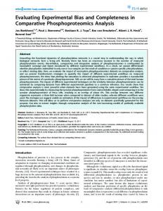
The last row of Table 2 shows that the realistic setting, where training is temporally precedent to testing, causes the worst classifier performance in the majority of cases. For a time-aware view of performance decay over time, Figure 2 plots per-month performance against the testing period, measured as the offset in months from training set (from 1 to 24). We can see that performance naturally decays over time, in particular for the malware class (darker lines), due to the concept-drift of evolving malware. The settings in which these plots are generated are presented in §4.

3.3

Spatial Experimental Bias

We identify two main types of spatial experimental bias based on assumptions on percentages of malware in testing and training sets. All experiments in this section assume temporal consistency. The model is trained on 2014 and tested on 2015 and 2016 (as in the

7 Alg1

[4] relies on hold-out by performing 10 random splits (66% training and 33% testing). Since the hold-out approach is very similar to k-fold CV and suffers from the same space-time biases, for the sake of simplicity we refer to k-fold CV setting for both Alg1 and Alg2.

4

1.0

1.0

1.0

1.0

0.9

0.9

0.9

0.9

0.8

0.8

0.8

0.8

0.7

0.7

0.7

0.7

0.6

0.6

0.6

0.6

0.5

0.5

0.5

0.5

0.4

0.4

0.4

0.3

0.3

0.3

0.2

0.2

0.2

0.1

0.1

0.4

F1 (mw) Precision (mw) Recall (mw) F1 (gw) Precision (gw) Recall (gw)

0.3 0.2 0.1 0.0

10%

25% 50% 75% %mw (Testing set)

90%

(a) Alg1: Training with 10% mw

0.0

10%


0.0

90%

(b) Alg1: Training with 90% mw

0.1 10%


90%

(c) Alg2: Training with 10% mw

0.0

10%


90%

(d) Alg2: Training with 90% mw

Figure 3: Experimental bias in testing. Training on 2014 and testing on 2015 and 2016. For increasing percentage of malware in the testing (unrealistic setting), Precision for malware increases and Recall remains the same; overall, F 1 -Score increases for increasing percentage of malware in the testing. However, having more malware than goodware in testing does not reflect the in-the-wild distribution of 10% malware (§2.2), so the setting with more malware is unrealistic and reports biased results.

Experimental bias in training. The percentage of malware in testing must be representative of the real in-the-wild distribution, but what about training? To understand the impact of altering malware-to-goodware ratios in training, we now consider a motivating example with a linear SVM in a 2D feature space, with features x 1 and x 2 . Figure 4 reports three scenarios, all with the same test distribution with 10% class 1 elements (e.g., mw in §2.2), but different percentages of class 1 in training: 10%, 50%, 90%. We can observe that with an increasing percentage of malware in training, the hyperplane moves towards class 0 (e.g., gw). More formally, it improves Recall of class 1 while reducing its Precision. The opposite is true for class 0. To minimize the overall error rate Err = F P + F N /(T P + T N + F P + F N ) (i.e., maximize Accuracy), one should train the dataset with the same distribution that is expected in the testing. However, in this scenario one may have more interest in finding more objects of the minority class (e.g., “more malware”) by improving Recall subject to a constraint on maximum FPR. Figure 5 shows the performance for Alg1 and Alg2, for increasing percentages of malware in training on the X -axis; just for completeness (since one cannot change artificially the test distribution to achieve realistic evaluations), we report results both for 10% mw in testing and for 90% malware in testing, but we remark that in the Android setting we have 10% mw in the wild (§2.2). These plots confirm the trend in our motivating example (Figure 4), that is, Rmw increases but Pmw decreases. For the plots with 10% mw in testing, we observe there is a point in which F 1 -Scoremw is maximum while the error for the goodware class is within 5%. In §4.3, we propose a novel algorithm to improve the performance of the malware class according to the objective of the user (high Precision, Recall or F 1 -Score), subject to a maximum tolerated error. Moreover, in §4 we introduce constraints and metrics that

last row of Table 2) to allow the analysis of spatial bias without the interference of time bias. Experimental bias in testing. The percentage of malware in the testing distribution needs to be estimated (§2.2) and cannot be changed, if one wants results to be representative of in-the-wild deployment of the malware classifier. To understand why this biases results, we artificially vary the testing distribution to illustrate our point. Figure 3 reports performance (F 1 -Score, Precision, Recall) for increasing the percentage of malware during testing on the X -axis. We change the percentage of malware in the testing set by randomly downsampling goodware, so the number of malware remains fixed throughout the experiments.8 For completeness, we report the two training settings from Table 2 with 10% and 90% malware, respectively. Let us first focus on the malware performance (dashed lines). All plots in Figure 3 exhibit constant Recall, and increasing Precision for increasing percentage of malware in the testing. Precision for the malware (mw) class—the positive class—is defined as Pmw = T P/(T P + F P ) and Recall as Rmw = T P/(T P + F N ). In this scenario, we can observe that TPs (i.e., malware objects correctly classified as malware) and FNs (i.e., malware objects incorrectly classified as goodware) do not change, because the number of malware does not increase; hence, Recall remains stable. The increase in number of FPs (i.e., goodware objects misclassified as malware) decreases as we reduce the number of goodware in the dataset; hence, Precision improves. Since the F 1 -Score is the harmonic mean of Precision and Recall, it goes up with Precision. We also observe that, on the opposite, the Precision for the goodware (gw) class—the negative class—Pдw = T N /(T N + F N ) decreases (see yellow solid lines in Figure 3), because we are reducing the TNs while the FNs do not change. This example shows how considering an unrealistic testing distribution with more malware than goodware (§2.2) positively inflates Precision and hence the F 1 -Score of the malware classifier.8

increase because TPs would increase for any mw detection, and FPs would not change— because the number of gw remains the same; if training (resp. testing) observations are sampled from a distribution similar to the mw in the original dataset (e.g., new training mw is from 2014 and new testing mw comes from 2015 and 2016), then Recall (Rmw = T P/(T P + F N )) would be stable—it would have the same proportions of TPs and FNs because the classifier will have a similar predictive capability for finding malware. Hence, if the number of malware in the dataset increases, the F 1 -Score would increase as well, because Precision increases while Recall remains stable.

8 We

choose to downsample goodware to achieve up to 90% of malware for testing because of the computational and storage resources required to achieve such a ratio by oversampling. This does not alter the conclusions of our analysis. Let us assume a scenario in which we keep the same number of gw, and increase the percentage of mw in the dataset by oversampling mw. The precision (Pmw = T P/(T P + F P )) would

5

0.5 gw mw

0.0 0.0

0.2

0.4

0.6 x1

0.8

1.0 x2

1.0 x2

x2

1.0

0.5 gw mw

0.0

1.0

0.0

(a) Training 10% mw; Testing 10% mw

0.2

0.4

0.6 x1

0.8

0.5 gw mw

0.0

1.0

0.0

(b) Training 50% mw; Testing 10% mw

0.2

0.4

0.6 x1

0.8

1.0

(c) Training 90% mw; Testing 10% mw

Figure 4: Motivating example for intuition of experimental bias in training with Linear-SVM and two features, x 1 and x 2 . The training changes, but the testing points are fixed: 90% gw and 10% mw. When the percentage of malware in the training increases, the decision boundary moves towards gw class, improving Recall for malware but decreasing Precision.

1.0

1.0

1.0

1.0

0.9

0.9

0.9

0.9

0.8

0.8

0.8

0.8

0.7

0.7

0.7

0.7

0.6

0.6

0.6

0.6

0.5

0.5

0.5

0.5

0.4

0.4

0.4

0.3

0.3

0.3

0.2

0.2

0.2

0.1

0.1

0.4

F1 (mw) Precision (mw) Recall (mw) F1 (gw) Precision (gw) Recall (gw)

0.3 0.2 0.1 0.0

10%

25% 50% 75% %mw (Training set)

90%

0.0

(a) Alg1: Testing with 10% mw

10%


0.0

90%

(b) Alg1: Testing with 90% mw

0.1 10%


90%

(c) Alg2: Testing with 10% mw

0.0

10%


90%

(d) Alg2: Testing with 90% mw

Figure 5: Experimental bias in training. Training on 2014 and testing on 2015 and 2016. For increasing percentage of malware in the training, Precision decreases and Recall increases, for the motivations illustrated in the toy example of Figure 4. In §4.3, we devise an algorithm to find the best training configuration for optimizing Precision, Recall, or F 1 -Score (depending on user needs). all the evaluations and tuning algorithms must assume that labels yi of objects si ∈ Ts are unknown. To evaluate performance over time, the test set Ts must be split into time-slots of size ∆. For example, for a testing set time window of size S = 2 years, we may have ∆ = 1 month. This parameter is chosen by the user, but it is important that the chosen granularity allows to have a statistically significant number of objects in any test window [ti , ti + ∆). We now formalize three constraints that must be enforced when dividing D into Tr and Ts for a realistic evaluation setting that avoids space-time experimental bias (§3). While C1 was proposed in past [2, 29], we are the first to propose C2 and C3.

enforce realistic experimental settings without space-time bias and produce results that allow comparisons among different algorithms.

4

SPACE-TIME AWARE EVALUATION

We now formalize how to perform an evaluation of a malware classifier free from space-time bias. We define a novel set of constraints that must be followed for realistic evaluations (§4.1); then, we introduce a novel time-aware metric, AUT, that captures in one number the impact of time decay on a classifier (§4.2); finally, we propose a novel tuning algorithm that empirically optimizes a classifier performance, subject to a maximum tolerated error (§4.3).

4.1

Evaluation Constraints

C1) Temporal training consistency. All the objects in the training must be strictly temporally precedent to the testing ones:

Let us consider D as a labeled dataset with two classes: malware (positive class) and goodware (negative class). Let us define si ∈ D as an object (e.g., an application) with timestamp time(si ). To evaluate the classifier, the dataset D must be split into a training dataset Tr with a time window of size W , and a testing dataset Ts with a time window of size S. If enough data is available (e.g., three years), we recommend to consider S > W , in order to estimate long-term performance and robustness to decay of the classifier. We observe that, although we know the labels of objects in Ts ⊆ D,

time(si ) < time(s j ), ∀si ∈ Tr, ∀s j ∈ Ts

(1)

where si (resp. s j ) is an object in the training set Tr (resp. testing set Ts). Eq. 1 must hold; its violation inflates the results by including future knowledge in the classifier (§3.2). 6

Algorithm 1: Tuning φ.

C2) Temporal gw/mw windows consistency. In every testing slot of size ∆, all test objects must be from the same time window: timin ≤ time(sk ) ≤ timax , ∀sk ∈ objects in time slot [ti , ti + ∆) where timin

(2)

1

mink time(sk ) and timax

= = maxk time(sk ). This constraint has been violated in the past when goodware and malware have been collected from different time windows (e.g., [27])—if violated, the results are biased because the classifier may learn behaviors that distinguish applications from different time windows. C3) Realistic malware-to-goodware percentage in testing. The testing distribution must reflect the real-world percentage of malware observed in the wild to avoid inflating results (§3.3). More formally, let us define φ as the average percentage of malware in training data, and δ as the average percentage of malware in the testing data. Let σˆ be the estimated percentage of malware in the wild. Then, we would like to have: δ = σˆ

2

3 4 5 6 7 8 9 10 11 12 13 14

(3) the performance curve over time. More formally, based on the trapezoidal rule9 , AUT is defined as follows:

which means that the average percentage of malware in the test distribution (δ ) must be as close as possible to the percentage of malware in the wild (σˆ ). For example, we have estimated that in the Android scenario goodware is predominant over malware, with σˆ ≈ 0.10 (§2.2). If C3 is violated, the results are positively inflated (§3.3). We highlight that, although the testing distribution δ cannot be changed (in order to get realistic results constraint C3), the percentage of malware in the training φ may be tuned (§4.3).

4.2

Input: Training dataset T r Parameters : Learning rate µ , target performance P ∈ {F 1, P r, Rec }, max error rate Emax Output: φ P∗ , optimal percentage of mw to use in training to achieve the best target performance P subject to E < Emax . Split the training set Tr into two subsets: actual training (ProperTr) and validation set (Val), while enforcing C1, C2, C3 (§4.1), also implying δ = σˆ Divide Val into N non-overlapped subsets, each corresponding to a time-slot ∆, so that Val ar r ay = [V0, V1, ..., VN ] Train a classifier Θ on ProperTr P ∗ ← AUT(P, N ) on Val ar r ay with Θ φ P∗ = σˆ for (φ = σˆ ; φ ≤ 0.5; φ = φ + µ ) do Downsample gw in ProperTr so that percentage of mw is φ Train the classifier Θφ on ProperTr with φ mw performance Pφ ← AUT(P, N ) on Val ar r ay with Θφ error Eφ ← Error rate on Val ar r ay with Θφ if ( Pφ > P ∗ ) and ( Eφ ≤ Emax ) then P ∗ ← Pφ φ P∗ ← φ return φ P∗ ;

AUT (f , N ) =

N −1 1 Õ [f (x k +1 ) + f (x k )] · (1/N ) N −1 2

(4)

k =1

where: • f (x k ) is the value of the point estimate of the performance metric f (e.g., F 1 -Score) evaluated at point x k . • The X -axis coordinate x k := (W + k∆) • N is the number of test slots, and 1/(N −1) is a normalization factor so that AUT ∈ [0, 1] • N1−1 is the normalization factor The perfect classifier with robustness to time decay has AUT = 1. By default, AUT is computed as area under point estimates, as they capture more closely the trend of the classifier over time; if the AUT is computed on cumulative estimates, it should be explicitly marked as AUTcml . As an example, AUT (F 1 , 12m) is the point estimate of F 1 -Score considering time decay for a period of 12 months, with a 1-month interval. It is important to observe that, as long as the X -axis is normalized between 0 and 1, the AUT does not directly depend on ∆.

Time-aware Performance Metrics

We introduce a time-aware performance metric that allows to compare the results of different classifiers while considering time decay. Let Θ be a classifier trained on Tr; we capture the performance of Θ for each time frame [ti , ti +∆) of the testing set Ts (e.g., each month). We identify two options to represent per-month performance: • Point estimates (pnt): The value plotted on the Y -axis for x k = k∆ (where k is the test slot number) computes the performance metric (e.g., F 1 -Score) only based on predictions yˆi of Θ and true labels yi in the interval [W +(k−1)∆,W +k∆). • Cumulative estimates (cml): The value plotted on the Y axis for x k = k∆ (where k is the test slot number) computes the performance metric (e.g., F 1 -Score) only based on predictions yˆi of Θ and true labels yi in the cumulative interval [W ,W + k∆).

AUT is a metric that allows us to evaluate performance of a malware classifier against time decay in realistic experimental settings—obtained by enforcing C1, C2, and C3 (§4.1). The next sections leverage AUT for tuning classifiers and comparing different solutions.

Point estimates are preferred to represent the real trend of the classifier when enough data is available for each test slot ∆; if many slots ∆ are only sparsely populated with objects (or if their number is highly variable), then cumulative estimates must be preferred, as they smooth the trend. An example of cumulative plot is reported in Appendix A.2. Figure 2 (§3.1) shows the point estimate of time decay for Alg1 and Alg2, where the X -axis reports the time-shift k, and each time-slot ∆ has size 1 month. Without loss of generality, since our dataset has enough objects in each slot (see §2.3) we report only point estimates in the remainder of the paper. To facilitate the comparison of different time decay plots, we define a new metric, AUT (Area Under Time), the area under the

4.3

Tuning Training Ratio

We propose a novel algorithm that allows for the adjustment of the training ratio φ when the dataset is imbalanced, in order to optimize a user-specified performance metric (F 1 , Precision, or Recall) on the minority class, subject to a maximum tolerated error. The high-level intuition of the impact of changing φ is described in §3.3. 9 The

trapezoidal rule is also used by the AUC [6] metric to measure the area under ROC curve.

7

Table 3: Testing AUTs performance over 24 months when ∗ . training with σˆ , φ ∗F , φ ∗P r and φ Rec

Our tuning algorithm is inspired by the one proposed by Weiss and Provost [44]; they propose a progressive sampling of training objects to collect a dataset that improves AUC performance of the minority class in an imbalanced dataset. However, they did not take temporal constraints into account (§3.2), and can only optimize AUC heuristically. Conversely, we enforce C1, C2, C3 (§4.1), and rely on AUT to achieve three possible targets for the malware class: higher F 1 -Score, higher Precision, or higher Recall. Also, we assume that the user already has a training dataset Tr and wants to use as many objects from it as possible, while still achieving a good performance trade-off; for this purpose, we perform a progressive subsampling of the goodware class. Algorithm 1 presents our methodology for tuning the parameter φ to find the value φ P∗ that optimizes P subject to a maximum error rate E. The algorithm aims to solve the following optimization problem:

1

Algorithm

AUT(P,24m) F1 Pr Rec

FP

FN

Alg1 [4]

10% (σˆ ) 25% (φ F∗ ) 1 10% (φ P∗ r ) ∗ ) 50% (φ Rec

965 2,156 965 3,728

3,851 2,815 3,851 1,793

0.58 0.63 0.58 0.64

0.75 0.65 0.75 0.58

0.48 0.61 0.48 0.74

Alg2 [27]

10% (σˆ ) 50% (φ F∗ ) 1 10% (φ P∗ r ) ∗ 50% (φ Rec )

274 4,160 274 4,160

5,689 2,689 5,689 2,689

0.30 0.53 0.30 0.53

0.77 0.50 0.77 0.50

0.20 0.60 0.20 0.60

φ ∗F = 0.25 for Alg1 and φ ∗F = 0.5 for Alg2. Figure 6(a) shows the 1 1 trade-off between AUT and error rate from the validation, used ∗ to estimate φ F with Algorithm 1; then, Figure 6(b) reports the 1 impact on the test-time performance of applying φ ∗F to the full 1 training set Tr . We remark that the choice of φ ∗F uses only training 1 information (see Algorithm 1) and no test information is used—this is to simulate a realistic deployment setting in which we have no a priori information about testing. Figure 6 shows that our approach for finding the best φ ∗F improves the F 1 -Score on malware at test 1 time, at a reduced cost on goodware performance. Table 3 shows details of how FP, FN, and AUT changed by training Alg1 and ∗ Alg2 with φ ∗F , φ ∗P r ec , and φ Rec instead of σˆ ; as expected (§3.3), 1 ∗ when training with φ F Precision decreases (FPs increase) but Recall 1 increases (because FNs decrease), and the overall AUT increases slightly as a trade-off. A similar reasoning follows for the other performance targets.

maximizeφ {P} subject to: E ≤ Emax

φ

(5)

where P is the target performance: the F 1 -Score (F 1 ), Precision (Pr ) or Recall (Rec) of the malware class; Emax is the maximum tolerated error; depending on the target P, the error rate E has a different formulation: • if P = F 1 , E = 1 − Accuracy = (F P + F N )/(T P + T N + F P + F N ) • if P = Rec, E = F PR = F P/(T N + F P ) • if P = Pr , E = F N R = F N /(T P + F N ) Each of these definitions of E is targeted to limit the error induced by the specific performance—if we want to maximize F 1 for the malware class, we need to limit both FPs and FNs; if P = Pr , we increase FNs, so we constrain FNR (see also §3.3). Algorithm 1 consists of two phases: initialization (lines 1–5) and grid search of φ P∗ (lines 6–14). In the initialization phase, the training set T r is split into a proper training set ProperTr and a validation Val; this is split according to the space-time evaluation constraints in §4.1, so that all the objects in ProperTr are temporally anterior to Val, and the malware percentage δ in Val is equal to σˆ , the in-thewild malware percentage. The maximum performance observed P ∗ and the optimal φ P∗ are initialized by assuming the estimated in-the-wild malware distribution σˆ ; in our scenario, σˆ = 10% (see §2.2). The grid-search phase iterates over different values of φ, with a learning rate µ (e.g., µ = 0.05), and keeps as φ P∗ the value leading to the best performance, subject to the error constraint. To reduce the chance of discarding high-quality points while downsampling goodware, we prioritize the most uncertain points (e.g., points close to the decision boundary in an SVM) [38]. The constraint on line 6 (σˆ ≤ φ ≤ 0.5) is to ensure that one does not under-represent the minority class (if φ < σˆ ) and that one does not let it become the majority class (if φ > 0.5); also, from §3.3 it is clear that if φ > 0.5, then the error rate becomes too high for the goodware class. Finally, the grid-search explores multiple values of φ and stores the best ones. To capture time-aware performance, we rely on AUT (§4.2), and the error rate is computed according to the target P (see above). Let us consider an example on our dataset. We want to maximize P = F 1 -Score of malware class, subject to Emax = 10%. After running Algorithm 1 on Alg1 [4] and Alg2 [27], we find that

5

DELAYING TIME DECAY

Certain machine learning techniques can improve the robustness of a classifier against time decay; for example, by adding an extra class, “rejected”, for uncertain classifications (classification with reject option [20]), or by retraining after relabeling a subset of objects (active learning [38]). However, this performance improvement comes at a cost. In this section, we show how our constraints and AUT allows to compare performance-cost trade-offs for different approaches to the time decay problem. We stress that the main contribution of this section is to show preliminary experiments on viable directions of future work. We do not propose any novel active learning or classification with rejection algorithm; we instead show how our metrics and constraints can be used to evaluate and compare the impact of such approaches.

5.1

Performance-cost Trade-off

Some approaches are capable of improving performance without changing the internals of the classifier (i.e., feature space and decision algorithm); however, this comes at a cost. To quantify performance-cost trade-offs of methods to delay time decay without changing the algorithm, we characterize the following elements: • Performance (P): The performance measured in AUT to capture robustness against time decay (§4.2). 8

Alg1

1.0 0.9

Alg2

1.0

AUT(F1, 4 months) Error rate

Alg1

1.0

Alg2

1.0

0.9

0.9

0.9

0.8

0.8

0.8

0.8

0.7

0.7

0.7

0.7

0.6

0.6

0.6

0.6

0.5

0.5

0.5

0.5

0.4

0.4

0.4

0.4

0.3

0.3

0.3

0.2

0.2

0.2

0.1

0.1

0.1

0.0

0.0

0.0

0.3

F1 (mw, σ ˆ)

5

15

25

35

45

55

65

75

85

95

5

15

%mw (Training set)

25

35

45

55

65

75

85

0.1

F1 (gw, ϕ∗ )

0.0 1

95

0.2

F1 (mw, ϕ∗ ) F1 (gw, σ ˆ

4

7

10

13

16

19

22

1


%mw (Training set)

(a) Choosing φ F∗ from validation performance

4

7

10

13

16

19

22


(b) Effect of φ = φ F∗ and φ = σˆ at test-time

1

1

Figure 6: Improvement obtained by applying φ ∗F = 25% to Alg1 and φ ∗F = 50% for Alg2. The values of φ ∗F have been obtained 1 1 1 with Algorithm 1 run on the training data of one year.

Alg1

1.0 0.9

0.9

0.8

0.8

0.7

0.7

0.6

0.6

0.5

0.5

0.4

line represents the F 1 -Score without incremental retraining (i.e., stationary training). The low performance in the last 2-3 months of the plots is related to the lesser quantity of objects available in those periods (§2.3). Although incremental retraining generally achieves optimal performance throughout the whole test period, it also incurs the highest relabeling cost R.

Alg2

1.0

0.4

F1 (10-fold CV)

0.3

0.3

5.3

F1 (no update) 0.2

0.2


0.1

0.1

F1 (mw)

0.0

0.0 1

4

7

10

13

16

19

22

1


4

7

10

13

16

19

22


Figure 7: Delaying time decay: incremental retraining.

• Relabeling cost (R): The number of testing objects (if any) that must be relabeled; the relabeling must occur periodically (e.g., every month), and is particularly costly in the malware domain as manual inspection requires many resources (infrastructure, time, expertise, etc). • Quarantine cost (Q): The number of objects (if any) rejected by the classifier; they must be manually verified, so there is a cost associated with leaving them in quarantine. The following subsections evaluate some practical approaches which can be used to defer time decay; we subsequently analyze their performance-cost trade-offs with Tesseract.

5.2

Active Learning

Active learning is a field of machine learning that studies query strategies to select a small number of testing points close to the decision boundaries, that, if included in the training set, are the most relevant for updating the classifier. For example, in a linear SVM the slope of the decision boundary greatly depends on the points that are closest to it, the support vectors [6]; all the points further from the SVM decision boundary are classified with higher confidence, hence have limited effect on the slope of the hyperplane. We evaluate the impact of one of the most popular active learning strategies: uncertainty sampling [29, 38]. This query strategy selects the most points the classifier is least certain about, and uses them for retraining; we apply it in a time-aware scenario, and choose a percentage of objects to retrain per month. The intuition is that the most uncertain elements are the ones that may be indicative of concept-drift, and new, correct knowledge about them may better inform the decision boundaries. The number of objects to relabel depends on the user’s available resources for relabeling. For example, Miller [29] estimated that an average company could manually relabel 80 objects per day. More formally, in binary classification uncertainty sampling ∗ (where LC stands for Least Confident) to each gives a score x LC sample [38]; this score is defined as follows10 :

Incremental Retraining

We first consider an approach that tends towards an “ideal” performance P ∗ : incremental retraining, whereby all test objects are periodically relabeled manually, and the new knowledge introduced to the classifier via retraining. Figure 7 shows the performance of Alg1 and Alg2 with monthly incremental retraining. More formally, the performance of month mi is determined from the predictions of Θ trained on: T r ∪ {m 0 , m 1 , ..., mi−1 }, where {m 0 , m 1 , ..., mi−1 } are testing objects, which are manually relabeled. The dashed gray

∗ ˆ x LC := argmaxx {1 − P Θ (y|x)}

(6)

where yˆ := argmaxy PΘ (y|x) is the class label with the highest posterior probability according to classifier Θ. In a binary classification 10 In

multi-class classification, there is a query strategy based on the entropy of the prediction scores array; in binary classification, the entropy-based query strategy is proven to be equivalent to the “least confident” [38].

9

with σˆ and φ ∗F , respectively. In each row, we highlight in purple 1 cells (resp. orange) the column with the highest AUT for Alg2 (resp. Alg1). The table allows us to:

Table 4: Performance-cost comparison of delay methods. Costs R Delay method No update Rejection (σˆ ) Rejection (φ F∗ ) 1 AL: 1% AL: 2.5% AL: 5% AL: 7.5% AL: 10% AL: 25% AL: 50% Inc. retrain

Q

Performance P φ = σˆ φ = φ F∗ 1 Alg1 Alg2 Alg1 Alg2

Alg1

Alg2

Alg1

Alg2

0

0

0

0

0.577

0.305

0.622

0.527

0 0 709 1,788 3,589 5,387 7,189 17,989 35,988 71,988

0 0 709 1,788 3,589 5,387 7,189 17,989 35,988 71,988

10,283 10,576 0 0 0 0 0 0 0 0

3,595 24,390 0 0 0 0 0 0 0 0

0.717 – 0.708 0.738 0.782 0.793 0.796 0.821 0.817 0.818

0.280 – 0.456 0.509 0.615 0.641 0.656 0.674 0.679 0.679

– 0.704 0.703 0.758 0.784 0.801 0.802 0.823 0.828 0.830

– 0.683 0.589 0.667 0.680 0.714 0.732 0.732 0.741 0.736

• examine the effectiveness of the training ratios φ ∗F and σˆ ; 1 • analyze the performance improvement in terms of AUT and the corresponding cost from delaying time decay; • and compare the performance of Alg1 and Alg2 in different settings. First, let us compare φ ∗F with σˆ . The first row of Table 4 repre1 sents the scenario in which the model is trained only once at the beginning—the scenario for which we originally designed Algorithm 1 (§4.3 and Figure 6). Without methods to delay time decay, φ ∗F achieves better performance than σˆ for both Alg1 and Alg2 1 at no cost. In all other configurations, we observe that training φ = φ ∗F always improves performance for Alg2, whereas for Alg1 1 it is slightly advantageous in most cases except for rejection and AL 1%—in general, the performance of Alg1 trained with φ ∗F and σˆ is 1 consistently close. The intuition for this outcome is that φ ∗F and σˆ 1 are also close for Alg1: when applying the AL strategy, we re-apply at each step Algorithm 1 and we find that the average φ ∗F ≈ 15% 1 for Alg1, which is close to 10% (i.e., σˆ ). On the other hand, for Alg2 the average φ ∗F ≈ 50%, which is far from σˆ and improves all results 1 significantly. We can conclude that our algorithm for tuning the training is most effective when it finds a φ P∗ that differs from the estimated σˆ . Then, we analyze the performance improvement and related cost of using delay methods. The improvement granted by our algorithm in F 1 -Score comes at no relabeling or quarantine cost. We can observe that one can improve the in-the-wild performance of the algorithms at some cost R or Q. It is important to observe that objects discarded or to be relabeled are not necessarily malware; they are just the objects most uncertain according to the algorithm, which the classifier may have likely misclassified. The relabeling costs R for Alg1 and Alg2 are identical as both operate on the same dataset (§2.3); in active learning, the percentage of retrained objects is user-specified and fixed. In Table 2, the cells with the red background reported the performance of Alg1 and Alg2 in settings considered in their own papers [4, 27]; from the biased settings, it may seem that Alg2 performs better than Alg1. However, after using Tesseract to eliminate space-time experimental bias, we find out that the performance of both classifiers is lower in realistic settings, but that Alg1 is likely to perform better than Alg2. This holds also in Table 4, which demonstrates that Alg1 outperforms Alg2 on F 1 -Score for all performance-cost trade-offs. Tables such as Table 4 can be generated by Tesseract (§6) and should be helpful to both researchers and industrial practitioners. Practitioners need to understand the performance of a classifier in the wild, compare different algorithms, and determine the resources required for R and Q. For researchers, it is useful to understand how to reduce the costs R and Q while improving the performance P of classifiers and producing comparable, unbiased evaluations. This problem is challenging, but we hope that the release of Tesseract’s source code (§6) fosters further research and a widespread adoption.

task, the maximum uncertainty for an object is achieved when its prediction probability equal to 0.5 for both classes (i.e., equal probability of being goodware or malware). The test objects are sorted by ∗ , and the top-n most uncertain descending order of uncertainty x LC are selected to be relabeled for retraining the classifier. Figure 8 reports the results obtained by applying Active Learning (AL) with uncertainty sampling, for different percentage of objects relabeled per month. Each scenario corresponds to a different cost R. We observe that even with 1% AL, the performance already improve significantly; this is because the assumption that the most uncertain objects are the ones that may move the decision boundary over time is empirically verified. The relabeling cost R is known a-priori since it is user specified.

5.4

Classification with Reject Option

Malware evolves rapidly over time, so if the classifier is not up to date, the decision region may no longer be representative of new objects. Another approach, orthogonal to active learning, is to include a reject option as a possible classifier outcome [14, 20]. This discards the most uncertain predictions to a quarantine area for manual inspection at a future date. At the cost of rejecting some objects, the overall performance of the classifier (on the remaining objects) increases. The intuition is that in this way only high confidence decisions are taken into account. Figure 9 reports the performance of Alg1 and Alg2 after applying a reject option based on [20].11 The gray histogram on the background reports number of rejected objects per each month. We observe that the second year of testing has more rejected objects for both Alg1 and Alg2, although Alg2 overall is rejecting more objects. Again, although performance P improves, there is a quarantine cost Q associated with it; unlike active learning, in this case the cost is not known a-priori, because in traditional classification with rejection, a threshold on the classifier confidence is applied [14, 20].

5.5

Analysis of Delay Methods

Table 4 is built with AUT on F 1 (§4.2) and by enforcing our constraints and reports a summary of relabeling cost R, quarantine cost Q, and two performance columns P, corresponding to training 11 In

particular, we use the third quartile of probabilities of incorrect predictions as rejection threshold [20].

10

Alg1

1.0

Alg2

1.0

Alg1

1.0

Alg2

1.0

Alg1

1.0

0.9

0.9

0.9

0.9

0.9

0.8

0.8

0.8

0.8

0.8

0.8

0.7

0.7

0.7

0.7

0.7

0.7

0.6

0.6

0.6

0.6

0.6

0.6

0.5

0.5

0.5

0.5

0.5

0.5

0.4

0.4

0.4

0.4

0.4

0.3

0.3

0.3

0.3

0.2

0.2

0.2

0.2

0.1

0.1

0.1

0.1

0.3

25% 10% 5% 1% 0%

0.2 0.1 0.0

0.0

0.0 1

4

7

10

13

16

19

22

25% 10% 5% 1% 0%

1

4


7

10

13

16

19

4

7

10

13

16

19

22

1



(a) F 1 -Score

0.4 0.3

25% 10% 5% 1% 0%

0.2 0.1

0.0

0.0 1

22

4

7

10

13

16

19

22


Alg2

1.0

0.9

0.0 1

4

7

10

13

16

19

22

1


(b) Precision

4

7

10

13

16

19

22


(c) Recall

Figure 8: Performance with active learning with uncertainty sampling. Alg1

1.0

2600

Alg2

1.0

2400

0.9

2400

2200 0.8

2200 0.8

2000

0.7

1600

F1 (no rejection) Recall (gw)

0.5

1400

Precision (gw)

1200

0.4

F1 (gw) Recall (mw)

1000

0.3

Precision (mw)

800 600

F1 (mw)

0.2

2000

0.7

1800

0.6

1600 1400

0.5

1200

0.4

1000

0.3

800 600

0.2

400 0.1

200

0.0

0 1

4

7

10

13

16

19

22


# Quarantined

0.6

# Quarantined

1800

metrics.py. As Tesseract aims to encourage comparable and reproducible evaluations, we include functions for visualizing classifier assessments and operating on the results returned by the predict() family of functions. This enables the user to easily derive metrics such as the total errors or accuracy from slices of a time-aware evaluation. Importantly we also include aut() for computing the AUT for a given metric (F 1 , Precision, AUC, etc.) over a given time period. active.py and reject.py. We incorporate implementations of the model update methods discussed in §5 and integrate them into the time-aware evaluation using a modular design that allows novel query and reject strategies to be easily plugged in. We hope this lowers the bar for follow-up research in these areas. The source code of Tesseract is available for download. We also make available the SHA256 hashes of all apps in the raw datasets used in the experiments (SHA256 hash digest), which allows to reproduce our samples from AndroZoo. Finally, we release all metadata and feature sets extracted by running Alg1 and Alg2.

2600

0.9

400 0.1

200 0

0.0 1

4

7

10

13

16

19

22


Figure 9: Delay time decay: classification with rejection.

6

IMPLEMENTATION

We have implemented our constraints, metrics, and algorithms as a Python library named Tesseract, designed to integrate easily with common workflows. In particular, the API design of Tesseract is heavily inspired by and fully compatible with the popular machine learning library Scikit-learn [32]. As a result, many of the conventions and workflows in Tesseract will be familiar to Scikit-learn users. An overview of the library’s core modules follows:

7

DISCUSSION

We now discuss our assumptions and how we address limitations of our work. Domain-specific in-the-wild malware percentage σˆ . In the Android landscape, we assume that σˆ is around 10% (see §2.2). Correctly estimating the malware percentage in the testing dataset is a challenging task and we encourage further representative measurement studies [24, 43] and data sharing to obtain realistic experimental settings to promote the unbiased evaluation of machine learning-based malware classification techniques. Correct observation labels. We assume goodware and malware labels in the dataset are correct (§2.3). Similarly, we consider relabeling tasks in active learning (§5) to be correct as well. It is worth mentioning that Miller et al. [29] found that AVs sometimes change their outcome over time; in particular, some goodware may eventually be tagged as malware. However, Miller et al. [29] also found that VirusTotal detections stabilize after one year; since we are using observations up to Dec 2016, we consider VirusTotal’s labels as reliable. In the future, we may integrate approaches for noisy oracles [12], which assume some observations are mislabeled. Correct observation timestamps. We rely on the dex_date as the approximation of an observation timestamp, as recommended

temporal.py. While machine learning libraries commonly involve working with a set of predictors X and a set of output variables y, Tesseract extends this concept to include an array of datetime objects t. This allows for operations such as the timeaware partitioning of datasets (e.g., time_aware_partition() and time_aware_train_test_split()) while respecting temporal constraints C1 and C2. Also central to the module are the predict() and fit_predict() functions that accept a classifier, dataset and set of parameters (as defined in §4.1) and return the results of a time-aware evaluation performed across the chosen periods. spatial.py. This module allows the user to alter the proportion of the positive class in a given dataset. downsample_set() can be used to simulate the natural class distribution σˆ expected during deployment or to tune the performance of the model by over-representing a class during training. To this end we provide an implementation of Algorithm 1 for finding the optimal training proportion φ ∗ (search_optimal_train_ratio()). This module can also assert that spatial constraint C3 (§4.1) has not been violated. 11

and malicious traffic, even F PR = 0.1% would cause too many false positives per day (hundreds of thousands), so T PR = T P/T P + F N is not the right target metric to be looking for. This is also related to spatial bias given the imbalance in the dataset. In our evaluation framework, we do not suffer from the same base rate fallacy since we are also considering Precision, which will be extremely low for the minority class if there are many false positives; moreover, in the malware setting, the percentage of malware in the wild is about 510% (§2.2), whereas for malicious communications may be as small as 0.001% of total traffic [5]. Fawcett [13] focuses on challenges in spam detection, one of which resembles spatial bias; no solution is provided, whereas we introduce C3 to this end and demonstrate how its violation inflates performance. Torralba and Efros [42] discuss the problem of dataset bias in Computer Vision, different from our security setting where there are fewer benchmarks; in images the negative class (e.g., “not cat”) can grow arbitrarily, which is less likely in the malware context. Moreno-Torres et al. [31] systematize different drifts, and mention sample-selection bias; while this resembles spatial bias, [31] does not propose any solution/experiments for its impact on ML performance. The machine learning community has studied imbalanced datasets and highlighted how training and testing ratios can influence the results of an algorithm [7, 19, 44]. However, not coming from the security domain, these studies consider only spatial bias. In other applications, time is likely less problematic than in malware classification, which is plagued by concept drift [20]. Other related work underlines the importance of choosing appropriate performance metrics to avoid an incorrect interpretation of the results (e.g., ROC curves are misleading in an imbalanced dataset [11, 18]). In this paper, we take imbalance into account, and we aim to bring awareness to the security community of the issues and implications that these sources of space-time bias have in the relation to the scenario where the algorithm is going to operate.

by Allix et al. [3]. We further verified such an assumption by redownloading VirusTotal [16] reports for 25K apps and verifying that the first_seen attribute always matched the dex_date in our time span. To further improve the trustworthiness of the observations’ dates, one could verify whether a given observation contains time inconsistencies or features not yet available when the app was released (e.g., [40]). Resilience of malware classifiers. In our study, we analyze two recent high-profile classifiers. One could argue that other classifiers may show consistently high performance even with space-time bias eliminated. And this should indeed be the goal of research on malware classification. Tesseract provides a mechanism for an unbiased evaluation that we hope will support this kind of work. Adversarial machine learning. This work demonstrates the performance decay caused by concept drift in time-aware machine learning evaluations. Adversarial machine learning focuses on perturbing training or testing observations to compel a classifier to make incorrect predictions. Both relate to concepts of robustness and one can characterize adversarial machine learning as an artificially induced worst-case concept drift scenario. While the adversarial setting remains an open problem, the experimental bias we describe in this work—endemic in machine learning-based malware classification—must be addressed prior to realistic evaluations of adversarial mitigations.

8

RELATED WORK

We now compare our findings and solutions with related work on experiment design and bias in machine learning algorithms. Rossow et al [36] presented a set of best practice guidelines to help with the quality of experiments on malware classification. While helpful, these would be insufficient to prevent all sources of temporal and spatial bias we identify. Allix et al. [2] broke new ground by evaluating malware classifiers in relation to time and showing how future knowledge can inflate performance. As a separate issue, Allix et al. [1] investigated the difference between in-thelab and in-the-wild scenarios and found that the greater presence of goodware leads to lower performance. We systematically analyze and explain these issues and help to address them by formalizing a set of constraints, jointly considering the impact of temporal and spatial bias, and offering a tuning algorithm to leverage the effects of training data distribution. Miller et al. [29] identified temporal sample consistency (equivalent to our constraint C1), but not C2 or C3. In their approach, they considered the testing period to be a uniform time slot, whereas we take time decay into account. Roy et al. [37] questioned the use of recent or older malware as training objects and the performance degradation in testing real-world object ratios. Most experiments were designed without considering time, however, reducing the reliability of the conclusions. While past work highlighted some sources of experimental bias [1, 2, 36, 37], it gave little consideration to the goals of the classifier. Different scenarios have different goals (not necessarily maximizing the F 1 Score), therefore in our work we show the effects of different training settings on performance goals (§3) and propose a solution to properly tune the algorithm (§4.3). A common experimental bias in network intrusion detection is the base rate fallacy [5]: given the large imbalance between benign

9

AVAILABILITY

We make Tesseract’s code and data available to the research community and practitioners to promote the adoption of a sound and unbiased evaluation of machine learning in security contexts. Please send an email to Lorenzo Cavallaro for access information.

10

CONCLUSIONS

We propose a generic framework to highlight experimental bias and evaluate machine learning for malware detection with sound experiments that consider time decay and eliminate space-time bias. We define a set of constraints to enforce realistic evaluations and a novel metric, AUT, to summarize the time decay of a classifier. Defining AUT allowed us to propose a tuning algorithm that optimizes a target requirement (Precision, Recall, F 1 -Score) by changing the percentage of malware in the training set, without any relabeling cost to the user. To foster future research, we publicly release the code of Tesseract, a tool designed to evaluate any malware classifier without experimental space-time bias, and to enable a direct comparison of performance numbers while taking time decay into account. 12

REFERENCES

A APPENDIX A.1 Symbol table

[1] K. Allix, T. F. Bissyandé, Q. Jérome, J. Klein, R. State, and Y. Le Traon. Empirical Assessment of Machine Learning-Based Malware Detectors for Android. In Empirical Software Engineering, 2016. [2] K. Allix, T. F. Bissyandé, J. Klein, and Y. Le Traon. Are Your Training Datasets Yet Relevant? In ESSoS. Springer, 2015. [3] K. Allix, T. F. Bissyandé, J. Klein, and Y. Le Traon. Androzoo: Collecting Millions of Android Apps for the Research Community. In ACM Mining Software Repositories (MSR), 2016. [4] D. Arp, M. Spreitzenbarth, M. Hubner, H. Gascon, and K. Rieck. DREBIN: Effective and Explainable Detection of Android Malware in Your Pocket. In NDSS, 2014. [5] S. Axelsson. The Base-Rate Fallacy and the Difficulty of Intrusion Detection. ACM Transactions on Information and System Security (TISSEC), 2000. [6] C. M. Bishop. Pattern Recognition and Machine Learning. 2006. [7] N. V. Chawla, N. Japkowicz, and A. Kotcz. Special Issue on Learning From Imbalanced Data Sets. ACM SIGKDD Explorations Newsletter, 2004. [8] C. Curtsinger, B. Livshits, B. G. Zorn, and C. Seifert. ZOZZLE: Fast and Precise In-Browser JavaScript Malware Detection. In USENIX Security, 2011. [9] G. E. Dahl, J. W. Stokes, L. Deng, and D. Yu. Large-Scale Malware Classification Using Random Projections and Neural Networks. In IEEE Int. Conf. Acoustics, Speech and Signal Processing (ICASSP), 2013. [10] S. K. Dash, G. Suarez-Tangil, S. Khan, K. Tam, M. Ahmadi, J. Kinder, and L. Cavallaro. Droidscribe: Classifying Android Malware Based on Runtime Behavior. In MoST-SPW. IEEE, 2016. [11] J. Davis and M. Goadrich. The Relationship Between Precision-Recall and ROC Curves. In ICML, 2006. [12] J. Du and C. X. Ling. Active Learning with Human-Like Noisy Oracle. In ICDM, 2010. [13] T. Fawcett. In vivo spam filtering: a challenge problem for kdd. ACM SIGKDD Explorations Newsletter, 2003. [14] G. Fumera, I. Pillai, and F. Roli. Classification with reject option in text categorisation systems. In IEEE Int. Conf. Image Analysis and Processing, 2003. [15] H. Gascon, F. Yamaguchi, D. Arp, and K. Rieck. Structural Detection of Android Malware using Embedded Call Graphs. In ACM AISec, 2013. [16] Google. VirusTotal, 2004. [17] Google. Android Security 2017 Year In Review. https://source.android.com/ security/reports/Google_Android_Security_2017_Report_Final.pdf, March 2018. [18] D. J. Hand. Measuring Classifier Performance: a Coherent Alternative to the Area Under the ROC Curve. Machine Learning, 2009. [19] H. He and E. A. Garcia. Learning From Imbalanced Data. IEEE TKDE, 2009. [20] R. Jordaney, K. Sharad, S. K. Dash, Z. Wang, D. Papini, I. Nouretdinov, and L. Cavallaro. Transcend: Detecting Concept Drift in Malware Classification Models. In USENIX Security, 2017. [21] C. Kolbitsch, P. M. Comparetti, C. Kruegel, E. Kirda, X. Zhou, and X. Wang. Effective and Efficient Malware Detection at the End Host. In USENIX Security, 2009. [22] P. Laskov and N. Šrndić. Static Detection of Malicious JavaScript-Bearing PDF Documents. In ACSAC, 2011. [23] S. Lee and J. Kim. WarningBird: Detecting Suspicious URLs in Twitter Stream. In NDSS, 2012. [24] M. Lindorfer, S. Volanis, A. Sisto, M. Neugschwandtner, E. Athanasopoulos, F. Maggi, C. Platzer, S. Zanero, and S. Ioannidis. AndRadar: Fast Discovery of Android Applications in Alternative Markets. In DIMVA, 2014. [25] F. Maggi, A. Frossi, S. Zanero, G. Stringhini, B. Stone-Gross, C. Kruegel, and G. Vigna. Two Years of Short URLs Internet Measurement: Security Threats and Countermeasures. In WWW, 2013. [26] D. Maiorca, G. Giacinto, and I. Corona. A Pattern Recognition System for Malicious PDF Files Detection. In Intl. Workshop on Machine Learning and Data Mining in Pattern Recognition. Springer, 2012. [27] E. Mariconti, L. Onwuzurike, P. Andriotis, E. De Cristofaro, G. Ross, and G. Stringhini. MaMaDroid: Detecting Android Malware by Building Markov Chains of Behavioral Models. In NDSS, 2017. [28] Z. Markel and M. Bilzor. Building a Machine Learning Classifier for Malware Detection. In Anti-malware Testing Research (WATeR) Workshop. IEEE, 2014. [29] B. Miller, A. Kantchelian, M. C. Tschantz, S. Afroz, R. Bachwani, R. Faizullabhoy, L. Huang, V. Shankar, T. Wu, G. Yiu, et al. Reviewer Integration and Performance Measurement for Malware Detection. In DIMVA. Springer, 2016. [30] B. A. Miller. Scalable Platform for Malicious Content Detection Integrating Machine Learning and Manual Review. In PhD thesis, University of California, Berkeley, 2015. [31] J. G. Moreno-Torres, T. Raeder, R. Alaiz-RodríGuez, N. V. Chawla, and F. Herrera. A unifying view on dataset shift in classification. In Pattern Recognition, 2012. [32] F. Pedregosa, G. Varoquaux, A. Gramfort, V. Michel, B. Thirion, O. Grisel, M. Blondel, P. Prettenhofer, R. Weiss, V. Dubourg, J. Vanderplas, A. Passos, D. Cournapeau, M. Brucher, M. Perrot, and E. Duchesnay. Scikit-Learn: Machine Learning in Python. In JMLR, 2011.

Table 5 is a legend of the main symbols used throughout this paper to improve readability.

Table 5: Symbol table. Symbol

Description

gw mw ML D Tr W Ts S ∆

Short version of goodware. Short version of malware. Short version of Machine Learning. Labeled dataset with malware (mw) and goodware (gw). Training dataset. Size of the time window of the training set (e.g., 1 year). Testing dataset. Size of the time window of the testing set (e.g., 2 years). Size of the test time-slots for time-aware evaluations (e.g., months). Area Under Time, a new metric we define to measure performance over time decay and compare different solutions (§4.2). Estimated percentage of malware (mw) in the wild. Percentage of malware (mw) in the training set. Percentage of malware (mw) in the testing set. Performance target of the tuning algorithm in §4.3; it can be F 1 , Precision or Recall. Percentage of malware (mw) in the training set, to improve performance P on the malware (mw) class (§4.3). Error rate (§4.3). Maximum error rate when searching φ P∗ (§4.3). Model learned after training a classifier. Relabeling cost. Quarantine cost. Performance; depending on the context, it will refer to AUT with F 1 or P r or Rec . Performance target: either F 1 or Pr or Rec .

AUT

σˆ φ δ P φ P∗ E Emax Θ R Q P P

A.2

Cumulative plots for time decay

Figure 10 shows the cumulative performance plot defined in §4.2. This is the cumulative version of Figure 2.

Alg1

1.0 0.9

0.9

0.8

0.8

0.7

0.7

0.6

0.6

0.5

0.5

0.4

0.4

Recall (gw) Precision (gw)

0.3

Alg2

1.0

0.3

F1 (gw) 0.2

0.2


0.1

0.1

F1 (mw)

0.0

0.0 1

4

7

10

13

16

19


22

1

4

7

10

13

16

19

22


Figure 10: Performance time decay with cumulative estimate for Alg1 and Alg2. Testing distribution has δ = 10% malware, and training distribution has φ = 10% malware.

13

[33] B. Rahbarinia, M. Balduzzi, and R. Perdisci. Exploring the Long Tail of (Malicious) Software Downloads. In DSN. IEEE, 2017. [34] K. Rieck, T. Holz, C. Willems, P. Düssel, and P. Laskov. Learning and Classification of Malware Behavior. In DIMVA, 2008. [35] K. Rieck, T. Krueger, and A. Dewald. Cujo: Efficient Detection and Prevention of Drive-By-Download Attacks. In ACSAC, 2010. [36] C. Rossow, C. J. Dietrich, C. Grier, C. Kreibich, V. Paxson, N. Pohlmann, H. Bos, and M. Van Steen. Prudent Practices for Designing Malware Experiments: Status Quo and Outlook. In IEEE Symp. Security & Privacy, 2012. [37] S. Roy, J. DeLoach, Y. Li, N. Herndon, D. Caragea, X. Ou, V. P. Ranganath, H. Li, and N. Guevara. Experimental Study with Real-World Data for Android App Security Analysis Using Machine Learning. In ACSAC. ACM, 2015. [38] B. Settles. Active Learning Literature Survey. Synthesis Lectures on Artificial Intelligence and Machine Learning, 2012. [39] G. Stringhini, C. Kruegel, and G. Vigna. Shady Paths: Leveraging Surfing Crowds to Detect Malicious Web Pages. In CCS. ACM, 2013. [40] G. Suarez-Tangil, S. K. Dash, M. Ahmadi, J. Kinder, G. Giacinto, and L. Cavallaro. DroidSieve: Fast and Accurate Classification of Obfuscated Android Malware. In ACM CODASPY, 2017. [41] G. Tahan, L. Rokach, and Y. Shahar. Mal-id: Automatic malware detection using common segment analysis and meta-features. JMLR, 2012. [42] A. Torralba and A. A. Efros. Unbiased look at dataset bias. In CVPR. IEEE, 2011. [43] P. Vadrevu, B. Rahbarinia, R. Perdisci, K. Li, and M. Antonakakis. Measuring and Detecting Malware Downloads in Live Network Traffic. In ESORICS. Springer, 2013. [44] G. M. Weiss and F. Provost. Learning when Training Data Are Costly: The Effect of Class Distribution on Tree Induction. Journal of Artificial Intelligence Research, 2003. [45] Z. Yuan, Y. Lu, Z. Wang, and Y. Xue. Droid-sec: Deep learning in android malware detection. In ACM SIGCOMM Computer Communication Review. ACM, 2014. [46] M. Zhang, Y. Duan, H. Yin, and Z. Zhao. Semantics-Aware Android Malware Classification Using Weighted Contextual Api Dependency Graphs. In CCS. ACM, 2014.

14