Oecologia (2001) 128:608–617 DOI 10.1007/s004420100684
Emily D. Silverman · Mark Kot Elizabeth Thompson
Testing a simple stochastic model for the dynamics of waterfowl aggregations Received: 28 December 1999 / Accepted: 13 June 2000 / Published online: 24 April 2001 © Springer-Verlag 2001
Abstract We consider a simple stochastic model for the dynamics of mixed-species waterfowl aggregations and describe two methods for assessing the fit of this model to field data. The model does not incorporate speciesspecific behavior. It assumes that all birds act independently and incorrectly predicts an exponential distribution for inter-event times. We reject this model, show that 29% of the birds move in groups of two or more birds, and demonstrate that the distribution of inter-event times between the movements of groups of birds is exponential. We find no difference in movement rates or group sizes between seasons, and no difference between groups arriving into or departing from the observed aggregations. An analysis of group composition suggests that species at low abundance behave differently than species at high abundance: birds with few conspecifics are more likely to move in mixed-species groups than birds with many conspecifics. We suggest that simple stochastic models provide a useful way to explore the dynamics of animal behavior. Keywords Waterfowl · Aggregation · Stochastic model assessment · Density-dependent behavior · Intraspecific association
E.D. Silverman (✉) School of Natural Resources and Environment, University of Michigan, Dana Building, 430 E. University, Ann Arbor, MI 48109–1115, USA e-mail:
[email protected] Tel.: +1-734-7631312, Fax: +1-734-9362195 M. Kot Department of Applied Mathematics, University of Washington, Box 352420, Seattle, WA 98195–2420, USA E. Thompson Department of Statistics, University of Washington, Box 354322, Seattle, WA 98195–4322, USA
Introduction Mixed-species aggregations provide a unique opportunity to explore social behavior and interspecific interactions. The actions of individuals in mixed-species aggregations can also clarify relationships at the community level (e.g., Barnard and Thompson 1985). Since many species of waterfowl feed and rest together while migrating and during the winter (Palmer 1976; Cramp and Simmons 1977; White and James 1978; Madge and Burns 1988; Amat 1990), their association provides an important entry into waterfowl community dynamics. While a great deal is known about North American ducks, most research has focused on individual species (Nudds 1992) and on behavior during the breeding season. Ecological interactions outside the breeding season are poorly understood (Weller and Batt 1987; Baldassarre and Bolen 1994; Johnson 1996). Investigations of interspecific association have concentrated on resource partitioning and on the morphological differences between co-occurring species (Siegfried 1976; Toft et al. 1982; Nudds and Bowlby 1984; Pöysä 1986, 1994; DuBowy 1988; Nudds et al. 1994). In this paper, we consider a stochastic model for the formation of mixed-species waterfowl aggregations and test this model with field data. Our aim is to uncover the rules that govern social behavior and interspecific interactions. We begin with the simplest of models. This model assumes that there are no interactions between ducks or differences between species. Starting with a neutral model is appropriate, because a large number of factors may affect the formation of mixed-species aggregations; no single factor has clear primacy over another. Our data were collected under a variety of environmental conditions. The number of birds and the number of species varied widely. Some of the species present fed by diving, others by dabbling. Some species were large, others small. Some were conspicuous; others were cryptic. Some were abundant, others rare. Assessing interactions and testing hypotheses in such a diverse community is difficult (Wiens 1989; Elmberg et al. 1997). Our ap-
609
proach simplifies the search for the behavioral rules that operate within a complex system. We present several methods for testing our theoretical model with field data. Since most of our observations were made during early stages of aggregation, our analyses differ from similar studies that analyze the equilibrial properties of flocks of birds and troops of primates (Cohen 1969, 1971; Caraco 1980). The methods section presents the model and describes the site where the data were collected. It also details two distinct parameter estimation procedures and explains our approach to model assessment. After estimating the model parameters with field data, we assess our model in three steps. First, we visually inspect the relationship between the model’s estimated mean and the data. Second, we consider the model’s fit to all bouts of aggregation simultaneously by comparing the two sets of parameter estimates. Third, we assess model fit separately for each observed aggregation using standard goodness-of-fit tests. Based on this assessment, we examine the composition of arriving and departing groups of birds.
Materials and methods
B
F(t, x ) = ∑ pi (t ) x i , i =0
(3)
can be shown to be (Silverman and Kot 2000) F(t, x ) = {q1(t ) x + [1 − q1(t )]} B− N0 {q2 (t ) x + [1 − q2 (t )]} N0 , where
(4)
q1(t ) =
ra [1 − e −(ra + rd )t ] , ra + rd
(5a)
q2 (t ) =
ra + rd e −(ra + rd )t . ra + rd
(5b)
Equation 4 reveals that N(t), which takes integer values between zero and B, is the sum of two independent, binomially distributed random variables, one with parameters (B –N0) and q1(t), and the other with parameters N0 and q2(t) (Chiang 1980). In the limit of large t, both q1(t) and q2(t) approach ra (6) q= , ra + rd and N is a binomial random variable with parameters B and q. The expected value of N(t) is the first partial derivative of F(t, x) with respect to x evaluated at x = 1 (Chiang 1980),
∂F(t, x ) µ(t ) ≡ E[ N (t )] = x =1 ∂x = ( B − N0 )q1(t ) + N0 q2 (t ).
(7)
Mathematical model
Data collection
Our model describes the movement of birds onto a small, experimental pond from a larger reservoir of birds. The experimental pond’s small size ensured that ducks were in close association and we classify the birds on the pond as members of an aggregation. Since few birds entered or left the field site during individual experiments, we could estimate the total number of birds present and treat the entire experimental area as a closed system. Let N(t) be a random variable representing the number of birds in the aggregation at time t, with N(0) = N0 birds present at the start of the process. Our model does not differentiate between species. We assume that the probability that a bird departs the experimental pond in any small time interval of length h is proportional to the interval’s length, and that the probability of more than one departure in the interval is negligible. If i birds are in the aggregation at time t, the probability of a departure in the interval (t,t+h] is
Data were collected at the Municipal Wastewater Treatment Facility, Stanwood, Washington on weekends during fall (October– November1994) and spring (February–April 1995) migration. This sewage treatment facility has one 35-acre stabilization pond and three 1-acre ponds. The ponds are free of vegetation and surrounded by a high bank, permitting unobstructed observation from a concealed position. There is little activity at the facility on weekends and human disturbance did not unduly influence bird behavior during observation. Large numbers of many species of waterfowl feed and rest on the ponds during migration. We observed 14 species of ducks representing four tribes (Anatini, Mergini, Aythyini, and Oxyurini) and 5 other species of aquatic birds (Podilymbus podiceps, Podiceps auritus, Phalacrocorax auritus, Fulica americana and Branta canadensis). Table 1 summarizes the 19 species’ frequency and abundance for the two seasons. The experimental pond was one of the three small ponds; the other two small and one large pond made up the larger reservoir from which birds on the experimental pond were drawn. Ourprotocol for collecting data consisted of three steps. First, we censused all species in the area by scanning the facility with a Bushnell Spacemaster 66 mm 15–45× zoom spotting scope and recording species counts into a micro-cassette recorder. This census provided an estimate of B, the total birds at the facility. Second, we flushed all birds off the experimental pond and third, from a position out of sight, we observed the experimental pond using Nikon 10×35 binoculars, noting movements to and from the aggregation into a micro-cassette recorder. This observation provided a record of N(t). Data were collected on consecutive weekends during the two seasons. In the fall of 1994, we conducted 12 aggregation experiments over 8 days. These observations ranged from 36 to 96 min. In the spring of 1995, we conducted 27 experiments on 11 days; observation lasted 12–84 min. Figure 1 illustrates the bird-count time series for two fall experiments. Overall, the 39 experiments were conducted across a wide range of bird densities (see Tables 1, 2) with between 9 and 16 species present. Since birds often arrived (and departed) in quick succession, we recorded a single event time for birds that came or left close together (within approximately 0.5 to 1 s of one another). Our
Pr[ N (t + h) = i − 1 N (t ) = i] = rd ih + o(h) ,
(1)
where rd is the per capita departure rate and o(h) represents higher order terms in h. Similarly, we assume that the probability that a bird arrives on the experimental pond in an interval of length h is proportional to h and that the chance of more than a single arrival is negligible. Hence, the probability of an arrival in the interval (t,t+h] is Pr[ N (t + h) = i + 1 N (t ) = i] = ra ( B − i)h + o(h) ,
(2)
with ra the per capita arrival rate, B the total number of birds in the area, and o(h) as above. Under these assumptions, the time interval from t until the next movement event has an exponential distribution with rate λ= ra(B–i)+rdi (Taylor and Karlin 1984). This model, a continuous-time Markov process (Guttorp 1995), is a variant of the standard birth and death (Feller-Arley) process (Ricciardi 1986). The process describes migration between two “colonies” in a closed system. Whittle (1967) considers the model for any finite number of colonies and Renshaw (1986) provides an extensive review of related stepping-stone models. If pi(t) is the probability of i birds in the aggregation at time t, the probability generating function of the process,
610 Table 1 Species presence and abundance. Since multiple surveys were conducted on each day of observation, surveys on the same day were weighted equally to estimate daily abundances and daily abundances were averaged to give seasonal estimates. Species are ordered by overall average abundance. Asterisks denote species observed on the experimental pond
Species
Percent of days Fall/Spring
Mallard* Anas platyrhynchos Northern Shoveler* Anas clypeata Ruddy Duck Oxyura jamaicensis Ring-necked Duck* Aythya collaris Scaup spp.* Aythya marila/affinis American Wigeon* Anas americana American Coot* Fulica americana Gadwall* Anas strepera Green-winged Teal* Anas crecca Bufflehead* Bucephala albeola Northern Pintail Anas acuta Canada Goose Branta canadensis Canvasback Aythya valisineria Hooded Merganser* Lophodytes cucullatus Goldeneye spp.* Bucephala clangula/islandica Horned Grebe Podiceps auritus Double-crested Cormorant Phalacrocorax auritus Cinnamon Teal* Anas cyanoptera Pied-billed Grebe Podilymbus podiceps
100% 100 100 100 100 88/100 100/91 62/91 100 88/100 25/27 62/0 88/18 62/18 38/27 75/0 12/9 0/18 25/0
Average number Fall
Spring
448.1 326.6 307.3 271.7 33.6 39.5 38.2 4.5 18.6 3.2 0.2 4.4 2.6 0.9 0.4 1.0 0.4 – 0.1
206.1 234.7 53.6 16.0 106.3 65.4 3.0 22.0 9.6 17.6 3.3 – 0.2 0.6 0.5 – 0.1 0.3 –
Rate estimation The stochastic model presented here has three parameters: B, the total number of birds present; ra, the per capita arrival rate; and rd, the per capita departure rate. Our censuses estimated B directly and, although B is not known without error, our results are insensitive to large changes in B. The per capita arrival and departure rates, ra and rd, are unknown and must be estimated from the data. Based on investigation of the properties of several estimators of ra and rd (Silverman and Kot 2000), we chose two estimation procedures: maximum likelihood (ML) and a sequential least squares (SLS) technique. The SLS procedure, described below, performed much better than ordinary, weighted, and generalized least squares. These three standard least squares techniques produced highly correlated estimators, and, consequently, both imprecise and biased estimates (Silverman and Kot 2000). Model simulations suggested that the ML and SLS estimators of the arrival and departure rates are comparable, when the model is correct. Unlike maximum likelihood estimation, the SLS approach depends only on specifying the mean, µ(t), without requiring assumptions about the variability of the process. We use a comparison of the ML and SLS estimates to test model fit.
Maximum likelihood estimation Fig. 1 Plot of size of the aggregation as a function of time for aggregations 6 and 12
model, however, assumes that birds moved singly. To compare field observations to model predictions, we accounted for this round-off error by separating shared event times by a small time interval (0.1 s). This choice was appropriate because the smallest time interval recorded was 0.4 s: replacing ties by one-fourth the rounding interval is suggested as an appropriate correction to round-off error (Gail and Ware 1978). When many birds arrived or departed close together, so that 0.1 s was too large an interval to maintain the proper sequence of events, we used the largest time interval less than 0.1 s that maintained the correct sequence. Although these corrections do not exactly reflect the event times, a more precise accounting of such small intervals would not significantly change our results.
The likelihood function for our model is A
D
A+ D
i =1
i =1
i=0
L(ra , rd ) = ∏ ra ( B − nia ) ⋅ ∏ rd nid ⋅ ∏ e −[ra ( B− ni )+ rd ni ]∆ti
(8)
(Silverman and Kot 2000), with ni, the number of birds present at time ti and ∆ti=(ti+1-ti) , the time between the ith and (i+1)th events. The interval ∆tA+D is the time from the last event to the end of observation. A is the number of arrivals; D is the number of departures. The nai s are the nis followed by an arrival, while the ndi s are the nis followed by a departure. L(ra,rd) is maximized when rˆa, ML = rˆd, ML
A+ D
A
∑ ( B − ni )∆ti i=0 = A+ DD ∑ ni ∆ti
,
i=0
(Silverman and Kot 2000).
(9a) (9b)
611 Table 2 Date of observation and parameter values for the 39 aggregations, including both maximum likelihood and sequential least squares estimates of the per capita arrival and departure rates
Aggregation number 1 2 3 4 5 6 7 8 9 10 11 12 13 14 15 16 17 18 19 20 21 22 23 24 25 26 27 28 29 30 31 32 33 34 35 36 37 38 39
Date
Oct 2 Oct 9 Oct 9 Oct 16 Oct 16 Oct 23 Oct 23 Oct 29 Oct 29 Nov 5 Nov 20 Nov 26 Feb 18 Feb 18 Feb 18 Feb 18 Feb 18 Mar 4 Mar 4 Mar 4 Mar 4 Mar 11 Mar 11 Mar 11 Mar 12 Mar 19 Mar 19 Mar 19 Mar 26 Mar 26 Apr 2 Apr 2 Apr 9 Apr 9 Apr 15 Apr 15 Apr 22 Apr 22 Apr 29
Total birds (B) 650 879 920 1,200 1,315 1,865 1,806 846 1,088 2,748 1,962 1,471 753 753 753 753 993 940 940 1247 1247 980 980 675 466 474 474 471 298 303 496 597 947 1,032 891 795 1,303 1,140 179
Sequential least squares Ordinary least squares estimators minimize the sum of the squared deviations between the observations and their mean. As recorded, the data consist of arrivals and departures and their corresponding times. We thus know the number of birds present at all times. Our sequential least squares procedure (SLS) for estimation of ra and rd relies on the fact that the number of birds outside the experimental pond, (B–ni), was much larger than the number on the pond, ni, and on the fact that few birds departed early in the process. SLS is a two-step procedure that estimates ra and rd by integrating the squared deviation between the observed aggregation time series and the expected curve with a partition width, h, of one one-hundredth the time of observation. First, departures are ignored and ra is estimated by minimizing 100
Q1 = ∑ [nic − µ(ti rd = 0)] ⋅ h, 2
i =1
(10)
where nci is the cumulative number of arrivals that have occurred from t0 to ti=ih. Second, rd is estimated by minimizing Q2 = ∑ [ni − µ(ti ra = rˆa,SLS )] ⋅ h, 100
2
i =1
where ni is the number of birds on the pond at time ti.
(11)
Total time (s) 2,170 2,676 2,437 4,637 4,942 3,314 5,010 5,736 4,313 4,269 5,288 4,754 959 727 985 1,234 2,373 1,746 2,231 883 1,627 1,538 1,252 1,599 1,952 3,621 3,040 1,018 3,189 2,713 3,173 2,916 3,119 3,088 4,708 1,692 5,024 2,603 4,458
ra (10–5s–1)
rd (10–4s–1)
ML
SLS
ML
SLS
8.22 0.64 1.31 0.13 0.78 1.63 1.61 1.95 2.07 0.71 0.85 1.62 3.24 5.77 1.50 1.30 2.23 0.98 1.93 1.84 1.30 5.35 2.47 5.17 3.38 2.30 3.82 7.17 3.28 5.73 2.11 4.38 1.94 1.48 3.41 3.17 2.24 1.16 5.52
7.48 0.73 1.21 0.14 0.90 1.84 1.85 2.07 2.05 0.74 0.98 1.46 3.76 5.40 1.66 1.29 2.40 1.04 2.18 2.34 1.64 5.86 2.10 4.78 3.11 2.60 3.80 7.28 3.50 5.97 2.32 5.06 1.97 1.79 3.03 3.70 1.97 0.82 5.94
0.51 15.17 1.80 10.38 0.64 1.68 2.21 3.30 4.45 2.83 4.66 0.86 2.32 1.92 4.87 8.72 0.31 18.58 7.80 0.00 0.00 3.35 5.05 1.44 4.65 1.92 0.89 0.52 2.74 0.00 0.51 1.07 2.01 1.83 11.98 15.26 3.62 2.16 2.43
0.29 15.81 0.00 14.30 1.13 1.88 2.87 4.09 4.23 2.77 5.51 0.61 2.92 3.48 7.93 10.32 0.52 18.65 9.06 0.00 0.76 1.09 3.85 1.91 4.09 2.72 0.56 0.34 3.27 0.00 0.94 1.56 2.48 2.55 12.57 14.22 3.26 0.30 2.79
The SLS rate estimateswere calculated with a program written in C and run on a Dell Latitude LM laptop computer. Subsequent Monte Carlo test procedures were also written in C and run using a long-period random number generator (Press et al. 1992). Model assessment Assessing the proposed model’s fit to the field observations is difficult: each time series is a single observation of the process of aggregation and, at best, the time series are realizations of the model generated by distinctrates (note the wide variation in the estimated rates, Table 2). Moreover, the probability density function for the model (see Silverman and Kot 2000) is not easily tested using standard goodness-of-fit procedures. Therefore, we assess goodness-of-fit using two test procedures. First, we compare the ML and SLS estimates for all 39 experiments simultaneously using a Monte Carlo test, checking the model’s fit across all observed conditions. This approach determines model fit when each aggregation is considered a single data point. Second, for each experiment, we apply two standard goodness-of-fit tests to the distribution of inter-event times. This approach tests the model separately for every experiment, andinstead of only considering two summary statistics (estimates of ra and rd), the second test procedure investigates the fit of the model to each experiment’s entire time se-
612 ries. Our second testing procedure considers the possibility that the model fits some, but not all, experiments.
goodness-of-fit results are conditional on the number of birds observed at each point in time. The transformed time intervals, ∆τi=λˆ i ·∆ti, should all have an exponential distribution with mean equal to one, if the model holds. In addition, the transformation
Rate estimation test procedure
i
Simulations of the model demonstrated that both maximum likelihood and sequential least squares produce rate estimates close to the true values of ra and rd, when the model holds (Silverman and Kot 2000). As a result, the two procedures’ estimates are highly correlated. If the model is correct, the observed correlation between ML and SLS estimates for the 39 aggregations should be close to the correlation predicted by the model. If the model fails, the two techniques will produce estimates that are further from the true rates and hence less similar to one another. In this case, the observed correlation between the two procedures’ estimates will be lower than the correlation predicted by the model. The SLS estimates are based on the mean, µ(t), while the ML estimates are based on the likelihood function. Because of this, investigation of the correlation between the two procedures’ estimates will only demonstrate that the process’ variability was incorrectly specified and cannot determine that the mean is incorrect. When the assumed mean and variability are both incorrect, ML and SLS will both incorrectly estimate the true rates, so that the observed correlation between them will be lower than predicted by the model. When the model correctly specifies the mean and incorrectly specifies the variability, only ML should have difficulty estimating the rates, but the observed correlation between the estimates willstill be lower than that predicted when the model is correct. Hence, if the data’s rate estimates have lower correlation than that predicted by the model, we have evidence that the variability of the model is incorrectly specified, but cannot determine if the mean is incorrect. To test the model by comparing the two estimation procedures’ correlation, we first simulated the stochastic process once for each of the 39 aggregations. We used the SLS rates (because they depend only on correct specification of the mean) and total birds, B, from Table 2 for the simulations. Second, we calculated both the ML and SLS estimates of ra and rd for the 39 simulated runs. Finally, we calculated Corr(rˆa,ML, rˆa,SLS) and Corr(rˆd,ML, rˆd,SLS) for the 39 pairs of rˆa and rˆd. We repeated this correlation estimation 499 times to characterize the distribution of the correlation when the model is correct. Using a Monte Carlo test procedure separately for the arrival and departure rates, we compared the observed correlation to the 499 correlations from the model simulations. For a one-sided test, in which low observed correlation is evidence against the model, the P-value is the number of stochastic runs with correlation less than or equal to the observed correlation, plus one, divided by 500. Inter-event time test procedure According to the model, the time intervals between consecutive arrivals and departures are exponentially distributed with rate λi= ra(B -ni)+rdni. If the model fails the rate estimation test, we can apply goodness-of-fit tests separately to the time intervals from each of the 39 aggregation experiments to determine if the failure is due to a few anomalous experimentsand to explore how the model fails. For an aggregation series with ω arrivals and departures, we must first transform each of the (ω–1) inter-event times, ∆ti, multiplying by
λˆi = rˆa,ML ( B − nˆi ) + rˆd,ML ⋅ ni .
(12)
λˆ i is estimated using the maximum likelihood rates, because the ML estimates are derived from the likelihood function and are less variable estimators when the null hypothesis of exponentially distributed time intervals is correct (Silverman and Kot 2000). Since λˆ i depends on the number of birds on the experimental pond, the
u(i) =
∑ ∆τ j
j =1 ω −1
∑ ∆τ j
(13)
j =1
creates an ordered sample of size (ω–2) from the standard uniform distribution (Stephens 1986b). For each aggregation, we performed goodness-of-fit tests on both the ∆τis and the u(i)s. Results from the two sets of tests are not independent, but each test provides unique information about the observed distribution of the inter-event intervals. The u(i)s maintain information about the order of the intervals: deviations from the uniform distribution reveal that the process is speeding up (events occurring more often as time passes) or slowing down (events occurring less often as time passes). Testing the ∆τis against an exponential distribution ignores the order of the intervals, but is more powerful at detecting other deviations from exponential. We used a goodness-of-fit test based on the empirical distribution function, employing the Anderson–Darling test statistic (Stephens 1986a), ω* A2 = −ω * − 1 ∑ (2i − 1) ⋅ {ln z(i) + ln[1 − z(ω *+1−i) ]}, (14) ω * i =1 where ω* is (ω–1) for the exponential test and (ω–2) for the uniform test and
1 − e − ∆τ (i ) , for the exponential test, (15) z(i) = u , for the uniform test, (i ) with ∆τ(i), the ith order statistic of the ∆τis. Thus, z(i) is the cumulative distribution function of the hypothesized distribution, evaluated at the ith largest observation in the corresponding sample. A2 measures the quadratic distance between the observed and expected cumulative distribution function (Stephens 1986a). This test statistic is generally more powerful than the commonly used Kolmogorov test statistic. As an added benefit, A2 reaches its asymptotic distribution quickly (when sample size, ω*, is greater than 3) (Stephens 1986a). Setting the overall significance level for the 39 tests to 5%, the α-level for an individual test is 0.0013. Goodness-of-fit tests require complete specification of the distribution being tested and must be modified if the distribution’s parameters are estimated. Both our goodness-of-fit tests use data transformed with estimated arrival and departure rates, not the true, unknown rates. Transformation of the ∆tis using rˆa,ML could cause the actual type I error rate to differ from the specified α-level. To determine the consequences of estimating ra and rd on the goodness-of-fit tests, we repeated some tests using a Monte Carlo test procedure. The P-values from this Monte Carlo procedure are close to those from published tables. Rate estimation does not affect our test results.
Results Rate estimation Table 2 lists the maximum likelihood and sequential least squares estimates of ra and rd for the 39 aggregation experiments. Figure 2 includes the mean trajectories calculated from both the ML and SLS estimates for three fall experiments. In all three cases, the means predicted by the two estimation procedures are quite close to one another. ML and SLS produce similar estimates
613
Fig. 3 Time series for aggregation 6 (heavy step function) and twenty simulations of the model using the ML estimates for this aggregation (see Table 2)
Fig. 2a–c Plot of size of the aggregation as a function of time for three fall experiments (solid step curve). Solid smooth curves are means calculated using the maximum likelihood estimates; dashed curves are means calculated using the sequential least squares estimates. Data for a Aggregation 5, an apparent good fit of the mean to the data; b Aggregation 11, an apparent fair fit of the mean to the data; c Aggregation 12, an apparent bad fit of the mean to the data
for the 39 aggregations: Corr(rˆa,ML, rˆa,SLS) = 0.987 and Corr(rˆd,ML, rˆd,SLS) = 0.973. The mean and variance of the fall departure rates are similar to those of the spring, while the fall arrival rates have a smaller mean, but are more variable. The arrival rate into aggregation 1 is unusually high compared with the arrival rates for the remaining aggregations. Excluding this aggregation does not substantially change the relationship between the fall and spring rates, but, without it, the fall and spring arrival rates have similar standard deviations. Model assessment Before applying statistical tests to the data, it is sensible to inspect visually the fit of the proposed model. Correspondence between the model’s mean and the data for the 39 aggregations, observed for differing durations under diverse environmental conditions and community
compositions, varies tremendously. Figure 2 illustrates three time series from the fall aggregations with the estimated means, µˆ (t), included. Some series seem to follow the mean of the process almost too well ( e.g., Fig. 2a), some show moderate variation about the mean (e.g., Fig. 2b), while still others deviate a great deal from the mean and suggest model failure (e.g., Fig. 2c). Figure 3 shows the data and twenty stochastic runs of the model for aggregation 6 and further illustrates the equivocality of the model’s fit: while the data fall within the bounds of the model runs, the observed trajectory seems to differ in shape from the model’s prediction. Visual inspection alone is clearly insufficient to determine the success or failure of the model. The correlation between the 39 observed rˆa,MLs and rˆa,SLSs (Table 2) is 0.987 and the correlation between the 39 observed rˆd,MLs and rˆd,SLSs is 0.973. For ra, the range of the 499 simulated correlations is [0.986, 0.997] and Pˆ =0.012, with the estimated standard error of Pˆ equal to 0.005. Thus, the hypothesis that the observed correlation between the two arrival rate estimators can be explained by the model is rejected. For rd, the range of 499 simulated correlations is (0.937, 0.998) and Pˆ =0.148, with an estimated standard error for Pˆ of 0.016. Hence, the hypothesis that the observed correlation between the departure rate estimators can be explained by the model is not rejected. Overall, these test results suggest that the model does not hold, because the correlation between the ML and SLS arrival rate estimates is lower than the model predicts. This comparison of two rate-estimation procedures, which considers all 39 experiments simultaneously, in-
614
dicates that the model does not adequately describe the data. Yet, the possibility remains that the model succeeds for some experiments and fails for others. For example, comparison of the ML and SLS rate estimates (Table 2) shows that aggregation 38 had high values of rˆa,ML and rˆd,ML relative to rˆa,SLS and rˆd,SLS. In contrast, the ML and SLS rates estimates for both aggregations 9 and 10 were similar.If the model does fit the data for some aggregations, determining when and how the model fails, and contrasting the aggregations which fit with those that fail, could elucidate waterfowl behavior. For example, the presence of certain species, the time ofyear, or the weather may affect bird behavior and hence model fit. The results of goodness-of-fit tests, however, reveal that the model accounts for few, if any, of the experimental time series. Both the uniform and the exponential test procedures overwhelmingly reject the model’s predicted inter-event-time distribution. Eleven of the 39 tests on the u(i)s reject the uniform distribution. Thirty-five of the 39 tests on the ∆τis reject the exponential distribution. The eleven time series that failed the uniform goodnessof-fit test do not show a pattern: four fail because the process is speeding up, five fail because the process is slowing down, one fails because the distribution’s tails are too light, and the other because the tails are too heavy. Four failures occurred for fall aggregations (1, 2, 7, and 8) and seven occurred for spring aggregations (21, 22, and 34–38). The exponential goodness-of-fit tests, however, are unambiguous. The model fails because there are too many small intervals (Fig. 4). The four aggregations (13, 14, 15 and 16) for which the exponential distribution is not rejected were all short experiments conducted on the same day. The inter-event times are not exponentially distributed because birds move in groups. To explore the possibility that model failure is due to incorrectly defining an individual duck, instead of a group of ducks, as the unit of movement, we examined the distribution of interevent times between groups of arriving and departing birds. Besides determining if such a correction might explain the model’s failure, this examination aids in defining a distinct group of birds. Although we recorded simultaneous arrivals and departures during field observation, the groups as recorded may not represent meaningful units. Before analyzing group composition to better understand aggregation and before building a model with groups of ducks as the basic units, we need to objectively define a group of birds and to determine if the corresponding inter-event times are exponentially distributed. To do this, we chose a short interval of time, considered an event to be all birds arriving (or departing) within that interval of one another, and tested the distribution of the resulting inter-event times. We repeated this process for increasing intervals and conducted the two goodnessof-fit tests for all 39 aggregations for each interval. This exercise was a simple exploratory approach used to understand the model’s failure and to suggest a more appropriate modeling approach.
Fig. 4 Probability plot for the exponential goodness-of-fit test for aggregation 37. The observed cumulative probabilities are plotted on the y-axis and the cumulative probabilities expected under the exponential are plotted on the x-axis. Stars are the data from the original goodness-of-fit tests; Pluses are the data with events occurring within 2 s grouped. The dashed line indicates the relationship expected if the data have an exponential distribution
When birds moving within 2 s of one another are considered members of the same group, the A2 statistic [Eq. (14)] with overall α=0.05 does not reject the exponential distribution for any of the 39 aggregations. Figure 4 shows the improved fit for aggregation 37. The uniform distribution is rejected for the experiment that had the most movement events (the sample size was 153). Despite this single rejection, it is striking that simply by considering arrivals and departures of groups, instead of individuals, an important prediction of the model, overwhelmingly rejected, now appears reasonable. Composition and characteristics of groups Our results suggest that the aggregation of waterfowl depends on the movements of groups of birds. Defining a group as all birds that arrive (or depart) within 2 s of one another, we now investigate the distribution of group sizes. We also compare group size between the two migratory seasons and compare arriving and departing groups. Finally, we consider group composition and how species abundance affects participation in mixed-species groups. These analyses elucidate waterfowl behavior and lay the groundwork for more detailed dynamic models of waterfowl aggregation.
615
Methods for group analysis To determine if there are significant differences in group size between seasons, we compared mean group size for the 12 fall aggregations to mean size for the 27 spring aggregations. We randomly sampled 10 groups from each aggregation’s observed group distribution and estimated the aggregation’s mean group size as the average size of these 10 events. We sampled 10 events because using all the observed events would result in 39 average group sizes with standard errors varying by up to an order of magnitude. Ten was the fewest number of arrivals and departures observed (during aggregation 4); 153 events was the most. This procedure could, by chance, result in non-representative samples and reach a conclusion unsupported by the full group size data set. Thus, we repeated our procedure, re-sampling and conducting the 2-sample MannWhitney test, 100 times. We also compared mean arriving and departing group size, using the same approach of samplingto insure all the averages were calculated from the same number of groups. Since three experiments had no departures and another eight had less than 4, we compared only the 28 experiments with at least 4 departures. We sampled 4 groups from each experiment’s arrivals and 4 groups from the departures and conducted 100 Wilcoxon paired-sample tests. We observed 12 species on the experimental pond (Table 1). We classified the 12 species into three categories: (1) high abundance – species with an overall average abundance of at least 75 birds, (2) moderate abundance – species with an overall average abundance of at least 10 and less than 75 birds, and (3) low abundance – species with an overall average abundance of less than 10 birds (see Table 1 for average abundance by season). We then ranked the species according to the proportion of times they moved in mixed-species groups and compared the abundance categories by mixed-species group participation. Results of group analysis We observed 1,937 groups; 75% were arrivals and 71% were individual birds. Most birds came alone or in pairs; 21% of all groups consisted of 2 birds, 8% consisted of 3 or more birds, and only four groups had over 8 birds (one each of 9, 10, 16, and 20). The average P-value for the 100 tests comparing fall and spring group size was 0.49 (SE = 0.03). There is no evidence that mean group size differs between the two seasons. This conclusion matches our examination of the rate estimates (Table 2) and model fit: differences between the fall and spring migratory seasons do not explain the observed variability in aggregative behavior. In addition, the average P-value for the 100 tests comparing arriving and departing group sizes was 0.62 (SE = 0.03). There is no evidence of a difference in the mean size of arriving and departing groups. Twenty-nine percent of the groups consist of two or more birds. Nearly all of these (93%) are single-species
Table 3 Number and size of all events involving more than one bird. The numbers in parentheses are for mixed-guild groups when the two largest groups are omitted Type of group
Number of events
Average size
SE
Single-species Mixed-species/ Single-guild Mixed-guild
531 29
2.47 3.66
0.04 0.37
6.60 (3.75)
1.97 (0.53)
10
Table 4 Species representation in mixed-species groups. Species ranked according to their relative participation in mixed-species groups and categorized by their overall abundance. For an individual species, percent participation is calculated by dividing the number of mixed-species groups in which the species participated by the total number of groups in which the species was observed Species
Abundance category
Frequency in mixed group
Cinnamon Teal Hooded Merganser Goldeneye spp. American Wigeon Ring-necked Duck Gadwall Green-winged Teal Bufflehead Scaup spp. Northern Shoveler Mallard American Coot
Low Low Low Moderate High Moderate Moderate Moderate High High High Moderate
20.0% 18.8 16.7 8.8 8.7 8.0 7.9 5.0 4.3 4.0 2.1 1.8
groups (Table 3). Two or more species arrived or departed together on only 39 occasions. Of these 39 events, only 26% include species from different foraging guilds (i.e., sub-surface feeding diving birds and surface feeding dabbling birds together). Mixed-species groups are larger than single-species groups, and mixed-guild groups are larger than mixed-species groups (Table 3). The two largest groups, one a departure of 16 birds and the other a departure of 20birds, were both mixed-guild groups. These two events occurred during observation of aggregation 35, when two Bald Eagles Haliaeetus leucocephalus were in the area; an eagle flying over the experimental pond caused the 20-bird flush. Ducks exhibit an immediate reaction to eagles (but not to other raptors, Northern Harrier Circus cyaneus and Red-tailed Hawk Buteo jamaicensis, present at the sewage ponds) and an eagle terminated observations on aggregation 22. The only other comparable disturbance was gunfire, which terminated observation of aggregation 28. When the two largest, disturbance-generated groups are removed, mixed-guild groups are only slightly larger (3.75 birds per group) than mixed-species groups. The 12 species’ representation in mixed-species groups is not in proportion to their abundance either in the area or on the experimental pond (Table 4). Species at low densities in the area are most likely members of mixed-species groups and species at high densities are
616
leastlikely. Species with lower relative abundance are expected to have a higher likelihood of mixed-species group membership, if every bird has an equal chance of joining any group. However, the observed differences in the proportions of mixed-species groupsamong the high, moderate, and low abundance species (Table 4) are much greater than the differences predicted if birds in the three abundance categories behave identically: with close to 20% of the low abundance species participating in mixed groups, approximately 15% of the high abundance species ought to participate in mixed groups, instead of less than 5%.
Discussion Our goal has been to understand the behavior of waterfowl in mixed-species aggregations by testing a simple model’s fit to field observations and by exploring how the model fails. Despite the model’s simplicity, rigorous assessment of fit is difficult. We must confront two problems common in ecological data: lack of independence and lack of replication. Each experiment includes rich detail about waterfowl behavior, yet is only a single observation of the process. Further, we cannot assume that the same movement rates were responsible for the dynamics of all 39 aggregations. We addressed these problems by examining the model’s fit both between and within experiments. For both approaches, we used rates estimated separately for each of the 39 aggregations. The predicted means for the ML and SLS estimation procedures demonstrate the procedures’ similarity and neither support nor refute the model. Movement rates vary a great deal from experiment to experiment with no consistent differences through a single migratory season or between seasons. Comparison of the two estimators’ correlation reveals that the observed concordance between the two arrival rate estimators, while high, is less than that predicted by the model. This result indicates that the model does not fit all the experimental time series. Goodness-of-fit tests, performed separately for each aggregation, rule out the possibility that the model fits a non-negligible proportion of the experiments. The model fails convincingly in almost every case. We have clearly neglected some important component in our model’s formulation. From an examination of the observed and predicted quantiles from the goodness-of-fit test, we conclude that the model incorrectly assumes birds are acting independently. Further data exploration suggests that all birds arriving (or departing) within 2 s of one another define a group. A reasonable new model should incorporate the movement of these groups. Analysis of the observed groups produces some interesting information about the dynamics of mixed-species aggregations of ducks. While a clear majority of birds move singly, a significant proportion move in pairs (21%) and in groups of three or more (8%). Most groups
consist of single species; an extension of the current model should consider the possibility that each species has its own unique movement rates and investigate rate differences among species. Although such an analysis is hampered by the rarity of some species, differences among more abundant species are likely to emerge. For example, one abundant species, the Ruddy Duck Oxyura jamaicensis, was never present in the experimental aggregations (Table 1). Since Ruddy Ducks are diving birds with small wings that have difficulty taking flight (Palmer 1976), they stay on the large pond once they have arrived at the facility and dive when threatened or disturbed. For the 12 species that did participate in the aggregations, however, differences in behavior are much less obvious. Large single-species groups were present in similar proportions in the fall and spring (7.3%of fall events and 6.9% of spring events were single-species groups of 3 or more birds), suggesting little difference in intraspecific association between the two migratory seasons. Our data support evidence of conspecific attraction among dabbling ducksfrom the breeding season: Pöysä (1987, 1991) and Pöysä et al. (1998) found that both Mallards Anas platyrhynchos and Green-winged Teal Anas crecca were attracted to breeding sites with conspecifics already present, perhaps because established birds signal high quality habitat. Our data also demonstrate that the tendency to move exclusively with conspecifics is weaker for the less abundant species. Members of species at low density are most likely to associate with other species, usually species from the same feeding guild. In a study of foraging among co-occurring dabbling ducks, Pöysä (1986) also found densitydependent behavior; he reports convergent niche shifts attributable to less numerous species imitating more numerous species. Despite of the model’s failure, waterfowl aggregation at Stanwood does not seem to be a complex process. In this case, a diverse and changeable collection of species exhibits simple rules of behavior. Intervals between the movements of groups of ducks appear exponentially distributed and we find no evidence for negative interactions among species. Besides a tendency for rare species to be found in mixed-species groups, we did not detect evidence for positive associations among species, such as common species-pairs in movement groups. The birds did, however, exhibit positive intraspecific association, since they frequently moved in single-species groups. While ducks appear to prefer the presence of conspecifics, species at low density may be better off associating with other species than remaining solitary. Overall, the ducks exhibited little association with heterospecifics. Their short-distance movement patterns are both variable and unconnected to season or time in the migration. A more complicated model which includes group movement by individual species may, of course, demonstrate interspecific avoidance or attraction undetected by the current analysis.
617 Acknowledgements We gratefully acknowledge the Public Works Department, City of Stanwood, Wash. for access to their facilities. We thank the staff for their cheerful interest and for providing useful information about the site. We alsothank David Ford, Jim Karr, and Dick Veit for their scientific input and Colin Wilson and Martin Liermann for computer assistance. E.S. gratefully recognizes the support of the Mathematical Biology Training Grant NSFBIR 92–56532 to Tom Daniel and Garry Odell, Department of Zoology, University of Washington, and support from the Quantitative Ecology and Resource Management Program at the University of Washington. M.K. is grateful to the National Science Foundation (DMS-9973212) for its support.
References Amat JA (1990) Food usurpation by waterfowl and waders. Wildfowl 41:107–116 Baldassarre GA, Bolen EG (1994) Waterfowl ecology and management. Wiley, New York Barnard CJ, Thompson DBA (1985) Gulls and plovers: the ecology and behaviour of mixed-species feeding groups. Columbia University Press, New York Caraco T (1980) Stochastic dynamics of avian foraging flocks. Am Nat 115:262–275 Chiang CL (1980) An introduction to stochastic processes and their applications. Krieger, Huntington, N.Y. Cohen JE (1969) Natural primate troops and a stochastic population model. Am Nat 103:455–477 Cohen JE (1971) Casual groups of monkeys and men: stochastic models of elemental social systems. Harvard University Press, Cambridge, Mass. Cramp S, Simmons KEL (1977) Handbook of the birds of Europe, the Middle East and North Africa, vol I. Oxford University Press, Oxford DuBowy PJ (1988) Waterfowl communities and seasonal environments: temporal variability in interspecific competition. Ecology 69:1439–1453 Elmberg J, Pöysä H, Sjöberg K, Nummi P (1997) Interspecific interactions and co-existence in dabbling ducks: observations and an experiment. Oecologia 111:129–136 Gail M, Ware J (1978) On the robustness to measurement error of tests for exponentiality. Biometrika 65:305–309 Guttorp P (1995) Stochastic modeling of scientific data. Chapman and Hall, London Johnson DH (1996) Waterfowl communities in the northern plains. In: Cody ML, Smallwood JA (eds) Long-term studies of vertebrate communities. Academic Press, San Diego, pp 391–418 Madge S, Burns H (1988) Wildfowl: an identification guide to the ducks, geese and swans of the world. Helm, London Nudds TD (1992) Patterns in breeding waterfowl communities. In Batt BDJ, Afton AD, Anderson MG, Ankney CD, Johnson DH, Kadlec JA, Krapu GL (eds) Ecology and management of breeding waterfowl. University of Minnesota Press, Minneapolis, pp 540–567
Nudds TD, Bowlby JN (1984) Predator-prey size relationships in North American dabbling ducks. Can J Zool 62:2002–2008 Nudds TD, Sjöberg K, Lundberg P (1994) Ecomorphological relationships among Palearctic dabbling ducks on Baltic coastal wetlands and a comparison with the Nearctic. Oikos 69:295–303 Palmer RS (1976) Handbook of North American birds, vol II–IV. Yale University Press, New Haven Pöysä H (1986) Foraging niche shifts in multispecies dabbling duck (Anas spp.) feeding groups: harmful and beneficial interactions between species. Ornis Scand 17:333–346 Pöysä H (1987) Costs and benefits of group foraging in the teal (Anas crecca). Behaviour 103:123–140 Pöysä H (1991) Effects of predation risk and patch quality on the formation and attractiveness of foraging groups in the teal, Anas crecca. Anim Behav 41:285–-294 Pöysä H, Elmberg J, Nummi P, Sjöberg K (1994) Species composition of dabbling duck assemblages: ecomorphological patterns compared with null models. Oecologia 98:193–200 Pöysä H, Elmberg J, Sjöberg K, Nummi P (1998) Habitat selection rules in breeding mallards (Anas platyrynchos): a test of two competing hypotheses. Oecologia 114:283–287 Press WH, Teukolsky SA, Vetterling WT, Flannery BP (1992) Numerical recipes in C: the art of scientific computing. Cambridge University Press, New York Renshaw E (1986) A survey of stepping-stone models in population dynamics. Adv Appl Probab 18:581–627 Ricciardi LM (1986) Stochastic population theory: birth and death processes. In: Hallam TG, Levin SA (eds) Mathematical ecology: an introduction. Springer, Berlin Heidelberg New York, pp 155–190 Siegfried WR (1976) Segregation in feeding behaviour of four diving ducks in southern Manitoba. Can J Zool 54:730–736 Silverman ED, Kot M (2000) Rate estimation for a model of waterfowl aggregation. Bull Math Biol 62:351–375 Stephens MA (1986a) Tests based on EDF statistics. In D’Agostino RBD, Stephens MA (eds) Goodness-of-fit techniques. Dekker, New York, pp 97–194 Stephens MA (1986b) Tests for the exponential distribution. In D’Agostino RBD, Stephens MA (eds) Goodness-of-fit techniques. Dekker, New York, pp 421–460 Taylor HM, Karlin S (1984) An introduction to stochastic modeling. Academic Press, Orlando Toft CA, Trauger DL, Murdy HW (1982) Tests for species interactions: breeding phenology and habitat use in subarctic ducks. Am Nat 120:586–613 Weller MW, Batt BDJ (1987) Waterfowl in winter: past, present and future. In: Weller MW (ed) Waterfowl in winter. University of Minnesota Press, Minneapolis, pp 3–8 White DH, James D (1978) Differential use of fresh water environments by wintering waterfowl of coastal Texas. Wilson Bull 90:99–111 Whittle P (1967) Nonlinear migration processes. Bulletin of the International Statistics Institute, Proceedings of the 36th Session, 42:642–647 Wiens JA (1989) The Ecology of bird communities, vols I-II. Cambridge University Press, Cambridge