Testing a simplified method for measuring velocity

Original Research Article

published: 26 May 2011 doi: 10.3389/fpsyg.2011.00115

Testing a simplified method for measuring velocity integration in saccades using a manipulation of target contrast Peter J. Etchells*, Christopher P. Benton, Casimir J. H. Ludwig and Iain D. Gilchrist School of Experimental Psychology, University of Bristol, Bristol, UK

Edited by: Paul Sajda, Columbia University, USA Reviewed by: Roberto Caldara, University of Glasgow, UK Piers D. L. Howe, Harvard Medical School, USA *Correspondence: Peter J. Etchells, School of Experimental Psychology, University of Bristol, 12A Priory Road, Clifton, Bristol BS8 1TU, UK. e-mail: [email protected]

A growing number of studies in vision research employ analyses of how perturbations in visual stimuli influence behavior on single trials. Recently, we have developed a method along such lines to assess the time course over which object velocity information is extracted on a trialby-trial basis in order to produce an accurate intercepting saccade to a moving target. Here, we present a simplified version of this methodology, and use it to investigate how changes in stimulus contrast affect the temporal velocity integration window used when generating saccades to moving targets. Observers generated saccades to one of two moving targets which were presented at high (80%) or low (7.5%) contrast. In 50% of trials, target velocity stepped up or down after a variable interval after the saccadic go signal. The extent to which the saccade endpoint can be accounted for as a weighted combination of the pre- or post-step velocities allows for identification of the temporal velocity integration window. Our results show that the temporal integration window takes longer to peak in the low when compared to high contrast condition. By enabling the assessment of how information such as changes in velocity can be used in the programming of a saccadic eye movement on single trials, this study describes and tests a novel methodology with which to look at the internal processing mechanisms that transform sensory visual inputs into oculomotor outputs. Keywords: saccades, contrast, velocity integration, motion, prediction

Introduction Saccadic eye movements serve to orient the fovea onto an object or region of interest within the visual environment. These movements are the result of a decision process that is typically based on the analysis of sensory information, and so offer an ideal route through which to assess how decision-making mechanisms may be implemented by sensorimotor circuits in the brain (Gold and Shadlen, 2001, 2007; Glimcher, 2001; Schall, 2003). In recent years, there has been growing interest in the development of methods with which to assess how perceptual signals inform eye movement decisions (Beutter et al., 2003; de Brouwer et al., 2002; Caspi et al., 2004; Ludwig et al., 2005, 2007; Bennett et al., 2007; Eckstein et al., 2007; Spering et al., 2007; Nummela et al., 2008; Tavassoli and Ringach, 2009; Etchells et al., 2010). Although the questions under investigation in these various studies differed, as did the precise methods used, there is a common theme. In general, a visual stimulus is perturbed in some way or another (e.g., adding random luminance noise over time in Caspi et al., 2004 and Ludwig et al., 2005). Careful analysis of how this perturbation influences behavior on single trials then enables estimation of the spatial and/or temporal portions of the stimulus that preferentially drive decisions, through a variety of techniques (e.g., reverse correlation or logistic regression approaches). Important new insights have been obtained with these methodologies. For instance, Caspi et al. (2004) were able to show that the uptake of visual information in a single fixation drove not only the immediately following eye movement decision, but also the one after that. Ludwig et al. (2005) showed that decisions were driven by visual information time-locked to display onset, rather than saccade onset.

www.frontiersin.org

Indeed, these authors showed that only a remarkably short portion of the overall latency period was used to integrate the sensory evidence (see also Ludwig, 2009). Recently, we have developed a related method to assess over what time interval object velocity information is extracted in order to accurately intercept a moving object with a saccade (Etchells et al., 2010). Targeting a moving object poses a challenging decision problem: sensory input and motor output delays, as well as the eye movement duration itself, will result in a delay between the decision being made to generate an eye movement and the actual completion of that movement (Kerzel and Gegenfurtner, 2003). Consequently, some decision has to be made regarding how far ahead of the “currently seen” object position a saccade is to land, given the continued object motion during movement programming and execution. Clearly, having an estimate of the object velocity is desirable for this purpose. Our method to identify the epoch over which this information is extracted, follows the same logic as presented above (and is closely related to the double-step method used to infer over what epoch position information is extracted; Becker and Jürgens, 1979). Observers are presented with two targets moving at a particular velocity. A “go” signal indicates which object observers have to saccade to. At some point after the go signal, target velocity is perturbed: the objects abruptly speed up or slow down. The random variation from trial-to-trial in the timing of the speed step, coupled with the natural variability in saccade latency, can be used to build up a picture of how much time the saccadic system needs to be able to incorporate information about the second speed into the saccade program.

May 2011 | Volume 2 | Article 115 | 1

Etchells et al.

Measuring velocity integration in saccades

ser-friendly. The model presented by Etchells et al. (2010) included u specification and estimation of a multitude of noise sources that, together, produced variability in the velocity weights (e.g., variability in saccade duration, which is correlated with variability in saccade amplitude). In this article we describe and test a significant simplification, which essentially combines all noise sources together and eases the estimation of the critical parameters of interest: those that describe the velocity weighting function. In the model presented in Etchells et al. (2010), observers were presented with targets that did not differ in contrast from trial-totrial. In the current study, in order to test and demonstrate our simplified model, we examine the effects of changing stimulus contrast on velocity integration. The work in the current paper therefore presents (1) a methodological advance in the form of a simple technique for characterizing the incorporation of velocity information into saccadic planning, and (2) an empirical advance in the form of a quantification of the effects of changing contrast on velocity integration during saccade planning. A wealth of research over the past 50 years has given us detailed knowledge of how contrast affects the visual system (e.g., Mansfield, 1973; Breitmeyer, 1975; Harwerth and Levy, 1978; Plainis and Murray, 2000; Weiss et al., 2002; Murray and Plainis, 2003; Carpenter, 2004; Ludwig et al., 2004; Taylor et al., 2006; White et al., 2006) and its underlying neurophysiology (e.g., Enroth-Cugell and Robson, 1966; Pack et al., 2005; Krekelberg et al., 2006; Livingstone and Conway, 2006). Consequently, we can make some informed predictions about the effect that contrast will have on the generation of saccades to moving targets. Weiss et al. (2002) suggest that at low-contrast, there is less precise information about the actual speed of a given stimulus. The greater level of uncertainty is represented by an increase in the spread of the likelihood function of target velocity estimates. In other words, reducing stimulus contrast corresponds to a decrease in the signal-to-noise ratio (SNR) of the velocity measurement. If the velocity weighting function we measure with our method maps onto the underlying temporal filter used to estimate velocity, we might reasonably expect the width of the filter to increase when the target contrast is low. By extending the amount of time during which the velocity signal is sampled and averaged, SNR is increased to obtain a more precise estimate of target velocity.

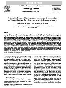
The landing position on each trial may be used to estimate the relative weights attributed to the pre- and post-step velocities, by comparing the observed endpoint with the predicted endpoints based on the two velocities. We then assess how these weights change as a function of time from saccade onset. For instance, if the velocity step occurs long before movement onset the observer will have had more time to base their decision on the post-step, veridical velocity. As will be explained in detail below, fitting these weights over time with a model provides an estimate of the time interval over which object velocity was extracted. Our previous work suggests that the system used a temporal window with a duration of ∼100 ms to estimate target velocity (Etchells, et al., 2010). The end of the window is positioned ∼80 ms before the onset of the saccade. The latter period may be considered the saccadic dead-time, which is functionally defined as the period during which new visual information can no longer affect the saccade endpoint (Becker and Jürgens, 1979; Findlay and Harris, 1984; Aslin and Shea, 1987; Ludwig et al., 2007). The observed endpoint from each trial is converted into a relative weight associated with the post-step velocity. These weights are then fitted with some functional form. Our model is not a process model that specifies the visual mechanisms involved in velocity estimation. However, there is a process interpretation of the model, which is illustrated in Figure 1. We assume that during the latency period object velocity is estimated by convolving the input velocities with some temporal filter (Benton and Curran, 2009) such as that seen in Figure 1. This operation is analogous to computing a running, weighted average of the input. The temporal integration performed by the filter necessarily results in a certain amount of blurring of the velocity information when the velocity is variable. As a result, the observed endpoints may not simply reflect either the pre-step velocity or the post-step velocity, but may be driven by intermediate velocity estimates. The prediction period shown in the figure is assumed to consist of the deadtime and the saccade duration itself. In the present study, our aims were twofold. First, we sought to validate this process interpretation of the model using a straightforward manipulation of the input which is known to profoundly affect the visual system: a variation in contrast. Second, we aimed to simplify the method of fitting the model to make it more

velocity weighng window

Visual info. processing/decision variability

(variable ms)

Dead me ( ~70ms)

Saccade

Saccade end

Target onset

Predicon Period

( ~40ms)

Figure 1 | The time course of a saccade from target detection to the end of the saccade. During this time, average velocity is estimated using a weighting window similar in nature to the one shown here (red solid line). The target is assumed to move at this averaged velocity during the prediction period. This information can then be used to determine where the target is likely to be located at the end of the saccade.

Frontiers in Psychology | Perception Science


Etchells et al.


Alternatively, a reduction in contrast may result in an increase in the time it takes for the incoming velocity information to reach the integration mechanism, as a result of increasing neuronal conduction latencies (e.g., Kaplan and Shapley, 1982). For example, Maunsell et al. (1999) showed that, depending on the number of inputs summed, latency differences in the magnocellular pathway through the lateral geniculate nucleus (LGN) are likely to be on the order of 5–15 ms between high and low intensity stimuli, with high intensity stimuli producing faster responses. A change in the velocity of the lower contrast stimulus will therefore take a longer time to register, which would result in a delay in the velocity signal reaching the integration mechanism. In our methodology, the timeto-peak of the velocity weighting function reflects the time at which emphasis is shifted onto more recent velocity inputs. Therefore, when contrast is reduced, we might expect to see a delay in the point at which a velocity change is detected and incorporated into the final velocity estimate.

Experimental Overview Observers were required to fixate a central diamond-shaped fixation stimulus on a computer screen whilst two Gaussian patches (SD = 0.32°) traversed horizontally across the screen, 6° above and below the midline. During the trial, the fixation point would change into either an upwards- or downwards-pointing arrow, indicating which patch the observers had to make a saccade to (see Figure 2A). On some trials, after a variable delay the speed of the patches would change. By looking at the relationship between saccade landing positions and the time of the speed changes, we can determine how the saccadic system weighs the two velocities over time. We examine the nature of this velocity integration function in two conditions: high and low-contrast. Observers

Six observers were recruited from the students of the University of Bristol, UK (3 females, age range 24–30, mean age 26.0). All had self-reported normal or corrected-to-normal vision. Data B

A

e tim

Figure 2 | (A) Outline of the time course for a rightwards, step up trial. Gaussian patches start moving rightward. After some interval of time the fixation stimulus changes to an arrow, signaling that a saccade to the top patch should be made. After this, the patches step up in speed (illustrated by the double arrows). Note that patches and fixation point are not to scale, for illustration purposes. (B) The fixation stimulus. Removal of either the bottom two or top two diagonal line segments results in an arrow indicating which patch to saccade to.

www.frontiersin.org

were collected over the course of four sessions, performed on different days. The study was approved by the local ethics committee. Eye Movement Recording

Stimuli were displayed on a 21-inch, gamma-corrected CRT monitor (LaCie Electron Blue) running at 75 Hz. The monitor resolution was 1152 × 864 pixels, and the screen subtended 36° × 24° of visual angle. An Eyelink 1000 system (SR Research, Mississauga, ON, Canada) was used to record and monitor eye movements. This is an infrared tracking system that uses the pupil center in conjunction with corneal reflection to sample eye position at 1000 Hz. For each data sample, a dedicated parser algorithm (SR Research, Mississauga, ON, Canada) computes the instantaneous velocity and acceleration of the eye. These are then compared to threshold criteria for velocity (30°/s) and acceleration (8000°/s2). If either is above threshold, the eye movement is classified as a saccade. Visual inspection of a random selection of saccades confirmed that the automatic algorithm placed the on and offsets of the saccades appropriately, without including any apparent contributions from the potential pursuit component that may have followed the saccade. Head position was stabilized at a viewing distance of 57 cm via the use of the Eyelink 1000 built-in chin rest. Observers viewed the display monocularly using their dominant eye, and eye dominance was measured using the hole-in-the-card technique (Seijas et al., 2007). The experimental software was programmed in MATLAB using the Psychophysics Toolbox (Brainard, 1997) and Eyelink Toolbox extensions (Cornelissen et al., 2002). Design and Procedure

Observers performed 28 experimental blocks, each containing 128 trials. Prior to each block, a nine-point calibration procedure was performed in which observers were asked to fixate a black cross that appeared randomly on a 3 × 3 grid. The fixation stimulus measured 0.3° × 0.3°, and the calibration grid subtended 31° × 19° of visual angle. On a given trial, observers were instructed to fixate a central stimulus which took the form of a black diamond containing a cross (see Walker et al., 2000, Experiment 2). Observers were instructed which patch to make a saccade to by the removal of either the top two or bottom two diagonal segments, respectively forming either a downwards or upwards arrow (see Figure 2B). In 50% of the trials within each block, the Gaussian patches would start moving at a constant speed of 18°/s and remain at this speed for the duration of the trial. In 25% of the trials, the patches would step up from 18 to 30°/s at a variable time after the change in fixation stimulus. In the remaining 25% of the trials, the patches would step down to 6°/s. The patches were shown for at least 445 ms before the change in fixation stimulus would occur. After this time, an exponential, i.e., “non-aging,” foreperiod (Nickerson and Burnham, 1969; Oswal et al., 2007) was used to determine the time of the fixation change. A non-aging foreperiod can be described as one in which the probability of a target appearing in the next time interval decreases exponentially over time. This results in an observer’s expectation remaining constant over the course of a trial, which avoids portions of the observer’s response being attributable to something other than the visual information in the stimulus. The mean of this exponential distribution was


Etchells et al.


128 ms. A second non-aging foreperiod, with a mean of 100 ms, was used to determine the time of the speed step. In both cases, a maximum cumulative probability of 95% was used to truncate the distribution, in order to prevent the generation of extremely long foreperiods that would take the patterns off the screen. Within each block the contrast of the patches remained the same, with contrasts being randomized between blocks. Half of the blocks were presented at a high contrast and half at low-contrast. Contrast was defined as Lmax − Lo/Lo where Lo indicates background luminance. This gives contrast values of 80% in the high condition (Lmax = 65.4 cd/m2, Lo = 36.4 cd/m2) and 7.5% in the low condition (Lmax = 39.1 cd/m2, Lo = 36.4 cd/m2).

3 1

X-component landing position error (degrees)

-200

Data analysis

Only data describing the first saccade in each trial were considered. As the minimum distance between the fixation point and target was 6° (when the target was located directly above or below fixation), trials in which the amplitude of the first saccade was less than 4° were rejected, as were trials in which no saccade was generated. Saccade endpoints were recorded, along with the target location at saccade termination and saccade amplitude. The primary analysis concerned the horizontal component of each saccade.

0 -1

200

400

-3 -5

D (ms)

Low contrast

5 3 1

-200

Results For each contrast condition, we first want to determine the extent to which the first orienting saccade is influenced by the pre- and post-step velocities. We do this by measuring, for each trial, the horizontal error between where the saccade landed, and where the target was at the end of the saccade. This saccade endpoint error is then plotted as a function of the time between the velocity step and saccade onset, which we term D. This is aligned on saccade onset, such that D = 0 ms corresponds to the start of the saccade, and D = 500 ms corresponds to the velocity step occurring 500 ms before saccade onset. Figure 3 shows, for a single observer, this landing position error as a function of D for both high and low-contrast conditions. As values of D increase from zero (saccade onset), the general pattern of data in the high contrast condition indicates a gradual increase in the amount of error between the saccade endpoint and the target location at saccade end, up until a time of around 160–170 ms prior to saccade onset. After this time, landing position error decreases back to zero at D = 200–300 ms in the majority of trials. The initial increase in error reflects an over-reliance on the pre-step speed. As D increases, the observers will have seen the target traveling for a longer time at the post-step speed, and therefore will begin to rely more heavily on the veridical velocity. This pattern, whilst similar in the low-contrast condition, shows relatively fewer trials in which the landing position error returns to zero. In those cases where it does, there is an increase in the time it takes for the error to do so, coupled with much greater variability. We now turn to a description of how we estimate the relative weighting of the two velocities, and how these weights can be used to identify the period over which velocity is integrated. For a given observer, we first calculate two errors for each saccade n. εnnew is the difference between saccade landing position and the actual position of the target at the end of the saccade. This error is simply the distance from the zero-error abscissa in Figure 3.


High contrast

5

0 -1

200

400

-3 -5

D (ms)

Figure 3 | D (time between velocity change and saccade onset) versus the x-component error in saccade landing positions for a single observer (observer 1). Data are separated out by contrast condition. Green triangles denote speed step up trials; blue circles denote speed step down trials. Predicted behavior based solely on the post-step speed corresponds to zero-error (i.e., the x-axis). Predicted behavior based solely on the pre-step speed is shown by the red dashed lines.

εnold is the difference between the saccade landing position and the point where the target would have been had it not changed speed. The error that would result from completely following the pre-step velocity is shown by the dashed lines in Figure 3. Note that these predictions depend on the saccade duration and will therefore vary slightly from trial-to-trial. The dashed lines are drawn on the basis of the average saccade duration, just for the purpose of illustration. With these two error terms in place, we determine a relative weighting that the saccadic system places on the post-step velocity, rn, given by: rn =

enold enold − ennew

(1)

Values of rn range between 0 and 1, with rn = 0 equivalent to the saccadic system solely basing its response on the pre-step speed, and rn = 1 equivalent to the system solely utilizing the post-step speed. Figure 4 illustrates (in 15 roughly equal bins) how these weights vary as a function of D. As expected, just before saccade


Etchells et al.


onset, the system has not had time to include the new velocity in its movement program, corresponding to a post-step velocity weight of 0. As time to saccade onset increases, more emphasis is placed on the post-step velocity, eventually reaching values close to 1. It is clear that the transition is gradual, which may be attributed to the varying portions of the pre- and post-step velocities falling under the temporal filter. More formally, if we think of the velocity change as a step function falling within some temporal filter f(t), then rn corresponds to the area under f(t) that falls after the velocity change. Therefore, the plot of rn at a range of values of D gives us the integral of the temporal filter. In order to obtain an estimate of the filter, we fit a reasonable function to these data, and then take its derivative. Note that our actual model fits are based on the data from individual trials, not the binned data which are shown in Figure 4 for illustration purposes only. We opted for maximum likelihood parameter estimation, because this allows us to perform likelihood-based hypothesis testing of the effects of our experimental manipulation on the various properties of the estimated filter (see below; Burnham and Anderson, 2002; Wagenmakers, 2007). Maximum likelihood High contrast 1 0.5

Relative weight attributed to 2nd velocity (ρ)

0 −0.5 −1 0

100

200

300 D (ms)

400

500

Low contrast

1

rn N [r(D),σ(D)]

0.5 0

−0.5 −1 0

requires specification of the probability distribution from which the data points are drawn. This is not straightforward, because it is difficult to know (a) what sources of noise contribute to the variability in the post-step velocity weights and (b) how these noise sources are distributed at any given value for D. In our previous work (Etchells et al., 2010) we assumed that the two types of endpoint error, εold and εnew, were both Gaussian distributed variables. With the weights defined as a ratio, their probability distribution was described as a ratio of Gaussian densities (Marsaglia, 2006). The parameters of the individual Gaussian components depended on a number of variables that were of minor theoretical interest, such as the mean saccade duration, variability in saccade duration, and variability in saccade landing position. An added complication was that these three quantities could, and to some extent did, vary as a function of D. To limit the number of free parameters we used a kernel estimator for the values of these quantities across the entire range of D and incorporated these estimates in the full expression of the probability distribution of r. We appreciate that this procedure is rather cumbersome, for what appears to be a relatively straightforward and lawful pattern of data. We were therefore keen to develop a simplified method and assess to what extent the estimated velocity weights would be affected by the simplification. In the simplified model, we assume that rn is Gaussian distributed, with a mean that varies as a function of D according to some functional form (see below). This is the variation that is of primary theoretical interest. In standard maximum likelihood regression, the SD describes the residuals around the (predicted) mean. It is generally assumed to remain constant and left a free parameter. However, in our case the variability around the (mean) weights clearly varies as a function of D, which can be seen in the size of the error bars in Figure 4. It is important to include this variation: the fit should be most heavily constrained by those data points that were estimated with greater accuracy (i.e., for larger values of D). To make the dependence on D explicit, we write:

100

200

300 D (ms)

400

500

Figure 4 | rn (the relative weight attributed to the post-step velocity) as a function of D (time between velocity change and saccade onset) for a single observer. Dark blue solid line in the top panel denotes the fit of a cumulative Gamma function to the high contrast condition data. Light blue dashed line in the lower panel denotes a Gamma function fit to the low-contrast data. Error bars denote the SD. The dash–dot line in both plots denotes the time at which σn = 0.5, i.e., when both velocities are being weighted equally. Note that while the data are presented here in approximately 15 equal bins, the actual Gamma fit was conducted on the full data set.

www.frontiersin.org

(2)

We were reluctant to introduce additional free parameters to describe the relation between the SD and time from saccade onset. After all, it is not immediately obvious what function best describes this relation and, more importantly, this relation is not of primary theoretical interest. For this reason, we estimated the SD from the observed values of rn using a Gaussian kernel, for values of D ranging from 1 to 500 ms. The bandwidth of this smoothing window was set for each observer separately, to whatever bandwidth best captured the distribution of D sampled for that observer. We reasoned that as the variable of interest is sampled as a function of D, a bandwidth for the optimal sampling of D would provide a reasonable window for smoothing the variability in the weights. Specifically, we computed a weighted SD, for every value of D in 1-ms increments:

r(D )=

∑

N i =1

vi (ri − m(D ))2

∑

N i =1

vi

(3)


Etchells et al.


calculation, as indicated by the more gradual rise to rn = 1 in the low-contrast condition. For clarity, the dash–dot line in Figure 4 illustrates the point at which the two velocities are being weighed equally (i.e., when rn = 0.5), showing a shift from ∼190 to ∼230 ms between the high and low-contrast conditions. Figure 5 shows, for each observer, the derivatives of the weight versus D functions for both contrast conditions. The solid black line shows the filter plot for the high contrast data, and the dashed line shows the filter plot for the low-contrast data. The corresponding shaded regions denote the 95% confidence intervals. These were calculated by producing 1000 bootstrap replications of the fit parameters, using the percentile method (Efron and Tibshirani, 1993). The data show that the filter peaks shift toward larger values of D for the low-contrast condition (M = 207 ms, SEM = 1.5 ms) as compared to the high contrast condition (M = 188 ms, SEM = 2.5 ms), for every single observer. There also appears to be a slight increase in the width of the filter as contrast is reduced (M = 79 ms, SEM = 6.7 ms in the high contrast condition, M = 88 ms, SEM = 7.7 ms in the low-contrast condition). These effects are not concomitant with an increase in saccade latency in the step conditions – in the high contrast condition, the mean saccade latency across all observers was 271 ms (SEM = 8.3 ms), compared to a mean saccade latency of 274 ms (SEM = 6.5 ms) in the low-contrast condition – an increase of only 3 ms. The

Here the vector of weights, ω, is the Gaussian smoothing function sampled at 1-ms intervals and μ is the Gaussian-weighted mean. To capture r(D) we initially chose a scaled cumulative Gamma function. The Gamma function was chosen to accommodate both symmetric and asymmetrical filters, and has frequently been used to describe temporal filters (Watson, 1986; Smith, 1995). The smooth curves in Figure 4 show the fits of the simplified model. These curves are characterized by three free parameters, namely a (the upper asymptote – the lower bound was set to zero), k (shape), and θ (scale). The Nelder–Mead Simplex method (Nelder and Mead, 1965) was used in order to find the set of best-fitting parameters. It is clear that these functions describe the data well. For each of the 12 data sets reported in the paper (six observers and two contrast levels), we computed the correlation between the predicted weights estimated using the original and simplified fitting methods, for the observed values of D. In all cases the correlation was greater than 0.99. As such, the drastically simplified model results in very similar velocity weighting functions as the more complete (and complex) model developed in our previous work. Having established the viability of the simplified model, we now turn to the empirical question of interest: what is the effect of contrast on the velocity weighting function? For the data shown in Figure 4, it appears that it takes the system much longer to incorporate the post-step speed into the saccade landing position

Normalised Weighting (arbitrary units)

2.0

2.0

P1

1.5

1.5

1.0

1.0

0.5

0.5

0 0 2.0

100

200

300

400

500

P2

0 0 2.0

1.5

1.5

1.0

1.0

0.5

0.5

0 0 2.0

100

200

300

400

500

P3

0 0 2.0

1.5

1.5

1.0

1.0

0.5

0.5

0 0

100

200

300

400

500

D (ms)

0 0

P4

100

200

300

400

500

P5

100

200

300

400

500

P6

100

200

300

400

500

D (ms)

Figure 5 | Velocity integration filters for all six observers in Experiment 1. Solid dark blue line denotes the plot based on the high contrast data; dashed light blue line denotes the plot for the low-contrast data. Shaded areas indicate 95% confidence limits based on 10,000 bootstrap replications (dark blue and light green for high and low-contrast conditions, respectively).



Etchells et al.

s accade latency should correspond to any changes in the saccadic go signal (i.e., the fixation stimulus change). However, if as a result of the reduction in contrast, it is harder to localize the target (for example, for the purposes of the final position grab), then we might reasonably expect that the saccade latency would increase. The fact that we do not see this is important, as it shows that peak shifts that we see are not simply a result of “stretching” that occurs due to a general increase in the time it takes to detect or generate a saccade to a lower contrast target. To assess the effects of contrast more formally, we adopted a model selection approach (Burnham and Anderson, 2002; Wagenmakers, 2007). Indeed, this was the motivation for estimating the model parameters using maximum likelihood. For this purpose, we defined a number of competing models that represent different hypotheses about the effect(s) of contrast. The likelihoods of these models constitute an index of the amount of evidence provided by the data for the different hypotheses. The following four competing models were defined. If contrast had no effect on the width or peak location of the filter, we would expect a set of four parameters to suffice – a single peak location parameters, a width parameter, and two separate asymptotes (this is hereafter known as the baseline model). At the other extreme, contrast could affect every possible aspect of the filter, necessitating two separate sets of three parameters to account for the data. We refer to this model as the saturated model. In between these two extremes fall two reduced models of critical interest: (1) a fiveparameter peak location model accommodates the data from both contrast conditions with a common width, but allows the location and asymptote to vary with contrast; (2) a five-parameter width model which assumes different widths and asymptotes for the low and high contrasts. In other words, we force the location and/or widths to be the same. One problem with the Gamma function is that its parameters do not correspond to experimentally interesting parameters such as filter width and peak position. This makes it very difficult to, for example, test the competing models that we have outlined above. Therefore, for the purpose of this test, we chose to fit our data with scaled cumulative Gaussian curves, instead of the Gamma functions used earlier. As can be seen in Figure 5, the identified temporal filters are relatively symmetrical. Seeing as this is the case, a Gaussian function is attractive because its two parameters are independent and correspond directly to the location and width parameters of the filter. In comparison, the shape and scale parameters of the Gamma interact to jointly determine its location and width. The inability of the Gaussian to accommodate the slight asymmetries in the filters, did result in a decreased goodness-of-fit, as we will show below. However, the critical components of the filter, the width and location, were numerically very close under both models. Moreover, the effect(s) of contrast on these two components was also very similar when estimated with Gaussian or Gamma functions. For this reason, we see the reduction in goodness-of-fit as a price worth paying for the greater utility of the Gaussian function in terms of parameter interpretation. Finally, the four models defined above differ in the number of free parameters. In evaluating their likelihoods, it is desirable to take this variation in complexity into account. A Bayesian information criterion (BIC) adjusts the log-likelihood of a model, given

www.frontiersin.org


the observed data and best-fitting parameters, according to the number of free parameters (Schwarz, 1978; Wagenmakers, 2007). In particular: BIC= − 2L + k ln(N )

(4)

where L is the maximum log-likelihood, k is the number of free parameters of a model, and N is the number of observed data points. As is readily apparent from Eq. 4, the BIC balances goodness-of-fit with parsimony. Models with smaller BICs are more competitive, as those with a greater number of free parameters (which should produce a better fit) are penalized. Table 1 shows the values of the BICs for all four models and observers, the summed totals across the sample, as well as the BICs for the fits of the saturated Gamma functions for each observer. The Gamma function is the clear overall winner with the lowest BIC – the BIC difference with the saturated Gaussian model is 41, which corresponds to a corrected likelihood-ratio, or Bayes factor, of greater than 1000 (Wagenmakers, 2007). Thus it is clear that fitting the data with a Gaussian function results in a less desirable fit of the data; however, the Gaussian still offers a considerable advantage in terms of the interpretability of the parameters. Moreover, inspection of a plot of the weightings based on the best-fitting Gaussian and Gamma (both full and simplified versions) models shows that all three functions fit the data reasonably well (see Figure 6). With respect to the Gaussian model comparisons then, the fiveparameter location model is the winning model by a clear margin. In other words, allowing a peak shift, but not a width shift, provides the best description of the data. The BIC difference with the nearest competitor – the saturated Gaussian model – is ∼37, which again corresponds to a Bayes factor, of greater than 1000. The direct comparison between the width and location models also came out strongly in favor of the location model (a combined BIC difference of almost 100). In both circumstances, the size of the Bayes factor corresponds to an effective p value of