Testing and implementation of an improved water quality index for ...

Summary Report

Testing and implementation of an improved water quality index for the 2016 and 2017 Great Barrier Reef Report Cards Summary Report Cedric Robillot, Murray Logan, Mark Baird, Jane Waterhouse, Katherine Martin and Britta Schaffelke

Testing and implementation of an improved water quality index for the 2016 and 2017 Great Barrier Reef Report Cards SUMMARY REPORT Cedric Robillot5, Murray Logan1, Mark Baird2, Jane Waterhouse3, Katherine Martin4, Britta Schaffelke1 Australian Institute of Marine Science 2 CSIRO Oceans and Atmosphere 3 School of Marine and Tropical Biology, James Cook University 4 Great Barrier Reef Marine Park Authority 5 eReefs, Great Barrier Reef Foundation 1

Supported by the Australian Government’s National Environmental Science Program Project 3.2.5 Testing and implementation of an improved water quality index for the 2016 and 2017 Great Barrier Reef Report Cards

© Australian Institute of Marine Science, 2018

Creative Commons Attribution Testing and implementation of an improved water quality index for the 2016 and 2017 Great Barrier Reef Report Cards: Summary Report is licensed by the Australian Institute of Marine Science for use under a Creative Commons Attribution 4.0 Australia licence. For licence conditions see: https://creativecommons.org/licenses/by/4.0/ National Library of Australia Cataloguing-in-Publication entry: 978-1-925514-19-3 This report should be cited as: Robillot, C., Logan, M., Baird, M., Waterhouse J., Martin, K. and Schaffelke, B. (2018) Testing and implementation of an improved water quality index for the 2016 and 2017 Great Barrier Reef Report Cards: Summary Report. Report to the National Environmental Science Program. Reef and Rainforest Research Centre Limited, Cairns (65pp.). Published by the Reef and Rainforest Research Centre on behalf of the Australian Government’s National Environmental Science Program (NESP) Tropical Water Quality (TWQ) Hub. The Tropical Water Quality Hub is part of the Australian Government’s National Environmental Science Program and is administered by the Reef and Rainforest Research Centre Limited (RRRC). The NESP TWQ Hub addresses water quality and coastal management in the World Heritage listed Great Barrier Reef, its catchments and other tropical waters, through the generation and transfer of world-class research and shared knowledge. This publication is copyright. The Copyright Act 1968 permits fair dealing for study, research, information or educational purposes subject to inclusion of a sufficient acknowledgement of the source. The views and opinions expressed in this publication are those of the authors and do not necessarily reflect those of the Australian Government. While reasonable effort has been made to ensure that the contents of this publication are factually correct, the Commonwealth does not accept responsibility for the accuracy or completeness of the contents, and shall not be liable for any loss or damage that may be occasioned directly or indirectly through the use of, or reliance on, the contents of this publication. Cover photographs: Gary Cranitch; MODIS - NASA This report is available for download from the NESP Tropical Water Quality Hub website: http://www.nesptropical.edu.au

Testing and implementation of an improved water quality index

TABLE OF CONTENTS List of Tables ......................................................................................................................... iii List of Figures........................................................................................................................ iv Acronyms .............................................................................................................................. vi Glossary ............................................................................................................................... vii Acknowledgements ............................................................................................................. viii Executive summary ............................................................................................................... 1 1.0 Summary of project approach .......................................................................................... 6 2.0 Assimilation of surface reflectance observations into the eReefs BGC ............................ 8 2.1 Principles and Methods ................................................................................................ 8 2.2 Results and model performance .................................................................................10 3.0 Data sources ..................................................................................................................12 3.1 AIMS in situ sampling .................................................................................................12 3.2 AIMS logger data ........................................................................................................13 3.3 Satellite remote sensing data ......................................................................................13 3.4 Non-assimilating eReefs BGC model (eReefs926)......................................................16 3.5 eReefs BGC model with assimilation of remote-sensing reflectance (eReefs) ............16 4.0 Water quality threshold values and key metric parameters .............................................17 4.1 Reporting time period ..................................................................................................17 4.2 Spatial domains for reporting ......................................................................................18 4.3 Indicators ....................................................................................................................19 4.4 Water quality threshold values ....................................................................................21 5.0 Exploratory data analysis and fitness for purpose ...........................................................24 5.1 Annual data.................................................................................................................24 5.2 Spatial data .................................................................................................................28 5.3 Comparison of data sources .......................................................................................30 6.0 Index calculations ...........................................................................................................37 6.1 Theoretical framework ................................................................................................37 6.2 Index sensitivity ..........................................................................................................42 7.0 Aggregation hierarchies and scoring ..............................................................................45 8.0 Reef Report Card 2016 ..................................................................................................47 8.1 Revised water quality metric Report Card outputs.......................................................47 8.2 Analysis of differences between the original and revised marine water quality metric .50 8.2.1 Source data ..........................................................................................................53 8.2.2 Properties of individual reporting sites ..................................................................54 i

Robillot et al

8.2.3 Index scoring method ...........................................................................................54 8.2.4 Temporal aggregation strategy .............................................................................55 8.2.5 Reporting year definition .......................................................................................56 8.2.6 Reporting zone boundaries...................................................................................56 8.2.7 Summary of comparison findings for Chlorophyll-a ...............................................57 9.0 Conclusion and future improvements .............................................................................59 9.1 Project outcomes and recommendations ....................................................................59 9.2 Future improvements ..................................................................................................60 References ...........................................................................................................................63

ii


LIST OF TABLES Table 1:

Table 2: Table 3: Table 4:

Table 5: Table 6:

Overview of chlorophyll-a data sources available for the metric along their relative characteristics. The shading of the various cells reflects a subjective assessment of how well each method performs against each characteristic. . 12 Example of water quality measure hierarchy specifying which measures contribute to which indicators......................................................................... 21 Water quality threshold values for selected key measures ............................. 23 Formulations and example response curves for a variety of indicator scoring methods that compare observed values (xi) to associated benchmark, thresholds or references values (Bi and dashed line). The Scaled Modified Amplitude Method can be viewed as three Steps: I. Initial Score generation, II. Score capping (two alternatives are provided) and III. Scaling to the range [0,1]. A schematic within the table illustrates the different combinations of Modified Amplitude formulations. The first of the alternative capping formulations simply caps the Scores to set values (on a log2 scale), whereas the second formulation (Quantile based, where Q1 and Q2 are quantiles) allows threshold quantiles to be used for capping purposes. Dotted lines represent capping boundaries. In the Logistic Scaled Amplitude method, T is a tuning parameter that controls the logistic rate (steepness at the inflection point). For the purpose of example, the benchmark was set to 50. .............................................................................. 40 Index performance and sensitivity data scenarios .......................................... 42 Summary of the effect of discrete changes to the calculation method to derive the metric and comparison with the resulting overall differences between the original and revised metric scores for Chlorophyll-a ....................................... 58

iii

Robillot et al

LIST OF FIGURES Figure 1:

Figure 2: Figure 3: Figure 4: Figure 5:

Figure 6: Figure 7: Figure 8:


Figure 12:

Figure 13: Figure 14:

Figure 15:

Figure 16:

Figure 17:

iv

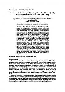
Overview of the revised water quality metric generation process for Report Card 2016. (* Measure standardised to Indices on a continuous scale of 0 (very poor) to 100 (very good) by expressing individual values relative to corresponding thresholds according to a modified amplitude indexation routine (base 2 logarithm of the ratio of observed value to threshold) ....................................... 5 Overview of the metric calculation strategies ................................................... 6 Schematic showing eReefs coupled hydrodynamic biogeochemical model ..... 8 Schematic showing the evolution of the model ensemble over 6 assimilation cycles using the Ensemble Kalman Filter (EnKF) system ................................ 9 Comparison of the non-assimilating (blue) and assimilating (pink) eReefs BGC runs at MMP sites. The instantaneous state root mean square error is represented at the 14 MMP sites (top). At Double Cone Island in the Whitsundays (off Airlie Beach), a time-series of the observations (black dots) and simulations is shown for the whole simulation period (centre) and a one year period (bottom) ...................................................................................... 11 Map of AIMS in situ MMP sites (left) and spatial and temporal distribution (right - blue shading of tiles denote the number of surveys conducted in the year). 14 Spatial and temporal distribution of AIMS FLNTU data (Red: turbidity. Green: chlorophyll-a fluorescence). ........................................................................... 15 Townsville daily accumulated rainfall for October 1st 2016 to February 13th 2017. Also shown are the daily median (1942 to present) rainfall as well as the five previous years. .............................................................................................. 17 GBR reporting zones as combinations of NRM regions and water bodies ..... 19 TSS to turbidity ratio based on MMP data (from Waterhouse et al., 2017) ..... 22 Observed (logarithmic axis with violin plot overlay) TSS data for the Wet Tropics Open Coastal Zone from a) AIMS in situ, b) AIMS FLNTU loggers, c) Satellite and d) eReefs (assimilating) .......................................................................... 25 Observed (logarithmic axis with violin plot overlay) chlorophyll-a data for the Wet Tropics Open Coastal Zone from a) AIMS in situ, b) AIMS FLNTU loggers, c) Satellite and d) eReefs (assimilating) ............................................................. 27 Spatial distribution of observed a) AIMS in situ, b) satellite, c) eReefs and d) eReefs926 Chlorophyll-a for the Burdekin Midshelf Zone .............................. 29 Location of satellite data grid cells within 5km of AIMS in situ sampling sites. Panel borders represent water bodies (Red: Enclosed Coastal, Green: Open Coastal, Blue: Midshelf) ................................................................................. 32 Location of eReefs data grid cells within 5km of AIMS in situ sampling sites. Panel borders represent water bodies (Red: Enclosed Coastal, Green: Open Coastal, Blue: Midshelf) ................................................................................. 33 Temporal patterns in chlorophyll-a within 5km of each AIMS MMP sampling site for eReefs, satellite and AIMS in situ and FLNTU logger sources. Horizontal dashed line represents the threshold value. Title backgrounds represent water bodies (Red: Enclosed Coastal, Green: Open Coastal, Blue: Midshelf). ........ 35 Simulated data and associated indices for threshold of 0.1 and large sample sizes (R=1000) .............................................................................................. 43


Figure 18: Figure 19: Figure 20: Figure 21:


Figure 25: Figure 26:

Figure 27:

Figure 28:

Figure 29:

Simulated data and associated indices for threshold of 100 and large sample sizes (R=1000) .............................................................................................. 43 Temporal, measure and spatial aggregation hierarchy .................................. 45 Score to grade conversion charts. In each case, the scale along the base defines the grade boundaries ........................................................................ 46 Overview of the revised water quality metric generation process for Report Card 2016. (* Measure standardised to Indices on a continuous scale of 0 (very poor) to 100 (very good) by expressing individual values relative to corresponding thresholds according to a modified amplitude indexation routine (base 2 logarithm of the ratio of observed value to threshold) ..................................... 48 Simplified (Zone mean) eReefs spatio-temporal fsMAMP chlorophyll-a and Secchi depth index grades (Uniform score to grade conversion applied) ....... 49 Extract from Reef Report Card 2016 showing the water quality metric results at the regional and whole-of-GBR level ............................................................. 50 Comparison of the new WQ metric (eReefs with data assimilation, represented by circles and continuous lines) against the previous WQ metric (remote sensing, represented by squares and dashed lines) for overlapping years 201314 and 2014-15. Note that the previous WQ metric was not reported for the Cape York and Burnett Mary regions because of limited confidence in the remote sensing-based estimates in these regions. ........................................ 51 Overview of the original water quality metric generation process for Report Card 2015 (original metric). .................................................................................... 52 Comparison of Chlorophyll-a scores when using the eReefs BGC (solid line) or remote sensing (dashed line) data in the revised (top) or original metric (bottom) calculations. For comparison purposes the enclosed coastal data was not included in either metric calculations. ............................................................ 54 Comparison of Chlorophyll-a scores when using the binary compliance (solid line) or fsMAMP (dashed line) index scoring using as source data the eReefs BGC (top) or remote sensing (bottom). For comparison purposes the temporal aggregation strategy is the same, with daily index calculations subsequently aggregated over the entire water year. .......................................................... 55 Comparison of Chlorophyll-a scores when using the binary compliance index scoring method, calculated daily with subsequent aggregation over the water year (solid line) or calculated based on the annual mean of Chlorophyll-a concentration (dashed line). The source data used is the eReefs BGC (top) or remote sensing (bottom). ............................................................................... 55 Dry Tropics region. Original marine water quality metric score for Chlorophyll-a and TSS for inshore waters with enclosed coastal waters included and excluded. Annual discharge and annual sediment loads. Source: Roger Shaw using data from Dieter Tracey, DNRM and Bureau of Meteorology. ............... 56

v

Robillot et al

ACRONYMS AIMS ............. Australian Institute of Marine Science BOM.............. Bureau of Meteorology CSIRO........... Commonwealth Scientific and Industrial Research Organisation DERM ........... Department of Environment and Resource Management EECs ............. Essential Ecosystem Characteristics FU ................. Functional Unit GBR .............. Great Barrier Reef GBRF ............ Great Barrier Reef Foundation GBRMP ......... Great Barrier Reef Marine Park GBRMPA ...... Great Barrier Reef Marine Park Authority IMOS ............. Integrated Marine Observing System ISP ................ Independent Science Panel JCU ............... James Cook University MMP.............. Marine Monitoring Program MODIS .......... Moderate Resolution Imaging Spectroradiometer NAP .............. Non-algal particulates NESP ............ National Environmental Science Program P2R ............... Paddock 2 Reef RRRC............ Reef and Rainforest Research Centre Limited TSS ............... Total Suspended Solids TWQ.............. Tropical Water Quality WQIP ............ Water Quality Improvement Plan

vi


GLOSSARY AIMS FLNTU

Data from continuous deployments of Combination Fluorometer and Turbidity Sensors (WET Labs Environmental Characterization Optics (ECO) FLNTUSB (Fluorescence, NTU) loggers), collected by AIMS as part of the MMP

AIMS In situ

Data from analysis of direct water samples (collected manually, using Niskin bottles) collected by AIMS as part of the MMP

Chlorophylla

The green pigment found in cyanobacteria, algae and plants. Chlorophyll-a concentration is widely used as a proxy for phytoplankton biomass as a measure of the productivity of marine systems, eutrophication status and to indicate nutrient availability

eReefs BGC

eReefs biogeochemical model of the Great Barrier Reef as described in http://ereefs.info

Indicator

An overall characteristic of interest, e.g. water quality

Index

Standardized representation of a measure typically expressed relative to a benchmark, guideline or threshold

Measure

A numerical value of an environmental response that has been measured (directly in field) or obtained by calculation from other measures.

Metric

Mathematical formulation or expression used to generate an index

MMP

Marine Monitoring Program

NOx

Dissolved oxidised nitrogen, the sum of nitrate and nitrite

NTU

Nephelometric Turbidity Units

Region

Natural Resource Management (NRM) Region

Satellite

Data derived from Bureau of Meteorology MODIS satellite imagery

Secchi Depth The depth at which a 8-inch (20cm) disk of alternating white and black quadrants is no longer visible from the surface of fluid Subindicator

A major component of interest of the Indicator, a grouping of a set of measures, e.g. Water Clarity

TSS

Total Suspended Solids, a measure for the concentration of particulate matter in the water. A measure of light scattering caused mainly by suspended solids, algae, microorganisms and other particulate matter, conventionally measured using a sensor (nephelometer) as Nephelometric Turbidity Units (NTU). One of the five water bodies as defined by the Great Barrier Reef Marine Park Authority in GBRMPA (2010)

Turbidity

Water Body Zone

Combination of Region and Water Body

vii

Robillot et al

ACKNOWLEDGEMENTS We thank Peter Doherty, Roger Shaw, Hugh Yorkston, Carl Mitchell and the Reef 2050 Water Quality Improvement Plan Independent Science Panel for their scientific advice. We thank Carol Honchin and Bronwyn Houlden from the Great Barrier Reef Marine Park Authority for guidance on marine water quality guidelines and boundaries of water bodies. We thank Eric Lawrey from the Australian Institute of Marine Science for assistance with the management of data on eAtlas. We thank Emlyn Jones, Jennifer Skerratt, Nugzar Margvelashvili, Farhan Rizwi and Mike Herzfeld from CSIRO for the implementation of the eReefs models and data assimilation scheme. The eReefs Project is a collaboration between the Great Barrier Reef Foundation, Bureau of Meteorology, Commonwealth Scientific and Industrial Research Organisation, Australian Institute of Marine Science and the Queensland Government, supported by funding from the Australian Government’s Caring for our Country, the Queensland Government, the BHP Billiton Mitsubishi Alliance, and the Science Industry Endowment Fund. Atmosphericallycorrected MODIS products were sourced from the Integrated Marine Observing System (IMOS) - IMOS is supported by the Australian Government through the National Collaborative Research Infrastructure Strategy and the Super Science Initiative.” This research was supported by the Australian Government’s National Environmental Science Program Tropical Water Quality Hub, administered in North Queensland by the Reef and Rainforest Research Centre Ltd, and by the Great Barrier Reef Marine Park Authority.

viii


EXECUTIVE SUMMARY Introduction The Reef 2050 Water Quality Improvement Plan (Reef Plan) guides how industry, government and the community will work together to improve the quality of water flowing into the Great Barrier Reef (GBR). Foundational to the water quality theme of Reef 2050 Long-term Sustainability Plan, the Reef Plan is a joint commitment of the Australian and Queensland governments to address all land-based run-off flowing from the catchments adjacent to the GBR. The plan sets the strategic priorities for the whole Reef catchment. Regional Water Quality Improvement Plans, developed by regional natural resource management bodies, support the Reef Plan in providing locally relevant information and guiding local priority actions within regions. The annual Great Barrier Reef Report Card (Report Card), which is integrating the information from a range of programs monitoring and modelling land management practices, pollutant levels and the condition of the GBR and its catchments, is the main mechanism to evaluate progress towards targets and identify whether further measures need to be taken to address water quality in the GBR. In previous Report Cards (until 2015), marine water quality was reported using a metric based on satellite remote sensing of near surface concentrations of chlorophyll and total suspended solids, which provided a wide spatial and temporal coverage of marine water quality which cannot be achieved with in situ observations. Index scores for these indicators were calculated based on the relative area of the inshore water body that did or did not exceed the relevant GBRMPA Water Quality Guidelines (GBRMPA 2010). Scores for Chl-a and NAP were aggregated (averaged) into a final metric value subsequently converted into a final grade on a five-point uniform scale (translated into grading statements: very good, good, moderate, poor, very poor) for each Natural Resource Management (NRM) Region . This final grade describes the overall water quality condition across the GBR and within each individual NRM Region. Complementing the Report Card metric, the results of in situ monitoring of water quality have been reported annually to provide detailed, site-specific information on temporal trends and spatial patterns1. The water quality metric used underpinning previous Report Cards (until 2015) presented a number of significant shortcomings: • It was solely based on remote sensing-derived data. Concerns were raised about the appropriateness of exclusively relying on remote sensing to evaluate inshore water quality, considering well-documented challenges in obtaining accurate estimates from optically complex waters and the fact that only limited valid satellite observations are available in the wet season due to cloud cover; • It was limited to reporting on two indicators and did not incorporate other water quality data and indicators collected through the Marine Monitoring Program (MMP) and the Integrated Marine Observing System (IMOS); • It appeared relatively insensitive to large terrestrial inputs into the GBR lagoon during large rainfall and runoff events, most likely due to the binary assessment of compliance See 2016 summary report: http://www.reefplan.qld.gov.au/measuring-success/report-cards/2016/assets/report-card-2016detailed-results.pdf and the detailed reports from the Marine Monitoring Program available at: http://elibrary.gbrmpa.gov.au/jspui/browse?type=series&order=ASC&rpp=20&value=Marine+Monitoring+Program++Inshore+Water+Quality 1

1

Robillot et al

relative to the water quality guidelines and aggregation and averaging over large spatial and temporal scales; In 2016, based on the limitations described above, the Reef Plan Independent Science Panel (ISP) expressed a lack of confidence in the water quality metric that underpinned Report Cards (prior to 2015) and recommended that a new approach be identified for the Report Card 2016 and future Report Cards. The ISP also acknowledged substantial advancements in modelling water quality through the eReefs biogeochemical models and the fact that recent research and method development2 had improved our ability to construct report card metrics. To address the above shortcomings, the ISP requested that: • The e-Reefs marine biogeochemical (BGC) model be tested for its ability to deliver a better water quality assessment than the current practice based on remote sensing; • The GBRMPA water quality guidelines be reviewed to incorporate new evidence collected over the last 6-8 years in understanding coral and seagrass responses to chronic and acute pressures, ecosystem health, recovery and resilience; • The utility of observational data streams from in-situ monitoring is analysed for potential inclusion in Report Card; • The current practice of scoring relative to water quality guidelines and aggregating data over fixed spatial and temporal scales be improved to incorporate the magnitude, frequency and duration of exceedance rather than simply using average annual exceedance counts; • The inclusion of photic depth, as derived from satellite data, into the metric be evaluated since light is the important driver for coral and seagrass productivity. The most appropriate measure of photic depth can be evaluated and related to seagrass and coral responses; and • Options for combining indicator scores into a single metric are evaluated, including a statistical assessment of potential metrics. These recommendations were the basis for formulating this NESP 3.2.5 project entitled “Testing and implementation of an improved water quality index for the 2016 and 2017 Great Barrier Reef Report Cards”. Conducted as a collaboration between GBRMPA, AIMS, CSIRO and JCU, the high-level objective for this project were to identify, investigate and assess alternative strategies to integrate available monitoring and modelling data into an improved water quality metric for the GBR marine waters. An additional set of objectives was to identify, in consultation with key stakeholders, how preliminary findings could be incorporated into Report Card 2016 and to provide recommendations for further improvements to the metric in subsequent report cards. To achieve these objectives and meet the timelines of Report Card 2016, significant improvements had to be demonstrated by April 2017. Project outcomes and recommendations • The systematic analysis and comparison of different sources of water quality data (in situ water sampling, continuous fluorescence loggers, eReefs BGC model and satellite

Such as a Reef Rescue-funded project on data integration (Brando et al. 2013) and data aggregation methods developed for and used in the recent Gladstone Healthy Harbour Partnership report card 2

2


data) available to derive a water quality metric did not lead to a recommendation to exclude any specific source of information; •

An innovative data assimilation scheme was developed to assimilate satellite reflectance information into the eReefs BGC model. Extensive validation and model skill assessment was conducted to demonstrate the performance of the assimilating model, including individual time series comparisons and absolute and normalised error statistics across all observation locations.

•

Strategies to integrate these data sources were developed and evaluated. Approaches based on the direct aggregation of independent data sources were shown to be deficient due to the radically different spatial and temporal distributions of the data. The preferred approach was to assimilate satellite reflectance information into the eReefs BGC model and to rely on in situ measurements for validation of the model performance.

•

Index scoring strategies were systematically assessed to meet key objectives of sensitivity and representativeness, to allow data aggregation and to enable the integration of additional water quality measures when these become available in the future. A preferred method was identified as the scaled modified amplitude method with fixed caps sets at half and twice the threshold values, which was tested both theoretically and using historical datasets.

•

Aggregation strategies were reviewed and a hierarchical aggregation scheme was developed to allow multiple measures and sub-indicators to be combined into a single metric and to allow spatial and temporal aggregation. The process was designed to maintain the richness of information and allow the propagation of uncertainty, which were key project objectives.

•

The resulting water quality metric calculation process and parameters were applied to the development of the marine water quality metric component of Reef Report Card 2016, covering the reporting period 1 October 2015 to 30 September 2016.

•

Opportunities for future research and improvement were identified during the course of the project and are detailed in section 0.

Project governance and independent scientific oversight As discussed in the introduction, the genesis of this project was in recognition that a new approach was needed to report marine water quality for Report Card 2016 and future Report Cards. Therefore, the project scope was to a large extent prescribed by Report Card stakeholders (Queensland and Australian Governments, GBRMPA) with its delivery conducted under the direct scientific oversight of the Reef Plan Independent Science Panel (ISP). The project sought guidance and input from the ISP and GBRMPA for parameters driving the metric simulations, when no clear scientific recommendation could be established for the selection of these parameters or when the review of such parameters was out of scope. Technical elements forming an integral part of the broader Report Card framework and which could not be altered without leading to reporting inconsistencies were considered out of scope for this project. Examples included spatial reporting boundaries, guidelines, score-to-grade conversion scales and colour schemes.

3

Robillot et al

The project reported at ISP meetings on more than five occasions and obtained endorsement from ISP for all key parameters, including: • Temporal reporting boundaries, with the reporting period based on the same water year definition as the AIMS MMP (Waterhouse et al., 2017), starting on 1 October of the previous calendar year and finishing on 30 September of the same calendar year; •

Spatial reporting boundaries, based on the combinations of six NRM regions (Cape York, Wet Tropics, Burdekin3, Mackay Whitsunday, Fitzroy and Burnett Mary) and four water bodies (Enclosed Coastal, Open Coastal, Midshelf and Offshore);

•

Threshold values based on existing marine water quality guidelines for the following water quality measures: concentration of chlorophyll-a, dissolved oxidised nitrogen (NOx) and total suspended solids (TSS) (equivalent to non-algal particulate (NAP)) and Secchi depth;

•

Identification of two sub-indicators to underpin the water quality metric as chlorophylla concentration (productivity sub-indicator) and Secchi depth (water clarity subindicator). The confidence in modelled data and associated threshold values for TSS and NOx was not considered sufficient to include these measures in the final metric; and

•

Score to grade conversion scale (uniform scale), which is used to translate the water quality metric scores into a Report Card grade and colour (from very good to very bad).

Revised Water Quality metric for Report Card 2016 The project successfully delivered an improved marine water quality metric for Report Card 2016, now incorporating results from all six NRM regions. Results can be found at http://www.reefplan.qld.gov.au/measuring-success/report-cards/2016/ and the process for generation of the metric outputs is summarised in Figure 1. The results obtained with the new metric were compared to those generated using the original metric because understanding how changes to the source data and metric calculation process impacted final reporting outputs was considered essential in terms of maintaining stakeholder confidence in the overall marine water quality reporting framework. The only common sub-indicator between the two metric versions is Chlorophyll-a. Significant differences between the original and revised metric for Chlorophyll-a were observed in the Burdekin and Wet Tropics regions, with the revised metric generating much higher Chlorophylla scores, which can be interpreted as better water quality. Such differences led to a similar improvement in the Reef-wide Chlorophyll-a score and also the regional and Reef-wide overall water quality scores. A systematic analysis of the factors that led to such differences confirmed the source data as the main factor, specifically the switch from remote sensing extraction of water quality data to the eReefs BGC model with data assimilation. This is not unexpected considering the premise for this project was to address confidence issues in relation to the water quality data extracted 3

4

The terms Burdekin and Dry Tropics are used interchangeably throughout the reports to define this NRM Region


from remote sensing. These improvements in both source data and index calculation method have led to an increased confidence in the metric results, as indicated by a better representation of North-South and cross-shelf gradients that are represented in and known to exist from actual observational data.

Figure 1: Overview of the revised water quality metric generation process for Report Card 2016. (* Measure standardised to Indices on a continuous scale of 0 (very poor) to 100 (very good) by expressing individual values relative to corresponding thresholds according to a modified amplitude indexation routine (base 2 logarithm of the ratio of observed value to threshold)

5

Robillot et al

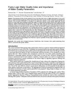
1.0 SUMMARY OF PROJECT APPROACH This project was articulated around a number of discrete and to a large extent independent tasks which are listed below. This Summary Report contains a section for each of these tasks. • Developing a new eReefs biogeochemical model simulation based on the assimilation of remote sensing reflectance data and validating the outputs of the simulation over several reporting years through a skill assessment against independent in-situ observations (such as in situ sampling and loggers) (Section 1.0) • Identifying, processing and comparing the various sources of monitoring and modelling data (including the new eReefs simulation) and assessing their fitness for the purpose of calculating a revised metric (Sections 3.0 and 5.0); • Establishing metric parameters such as water quality thresholds based on existing guidelines, temporal and spatial domains for aggregations and suitable indicators (Section 4.0); • Investigating metric calculation strategies including the generation of water quality measures and indices as well as aggregation and scoring strategies (Sections 6.0 and 7.0); • Engaging with Reef Plan ISP to reach consensus on a preferred metric calculation approach for Report Card 2016 and generating outputs for incorporation into said report card (Section 8.0); and • Identifying areas for future improvements to the metric and associated research and development needs (Section 9.0). Figure 2 provides a conceptual summary of two clearly distinct data processing and metric calculation strategies as these were envisaged at project inception, based on either: • Calculating index scores for various indicators based on individual independent data sources such as in situ sampling, remote sensing and eReefs BGC modelling; or • Assimilating remote sensing reflectance information into the eReefs BGC model and calculating index scores for various indicators based on the outputs of the dataassimilated eReefs BGC model.

Figure 2: Overview of the metric calculation strategies

Figure 2 highlights the fact that investigations and findings into the calculation of indices, aggregation and scoring will be common to different data streams provided the data is

6


processed adequately, which justifies the mostly independent nature of these investigations. In this summary and in the main report, these different components are treated independently.

7

Robillot et al

2.0 ASSIMILATION OF SURFACE REFLECTANCE OBSERVATIONS INTO THE EREEFS BGC This component of the project is described in detail in section 2.5 of the main report.

2.1 Principles and Methods The eReefs coupled hydrodynamic, sediment and BGC modelling system involves the application of a range of physical, chemical and biological process descriptions to quantify the rate of change of physical and biological variables (Figure 3, Schiller et al. (2014)). Details on the modelling framework and relevant reports and publications can be found on the http://ereefs.info website and further information is provided in section 2.5.1 of the main project report.

Figure 3: Schematic showing eReefs coupled hydrodynamic biogeochemical model

The processes descriptions are generally based either on a fundamental understanding of the process (such as the effect of gravity on circulation) or measurements when the process is isolated (such as the maximum division rate of phytoplankton cells at 25°C in a laboratory monoculture). The model also requires as inputs external forcings, such as observed river flows and pollutant loads. Thus, the model can be run without observations from the marine environment and in this mode is quite skilful (Skerratt et al. (in revision)). This mode which does not use observations from the marine environment as the simulation is undertaken is referred to as the non-assimilating simulation. Most of the eReefs marine biogeochemical simulations are non-assimilating.

8


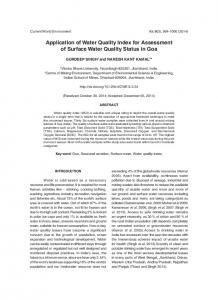
Despite being already skilful, the predictive skill of the model can be improved by assimilating marine observations into an ensemble (i.e. a large number (108) of similar but not identical) of model simulations. The form of data assimilation chosen within this project, and that is commonly used in weather forecasting, involves updating of the state of the model as the simulation progresses as described in Figure 4 and summarised below.

Figure 4: Schematic showing the evolution of the model ensemble over 6 assimilation cycles using the Ensemble Kalman Filter (EnKF) system

The non-assimilating control run (black line) is capturing the gross cycle in the observations (blue stars), but errors remain that observations can constrain. The process steps are described below: • At the initial time, all ensemble members, and the control run, have similar values. In the first five days the 108 members develop a spread, with the control run being different to the ensemble mean, but within the ensemble spread. • At 5 days, the first state updating occurs. In the first 5 days there was only one observation, being above the ensemble mean. At day 5, a new state for the entire ensemble is calculated (the analysis being the mean of the updated ensemble) based on the mismatch between the ensemble members and observations. The updated state is closer to the model if the ensemble spread is small, or to the observations if they are dense with few errors. At day 5, because of the small positive mismatch, the ensemble spread is only slightly narrowed, and the mean increased. The ensemble members all restart from these new updated states. • The next four analysis steps proceed much like the first. For the fifth analysis step, high density observations were available over the previous 5 days, so the analysis is weighted heavily toward the observations, and the model spread is constrained significantly. Looking at the error between the ensemble mean and the observations over the entire period the data assimilation system has provided an improved estimate of the state (the mean of the ensemble) relative to the control run and achieved this using the model that contains the processes we understand to describe the system. 9

Robillot et al

In the case of the eReefs BGC, ocean colour, the observation of water-leaving irradiance at 8 individual wavebands, provides the only data set with sufficient temporal (daily) and spatial (1 km) resolution, providing upwards of 13 million pixels on a cloud-free day. This comparison relies on the mismatch between the model’s prediction of the ratio of the water-leaving irradiance at 443 nm (blue) and 551 nm (green) and the observation of the same quantities from the MODIS sensor on NASA’s Aqua satellite. The eReefs BGC model is the first published model to assimilate raw ocean colour observations (Jones et al., 2016). The data assimilation algorithm uses the model-observation mismatch, as well as statistically-quantified dynamical properties of model, to periodically alter the values in the 108 member ensemble, resulting the ensemble mean gaining a closer match to the observations. The outcome of this modelling system is referred to in the field of data assimilation as a reanalysis.

2.2 Results and model performance In our assessment of the skill of the eReefs biogeochemical models, we have considered the most important property to be the prediction of in situ chlorophyll concentration at the existing MMP water quality monitoring sites. For this there are two measures – the chlorophyll-a concentration data from standard analyses by extraction of chlorophyll-a from water samples, and the calibrated chlorophyll fluorescence data from deployed instruments (see Waterhouse et al. 2017 for sampling methods). While the chlorophyll-a concentrations derived from water sample analyses are considered the most accurate, the fluorescence time-series is continuous. When the two are lined up in time, the root mean square difference between the observed chlorophyll-a concentrations from water sample analyses and the observed chlorophyll fluorescence is on average 0.2 mg m-3. This is a relatively small error for fluorescence measurements and we use 0.2 mg m-3as indicative of the error of the fluorescence time series. The non-assimilating version of the model has been compared to observations previously (http://ereefs.info, Baird et al. (2016) and Skerratt et al. (in revision)). The results produced in the reanalysis are compared directly to observations in a detailed report appendix showing comparisons to hundreds of time-series. Further components of this document compare the metric calculated using the non-assimilating model, the assimilating model, satellite observations and in situ observations. In this summary and in the main report, only a few snapshot results are presented to aid in the understanding of the performance of the data assimilation relative to the non-assimilating run. It is important to note that no in situ chlorophyll concentration observations were assimilated into the model. That is, they were observations withheld just for the model assessment. In fact, the mismatch between observed and modelled quantities used in the assimilation system is neither an in situ measurement, nor a chlorophyll concentration. The assimilated quantity was the ratio of remote-sensing reflectance at blue and green wavelengths. Thus, we can be confident that if the assimilation system has improved the prediction of in situ chlorophyll concentration then it has improved the overall biogeochemical model. At 13 of the 14 MMP sites, the assimilation of satellite-observed remote-sensing reflectance improved the prediction in situ chlorophyll concentration (Figure 5, top). On average the assimilation reduced the error from 0.34 to 0.29 mg m-3, bringing it 30 % closer to the 10


observation error (the limit of our ability to quantify an improvement in the model). The worst two sites remained the most coastal sites, Geoffrey Bay and Dunk Island, for which the 4 km model poorly resolves local processes, and for which the assimilation system would provide little information to the water column due to the optically-shallow and complex waters. The best site was Double Cone Island off Airlie Beach. At this site, a time-series shows the improvement in the chlorophyll fluorescence due to the assimilation (Figure 5, bottom). During a particularly cloud-free period in the second half of 2015, the assimilation system performs remarkably well at both removing model bias and capturing variability in the model.

Figure 5: Comparison of the non-assimilating (blue) and assimilating (pink) eReefs BGC runs at MMP sites. The instantaneous state root mean square error is represented at the 14 MMP sites (top). At Double Cone Island in the Whitsundays (off Airlie Beach), a time-series of the observations (black dots) and simulations is shown for the whole simulation period (centre) and a one year period (bottom)

11

Robillot et al

3.0 DATA SOURCES This component of the project is described in detail in sections 2.2 to 2.6 of the main report. Data sources to be used for a metric need to meet a range of conditions which has led to the selection of a limited number of sources. These conditions include: • Availability and continuity of the data over multiple years, allowing trend analysis; • Standard (accepted) techniques; • Quality controlled and/or validated measures with an estimate of intrinsic uncertainty; • Adequate spatial and temporal distribution. Considering the vast GBR domain, it is unlikely that any data source would meet all required conditions fully and compromises have to be considered when selecting data for inclusion in the metric (see example in Table 1). As an example, it is generally accepted that in situ measurements of chlorophyll-a (grab sample and laboratory measurement method) are the most accurate however these are infrequent and represent only a limited number of discrete sites (as opposed to the entire domain). Extraction of chlorophyll-a properties from satellite surface reflectance data is generally considered to present a lower relative accuracy however the method covers a much wider spatial domain on a daily basis (when not affected by cloud cover). For the purpose of the metric, five sources of data were considered (AIMS in situ and logger measurements, satellite data, non-assimilating and assimilating eReefs BGC) which are discussed further below. Table 1: Overview of chlorophyll-a data sources available for the metric along their relative characteristics. The shading of the various cells reflects a subjective assessment of how well each method performs against each characteristic.

Method

Continuity (# years available)

Accuracy (certainty)

Temporal distribution (frequency)

Spatial distribution (coverage)

Comments

AIMS in situ AIMS loggers Satellite (MODIS)

Affected by cloud cover

eReefs

Only available since late 2010

3.1 AIMS in situ sampling The AIMS component of MMP inshore water quality monitoring sampling program has been designed to quantify spatial and temporal patterns in inshore water quality, particularly in the context of catchment loads. Details of the sampling design and methods are in Waterhouse et al., 2017. From 2006–2014, AIMS visited 20 sites, three times per year (roughly corresponding to wet, early and late dry seasons), see Figure 6. The sites were largely selected along approximate north-south transects proximal to major rivers so as to provide samples along an expected water quality gradient (exposure to runoff). Following a review in 2014, the design was modified to intensify the spatial (32 sites) and temporal (typically between 5 and 10 samples per year) coverage of the sampling program. In particular additional sampling effort was applied around three priority focal areas (Russell-Mulgrave, Tully and Burdekin).

12


Parameters measured that are of relevance to this project include turbidity, Secchi depth, concentrations of chlorophyll-a, dissolved oxidised nitrogen (NOx) and total suspended solids (TSS) (equivalent to non-algal particulate (NAP)).

3.2 AIMS logger data Combination Fluorometer and Turbidity Sensors (WET Labs Environmental Characterization Optics (ECO) FLNTUSB (Fluorescence, NTU) loggers), referred to herein as FLNTU loggers, were continuously deployed at 15 of the AIMS MMP inshore water quality monitoring sites (Figure 7) and provide data on chlorophyll concentration (measured as chlorophyll fluorescence, in µg L-1 or mg m-3) and turbidity (expressed in nephelometric turbidity units, NTU).

3.3 Satellite remote sensing data Satellites provide time series from November 2002 to present of surface reflectance (ocean colour) with spatial coverage at 1 km resolution for the whole-of-GBR lagoon, nominally on a daily basis. Coastal waters are optically complex and global algorithms have been found to be of limited use. CSIRO have developed regionally validated algorithms that incorporate the regional and seasonal knowledge of optical properties of GBR waters. The ocean colour dataset consists of processed satellite imagery, currently from the MODIS Aqua satellite and in the future from the VIIRS satellite (eReefs Phase 2). The image processing uses multiple algorithms developed by NASA, the CSIRO and other agencies and is now housed at the Bureau of Meteorology's National Meteorological and Oceanographic Centre (NMOC) under the Marine Water Quality Dashboard (http://www.bom.gov.au/marinewaterquality/). The data referred to herein relates to the individual measures considered in the data exploration component of the project, what is commonly referred to as specific inherent optical properties, and is distinct from the surface reflectance data used in the eReefs data assimilation scheme as discussed previously. There measures include non-algal particulate concentrations, Secchi depth and chlorophyll-a concentration. Daily (July 2002–Dec 2016, 1km x 1km resolution) imagery data were obtained by downloading NETCDF files from the Bureau of Meteorology’s Thredds server4.

4

http://ereeftds.bom.gov.au/ereefs/tds/catalog/ereef/mwq/P1D/2002/catalog.html

13

Robillot et al

Figure 6: Map of AIMS in situ MMP sites (left) and spatial and temporal distribution (right - blue shading of tiles denote the number of surveys conducted in the year).

14


Figure 7: Spatial and temporal distribution of AIMS FLNTU data (Red: turbidity. Green: chlorophyll-a fluorescence).

15

Robillot et al

3.4 Non-assimilating eReefs BGC model (eReefs926) As mentioned in Section 0, the eReefs coupled hydrodynamic, sediment and BGC modelling system involves the application of a range of physical, chemical and biological process descriptions to quantify the rate of change of physical and biological variables (Figure 3, Schiller et al. (2014)). Details on the modelling framework and relevant reports and publications can be found on the http://ereefs.info website and further information is provided in section 2.5.1 of the main project report. The eReefs BGC model gbr4_bgc_926, is referred to as eReefs926 in this project, has a resolution of 4km x 4km and outputs are delivered on an hourly basis for a large number of water quality variables, including the following parameters of relevance to this project: chlorophyll-a, non-algal particulate (EFI proxy), Secchi depth calculated from light attenuation at 490 nm and NOx as NO3 concentration. Detailed technical reports and validation results (updated in January 2017) can be found at https://research.csiro.au/ereefs/models/.

3.5 eReefs BGC model with assimilation of remote-sensing reflectance (eReefs) The reflectance data assimilation scheme is discussed in detail in section 0. The eReefs BGC model with assimilation (reanalysis) is referred to as eReefs in this report, has a resolution of 4km x 4km and provides outputs on a daily basis from 2013 to 2015 for the same suite of variables as the non-assimilating eReefs BGC model.

16


4.0 WATER QUALITY THRESHOLD VALUES AND KEY METRIC PARAMETERS A number of key parameters had to be considered in the initial phase of the project as these were expected to impact the metric simulations significantly and required endorsement from external stakeholders. These include temporal and spatial reporting boundaries and reference values for various water quality measures and are discussed in more detail below.

4.1 Reporting time period Report cards are typically compiled and communicated annually. However, the time window that constitutes a year differs from report card to report card. Many environmental report cards communicate on data collected within a financial year which provides a reporting window that is consistent with other management considerations. Others use a time window that naturally aligns with the cycle of some major underlying environmental gradient - such as wet/dry season. For this project, the same water year definition as the AIMS MMP (Waterhouse et al., 2017) was adopted which starts on 1 October of the previous calendar year and finishes on 30 September of the same calendar year. To illustrate this approach, the Reef Report Card 2016 water quality metric would be reporting on data collected between 1 October 2015 and 30 September 2016. This approach was endorsed by Reef Plan ISP. The main factor taken into consideration when deciding on the reporting period was to ensure that the data collected would capture the key processes expected to impact water quality in the GBR lagoon, in this case the significant river discharges which take place with increased rainfall in the wet season. Seasonal aggregation (wet versus dry period) is not considered appropriate at this stage as the start of such periods may vary significantly year to year and basin to basin, and there is no current agreed method to address this variability in a metric. Figure 8 below shows that a 1 October start is likely to capture the start of the wet season (based on rainfall) which is a critical factor.

Figure 8: Townsville daily accumulated rainfall for October 1st 2016 to February 13th 2017. Also shown are the daily median (1942 to present) rainfall as well as the five previous years. 17

Robillot et al

4.2 Spatial domains for reporting The Great Barrier Reef Marine Park (GBR), spans nearly 14° of latitude, covers approximately 344,400km2 and in so doing spans multiple jurisdictions with differing pressures and management strategies. Furthermore, the GBR also spans a substantial longitudinal range being bounded by the Queensland coastline in the west and the outer reef in the east. Hence, it is useful to partition the GBR into smaller more homogeneous zones representing combinations of region and water body. This project relied on boundaries already accepted by managers and decision makers on the GBR, namely the combinations of six NRM regions (Cape York, Wet Tropics, Burdekin, Mackay Whitsunday, Fitzroy and Burnett Mary) and four water bodies (Enclosed Coastal, Open Coastal, Midshelf and Offshore), as per Figure 9. Following recommendations of the Reef Plan ISP, the Enclosed Coastal zone is excluded from the majority of high level metric simulation products, reflecting limitations of the eReefs 4km resolution model in dealing with small coastal areas and issues associated with the representativeness of the Enclosed Coastal Zone boundaries considering the significant variations in annual river discharge. Nevertheless, it has been retained in part of the exploratory data analysis for information purposes as well as to provide some validation and justification for the proposed approach.

18


Figure 9: GBR reporting zones as combinations of NRM regions and water bodies

4.3 Indicators One of the biggest challenges of report card development is the selection of appropriate indicators from amongst a potentially very large candidate pool. Since the outcomes, conclusions and implications are all dependent on the indicators selected, the selection process is one of the most influential steps and has justifiably received a great deal of attention. As part of their ecosystem report card framework, Harwell et al. (1999) urged that the alignment of scientific information with societal goals and objectives should be the guiding principle of indicator selection. In their framework, clearly articulated societal goals and objectives (a combination of societal values and scientific knowledge, such as restored and sustainable wetland system) are translated into Essential Ecosystem Characteristics that represent a set of generic attributes that further refine the broad goals (such as water quality, sediment quality, 19

Robillot et al

habitat quality, ecological processes). The characteristics are then further translated into a set of scientific informed indicators that are measured or monitored to indicate the status of trends or states associated with these characteristics. There have since been numerous studies that have focused on providing more formal, objective criterion for indicator selection. Whilst the specifics vary, most can be broadly encapsulated by Dauvin et al. (2008) and their contextual implementation of the Doran (1981)’s SMART (Simple, Measurable, Achievable, Realistic, and Time limited) principle. A ’good’ indicator should be representative, easily interpreted, broadly comparable, sensitive to change and have a reference or guideline value. To be ‘useful’, an indicator must be approved by international consensus, be well grounded and documented, have a reasonable cost/benefit ratio and have adequate historical and on-going spatial-temporal coverage. Since final outcomes are likely to be highly influenced by indicator choice, the robustness and sensitivity of both indicators and final outcomes to changes in ecosystem health should be understood if not formally investigated as part of the indicator selection process (Dobbie and Dail, 2013). Sensitivity analyses can involve: • simulating changes in the underlying data of different magnitudes and estimating the resulting sensitivity (percentage or probability of change) expressed by the indicator; or • estimating the effect of past perturbations on the indicator hindcasted from historical data As stressed above, indicators should align intimately with report card objectives. Yet in the broader ecosystem report card frameworks, such indicators are often too general to be measurable. Therefore, in such cases, the indicators are further sub-divided into progressively more specific measures. For example, an indicator of water quality might comprise subindicators of nutrients, metals and physico-chemistry which in turn might be represented by more specific measures such as total nitrogen, mercury, dissolved oxygen, pH etc. The resulting design is a hierarchical structure in which sub-indicators (etc) are nested within indicators and spatial scales are nested from entire regions, sub-regions or zones down to individual sites or sampling units. One of the strengths of such a hierarchical report card framework is that the inherent inbuilt redundancy allows for the addition, deletion or exchange of finer scale items (sites and actual measured variables) with minimum disruption to the actual report indicators. That is, the indicator is relatively robust to some degree of internal makeup. Furthermore, by abstracting away the fine details of an indicator, similar indicators from different report cards (each potentially comprising different sampling designs) are more directly comparable. For example, in different report cards that include water quality, a water quality indicator of ’water clarity’ might comprise different Measures (e.g. suspended solids, NTU, Secchi depth etc) collected from different sources (e.g. satellite, in situ loggers or hand samples), yet provided each of these water clarity indicators are well calibrated, it should be possible to compare state and trend across the report cards. In the context of Reef Report Card, the objective is primarily to report on the water quality condition of the GBR lagoon ecosystem. Such condition is impacted by a number of factors, such as river discharge and transport of contaminants, cyclonic activity and resuspension of sediments, upwelling events and others. Both natural processes (rainfall, ocean circulation and extreme weather events) and anthropogenic activities (land management practices, coastal 20


development and industrial activities) may influence these factors however a condition-based metric is not in principle designed to differentiate between these influences. Therefore, the notion of metric sensitivity needs to be understood as the responsiveness of the metric to the overarching factors, as opposed to a direct response to some of the underpinning influences. A typical example is the impact of river discharge on coastal water quality. While land management practices in the catchment have a direct impact on contaminant loads discharged by various rivers, the most significant impact on coastal water quality condition is expected to be the annual amount of rainfall, with water quality decreasing significantly during wet years such as experienced in 2011. An appropriate metric would therefore be expected to be generally responsive to said annual rainfall level. In terms of indicators, the scope of this project is limited to considering and assessing indicators that are accepted and for which adequate data is available at this point in time. However it is acknowledged that a number of independent initiatives are currently considering issues related to water quality indicators, most notably the development of the Reef 2050 Integrated Monitoring and Modelling Program (RIMMReP) yet also various NESP projects researching the development of light-related indicators. Therefore, the design of a revised metric needs to be flexible to seamlessly integrate new indicators in the future. The nested approach described above and the index calculation and aggregation methods proposed in this project achieve this objective. Key indicators of water quality condition that were considered for further investigation in this project are productivity, nutrients and water clarity. Potential measures contributing to these indicators for which adequate data may be available include chlorophyll-a, NAP (TSS), turbidity, Secchi depth and NOx (example in Table 2). Other indicators and or contributing measures were not considered practical or justifiable based on the limited monitoring data available or the lack of relevant guidelines. Table 2: Example of water quality measure hierarchy specifying which measures contribute to which indicators

Indicator

Sub-indicator

Measure

Productivity

Chlorophyll-a NAP (TSS)

Water Quality

Water clarity

Turbidity Secchi depth

Nutrients

NOx

4.4 Water quality threshold values An environmental health metric represents the state or condition relative to some reference, threshold or expectation. Most of the current water quality indices compare values to a set of specifically selected guidelines. These guidelines are either formulated specifically from longterm historical data appropriate to the spatial and temporal domain of interest or else are based 21

Robillot et al

on ANZEC guidelines (Australian and New Zealand Environment and Conservation Council, 2000). There are some clear principles as to how, and in which circumstances, such guidelines should be applied. As an example, marine water quality guidelines for chlorophyll-a in the GBR lagoon should be applied to annually aggregated data - not individual observations – as these guidelines are based on a predicted ecological outcome based on annual averages. Since this project intends to generate indices on the scale of individual observations, we have decided to define reference values as threshold values to avoid contradicting principles for the implementation of guidelines. In reporting zones where a GBRMPA water quality guideline is available, this is used as the threshold value. This is the case for all TSS (NAP), chlorophyll-a and Secchi depth threshold values in Open Coastal, Mid-shelf and Offshore water bodies. In reporting zones where a GBRMPA water quality guideline is not available, i.e. for enclosed coastal waters, Queensland water quality guidelines are systematically used unless a site-specific or region-specific value could be identified. No guideline value is currently available for the measure turbidity in Open Coastal, Mid-shelf and Offshore waters. Threshold values were set by considering a simplified linear relationship between TSS values and turbidity based on the large MMP data set, leading to a ratio of approximately 1.3 as per Figure 10. It is not suggested that this overly simplistic relationship can be used to extrapolate turbidity from TSS or vice versa.

Figure 10: TSS to turbidity ratio based on MMP data (from Waterhouse et al., 2017)

The threshold values identified for each Measure within each Water body are indicated in

22


Table 3. These apply to all regions equally, are based on existing guidelines where possible and were endorsed by Reef Plan ISP. Whilst the application of seasonal thresholds could potentially remove some uncertainty, in the absence of clear consensus on how to define wet and dry seasons and what the associated set of reference values would be, seasonal threshold values are not used in this project.

23

Robillot et al

Table 3: Water quality threshold values for selected key measures

Water body Measure

Unit

Chlorophylla

µg.L-

NAP (TSS)

Turbidity Secchi Depth

24

Open Coastal

Midshelf

Offshore

0.45

0.45

0.4

1

2

2

0.7

NTU

1.5

1.5

1

m

10

10

17

1

mg.L-

Comments GBRMPA WQ guidelines used as threshold values GBRMPA WQ guidelines used as threshold values No guideline available, application of calculated turbidity threshold value based on relationship between TSS and turbidity as per MMP (see above) GBRMPA WQ guidelines used as threshold values


5.0 EXPLORATORY DATA ANALYSIS AND FITNESS FOR PURPOSE This component of the project is described in detail in section 3 of the main report. Exploratory data analysis is vital for informing data processing and analysis as well as establishing assumptions and limitations. Of particular importance for the current project is the spatial and temporal distribution and variability of the various data measures and sources as these impact how data can be compared and aggregated and how various indices and scores may be calculated.

5.1 Annual data Using all available data for each measure, exploratory plots were generated to visualise the data distribution in relation to threshold values as mentioned in section 0. These plots can be found in appendix to the main report however examples are discussed below to illustrate principles and key findings. Figure 11 presents a typical analysis for TSS in the Wet Tropics Open Coastal zone based on four different data sources: AIMS in situ water sampling, turbidity data from FLNTU loggers converted to TSS, remote sensing (NAP) and eReefs modelled data (assimilating mode). Observations are presented over time and coloured conditional on season as Wet (blue symbols) and Dry (red symbols). The blue smoothed line represents the product of a Generalized Additive Mixed Model within a water year and the purple straight line represents the average within the water year. Horizontal red, black and green dashed lines denote the twice threshold, threshold and half threshold values, respectively. Red and green background shading indicates the range (10% shade: x4,/4; 30% shade: x2,/2) above and below threshold respectively. Such information-rich plotting approach provides significant context and facilitates the qualitative comparison of independent data sources which is a challenging aspect considering the diversity of monitoring approaches in terms of spatial and temporal distribution.

25

Robillot et al

Figure 11: Observed (logarithmic axis with violin plot overlay) TSS data for the Wet Tropics Open Coastal Zone from a) AIMS in situ, b) AIMS FLNTU loggers, c) Satellite and d) eReefs (assimilating)

All of the figures are presented with log-transformed y-axes as the data are typically positively skewed. This is expected for parameters that have a natural minimum (zero), yet no theoretical maximum. It does however mean that these distributional properties should be considered during the analyses. In particular, for mean based aggregations, outliers and skewed distributions can impart unrepresentative influence on outcomes. Each of the data sources present different variability characteristics. The scale of the range of AIMS in situ data is predominantly and approximately less than or equal to the scale of the half/twice the associated threshold value. The AIMS FLNTU logger data have a larger range than the AIMS in situ data - presumably because the former data collection frequency captures most of the peaks and troughs whereas the latter are unlikely to do so. Furthermore, whilst the

26


AIMS in situ data are predominantly collected during the dry season, the AIMS FLNTU loggers collect data across the entire year and are therefore likely to record a greater proportion of the full variation in conditions. Of course it is important when interpreting these diagnostic plots to focus mainly on the violin plots and less on the dots (representing individual observations). This is because the dots do not provide an indication of the density and it is easy to allow outliers to distort out impression of the variability of the data. Similarly, the scale of the range of eReefs data is approximately equal to the scale of the range of the span from half/twice the threshold value. This reflects both a more complete time series and broader spatial extent represented in the data. In contrast to the AIMS in situ and to a lesser extent the AIMS FLNTU and eReefs data, the scale of the range of the satellite data is relatively large - typically a greater span than the range of half/twice threshold value. Figure 12 presents a similar analysis for chlorophyll-a in the same zone. Analyses have been conducted for all reporting zones (region x water body) and proposed measures and are available in the main report. Monthly analyses (as opposed to annual) can also be found in the report. The exploration of the temporal distribution of various data sources does not justify excluding any particular data set from the metric simulations. While some variability between monitoring or modelling methods is evident, no systematic bias or significant anomaly is observed which would disqualify a specific data source.

27

Robillot et al

Figure 12: Observed (logarithmic axis with violin plot overlay) chlorophyll-a data for the Wet Tropics Open Coastal Zone from a) AIMS in situ, b) AIMS FLNTU loggers, c) Satellite and d) eReefs (assimilating)

28


5.2 Spatial data The spatio-temporal patterns in observed data were explored and an example for the Burdekin Midshelf Zone is provided in Figure 13. Colour scales have been mapped to a constant value range for each source for a given Measure, the lower and upper bounds of which are based on the minimum and maximum data range for the Measure within the Region/Water body combination across all years. These figures highlight the disparity in resolution between the different data sources. The AIMS in situ data is spatially very sparse and in fact the logger data, being even sparser, was not represented. The satellite data has the most extensive spatial resolution and notwithstanding the many gaps due to various optical interferences (such as cloud cover), also has the greatest temporal coverage. For the selected Zones and span of water years, there is little evidence of a major latitudinal gradient in satellite chlorophyll-a with most of any change (if any) occurring across the shelf. Indeed, the satellite parameters are relatively constant over space and time for the Burdekin Midshelf Zone. Moreover, the spatial patterns of satellite-derived Chlorophyll-a and TSS appear relatively invariant between years. The eReefs and eReefs926 data do show some variability in spatial and temporal chlorophylla and Secchi depth yet relatively little for TSS and NOx (at least for Burdekin Midshelf). Whilst this apparent lack of variability is largely an artefact of the colour scale mapping, the values of these Measures are constantly substantially below the threshold value and thus invariant on the scale considered appropriate for comparison against the associated thresholds. The entire set of spatial distribution analysis plots can be found in the eReefs online repository (https://eatlas.org.au/nesp-twq-3/3-2-5-analysis-catalogue). In this case again, and even though the satellite data seems to show very limited responsiveness in time and space, there is not enough evidence to justify excluding a specific data set. The fact that the in situ sampling data, which could be considered a reference, is so sparse also contributes to a conservative approach with regard to the potential exclusion of data.

29

Robillot et al

Figure 13: Spatial distribution of observed a) AIMS in situ, b) satellite, c) eReefs and d) eReefs926 Chlorophyll-a for the Burdekin Midshelf Zone

30


5.3 Comparison of data sources Ensuring that the data underpinning the metric calculations are suitable for this purpose is a critical part of the process, especially if multiple data sources for a specific indicator are to be aggregated as part of these calculations. For example, successful aggregation of chlorophylla as modelled by the eReefs BGC with chlorophyll-a as extracted from satellite reflectance data (optical properties) will largely depend on the underlying compatibility of these two sources. Moreover, further combining with far more sparse and irregular sources (such as AIMS in situ chlorophyll-a samples) relies on general patterns of spatial and temporal autocorrelation being present across the denser data sources so as to facilitate a projection of sparse data across the denser layers. The five different sources (AIMS in situ, AIMS FLNTU loggers, satellite, eReefs and eReefs926) were all collected at different spatio-temporal resolutions. Specifically: • the Satellite data are collected on a 1km grid on a daily basis, however there are many gaps in the time series of each cell due to cloud cover and other issues that affect the reliability of observations; • the eReefs data are modelled and projected on to a 4km grid on a daily basis without any time series gaps between 2013 and 2016; • the eReefs926 data are modelled and projected on to a 4km grid on a daily basis without any time series gaps between 2011 and 2014; • the AIMS in situ samples are collected from specific sampling sites (28-32 throughout the GBR) and on an infrequent basis (approx. 3-4 times per year although more frequently in later years). Furthermore, apart from relatively recently, the majority of samples were collected in the dry season and thus these samples could be biased towards long term water quality trends rather than short-term pulses. • the AIMS FLNTU logger data are deployed at a subset (16) of the AIMS in situ sampling locations and record measurements every 10 minutes (although there are frequent gaps due to instrument failure). The AIMS in situ sampling locations are strategically positioned to generally represent transects away from major rivers discharging into the GBR. As such, they likely represent biased estimates of the water parameters of the surrounding water bodies. Nevertheless, the observed data are direct measurements of a range of parameters considered to be important measures of water quality and are therefore considered to be relatively accurate estimates of the true state - albeit for a potentially narrow (and biased) spatio-temporal window. By contrast, the satellite data represent indirect proxies for some of these parameters (chlorophyll-a, TSS and Secchi depth) and similarly, the eReefs data are indirect modelled estimates simulated from a deterministic implementation of a conceptual model. Hence, to gauge the accuracy of the satellite and eReefs data (and thus inform qualitative confidence), time series and spatial patterns in the Satellite and eReefs observations were compared to the AIMS in situ observations. The disparate spatio-temporal resolutions of the data sources present substantial challenges for extracting comparable data. For example, the proximity of AIMS in situ samples to reefs and the spatial resolution (1km or 4km grid) frequently result in an inability to obtain matching 31

Robillot et al

spatial location for all three sources, especially in shallow waters where both the satellite and eReefs data present significant limitations. Furthermore, gaps in the satellite time series frequently prevent matching satellite data to the same day as AIMS in situ sampling. Compounding these issues is the added inherent complications and ‘noise’ associated with the inability to control exactly when sampling occurs throughout dynamic environments. For example, in situ samples are collected (date as well as time of day) based largely on logistics whereas the availability of acceptable satellite data is determined by when the satellite passes over the GBR and whether the data are of sufficient quality. The degree to which the discrete AIMS in situ samples reflect space and time around the actual sampling sites/times is largely unknown. That is, it is not clear how broadly representative the direct observations are. Consequently, it is difficult to estimate how broadly to filter the satellite and eReefs data in space and time around the AIMS in situ sampling sites/events in order to generate comparable data. The ’best’ breadth is likely to be a compromise between data availability (time limited for satellite and space limited for eReefs) and data equivalence (the degree to which samples from different sources are considered to represent the same spatiotemporal unit). Figure 14 and Figure 15 illustrate the spatial distribution of satellite and eReefs grid cell centroid locations relative to the AIMS in situ sampling locations. The different colour spokes denote distance categories (red:

Testing and implementation of an improved water quality index for ...

Testing and implementation of an improved water quality index for ...

Suggest Documents