it can be seen in Baddeley and Van Lieshout (1995) and Dasgupta and Raftery ... Murchison data set, that has been widely used by Adrian Baddeley in many of ...
Testing covariate significance in spatial point process first-order intensity M.I. Borrajo, W. Gonz´alez-Manteiga and M.D. Mart´ınez-Miranda Abstract Modelling the first-order intensity function in one of the main aims in point process theory, and it has been approached so far from different perspectives. One appealing model describes the intensity as a function of a spatial covariate. In the recent literature, estimation theory and several applications have been developed assuming this hypothesis, but without formally checking the goodness-of-fit of the model. In this paper we address this problem and test whether the model is appropriate. We propose a test statistic based on a L2 -distance; we prove the asymptotic normality of the statistic and suggest a bootstrap procedure to calibrate the test. We present two applications with real data and a simulation study to better understand the performance of our proposals.
1
Introduction
The understanding of the spatial distribution of point patterns is crucial in many different fields: ecology (Illian et al. (2009) and Law et al. (2009)); epidemiology (Lawson (2013)); seismology (Ogata and Zhuang (2006) and Schoenberg (2011)); forestry (Stoyan and Penttinen (2000)); geology (Foxall and Baddeley (2002)); and also plays an important role in statistical theory, see for example Daley and Vere-Jones (1988),Diggle (2013) and Cressie (2015). Initially, from the point of view of statistical inference, the main interest of spatial point process theory was to test the complete spatial randomness (CSR) hypothesis, i.e., to determine if a pattern come from a homogeneous Poisson process, in which case the underlying intensity is constant over the observation region; distance-based and quadrat counts are the classical methods on this topic, see Diggle (2013) and Cressie (2015) for more detail. Moreover, some applications have been developed under this assumption, as it can be seen in Baddeley and Van Lieshout (1995) and Dasgupta and Raftery (1998). The first order characteristics, among which the intensity function is the most important one, have been also studied from different perspectives, and it is formally defined as: E[N (dx)] λ(x) = lim , |dx|→0 |dx| 1
where N is the counting measure, i.e., N is the random variable that counts the number of points lying on a given set. Assumed parametric models and using for instance a likelihood score, see Van Lieshout (2000), Moller and Waagepetersen (2003) and Diggle (2013) or pseudolikelihood procedures, see Waagepetersen (2007) may generate unreliable estimates when it deviates from the true one. Hence the nonparametric approach is a well-known alternative. Diggle (1985) proposed the first kernel intensity estimator which has been widely used in exploratory analysis. The main disadvantage of this estimator is its lack of consistency, for which Cucala (2006) proposed a modification based on the relationship between the intensity and the density functions. Recently, this lack of consistency and some real applications requirements induced a new scenario based on the inclusion of covariates in the model. Guan (2008) proposed a kernel intensity estimator, assuming that the intensity function depends on some observed spatially varying covariates through an unknown continuous function. The consistency of his estimator was proved under an increasing domain asymptotic framework, and he also deals with the problem of high dimensional covariates. Later, Baddeley et al. (2012) considered spatial covariates postulating that λ(x) = ρ(Z(x)), x ∈ W ⊂ R2 ,
(1)
where Z : W ⊂ R2 → R is a spatial continuous covariate that is exactly known in every point of the region of interest W . Their proposal includes some intensity estimators based on the local likelihood as well as some kernel estimators, but without proper theoretical developments. Borrajo et al. (2017) have developed in detail the theoretical properties of a kernel intensity estimator in this context of point processes with covariates; proposing a specifically designed bootstrap procedure and data-driven bandwidth selectors. The inclusion of spatially varying covariates has been a big step forward on point process theory; however, a little attention has been paid to test the significance of these covariates. To the extent of our knowledge, only something similar has been done in a slightly different context in D´ıaz-Avalos et al. (2014), where the authors assume that the intensity depends on a linear combination of several covariates and they test, using the conditional intensity function, if any of the coefficients may be null. In this work we try to fulfil the existing gap on checking the goodness-of-fit of model (1) by defining a new testing procedure. This paper is organised as follows. Section 2 is devoted to present in detail the two motivating examples we use all along the manuscript. In Section 3 the statistical test is introduced, detailing its asymptotic null distribution and a bootstrap procedure which is used to improve its calibration. The methodology proposed is applied to the real data sets in Section 4. The performance of the test is analysed in Section 5 through a simulation study based on real data analyses in order to make it more realistic. Finally we draw some remarks in Section 6.
2
2
Motivating examples
In this section we motivate our proposal using two real data set. The first one is the Murchison data set, that has been widely used by Adrian Baddeley in many of his papers, books and software; and a new data set made up of wildfires in Canada.
Figure 1: Murchison geological survey data; gold deposits (points) and geological faults (lines). The Murchison geological survey data shown in Figure 1 record the spatial locations of gold deposits (a total number of 255) and the surrounding geological faults. These data came from a 330 × 394 km region in the Murchison area of Western Australia and have been obtained from Watkins and Hickman (1990). At this scale (1:500000) the gold deposits spatial extension is negligible and they can be considered as points without losing generality. Note that the real gold deposits and faults are three-dimensional while here we use a two-dimensional projection. Moreover, some geological faults may have been missed because they are not recorded by direct observation but in magnetic field surveys or geologically inferred from discontinuities in the rock sequences. Once we have the locations of the gold deposits and the faults, the construction of the covariate is simple, we have to compute the distance from every point in the observation region to the nearest fault (see Figure 2). We use this covariate to model the intensity of the process following (1).
3
Figure 2: Covariate information for the Murchison data set: distance to the nearest geological fault (in meters). In Baddeley et al. (2015) their aim on studying this data set is to “specify zones of hight prospectivity to be explored for gold”, so they have already assumed that the influence of the fault information is relevant and it may actually explain the localisation of gold deposits under model (1). Our goal is to check the adequacy of this model and test the hypothesis that the distance to geological faults is enough to explain the spatial distribution of gold deposits.
Figure 3: Wildfires in Canada during June 2015. 4
Forest fires are one of the most important natural disturbances since the last Ice Age and they represent a huge social and economic problem. Canada has quite a long tradition on recording information about their wildfires; and also studies from many different perspectives have been carried out: Walter et al. (2014), Rogers et al. (2013), Di Iorio et al. (2013), Flannigan and Harrington (1988). It is quite well known that fire activity in Canada mostly relies on meteorological elements such as long periods without rain, high temperatures and also lightnings. We are interested in studying the spatial influence on some of this meteorological variables on the distribution of wildfires. The wildfire data set and also a complete meteorological information from the last decades is available at the Canadian Wildland Fire Information System website (http://cwfis.cfs.nrcan.gc.ca/home). The fire season in Canada lasts from late April until August, with a peak of activity in June and July, hence we are interesting in analysing the influence of meteorological covariates on wildfires during June 2015 (a total number of 1841), see Figure 3, and we will focus our attention on temperature (see Figure 4). It is important to note that for inferential purposes we have removed two regions (Northwest Territories and Nunavut) from the whole observation window (Canada) because there are no fires registered on those regions and we cannot do any inference with such a lack of information.
Figure 4: Third quartile of the temperature registered in June 2015 in Canada, after a gaussian smoothing with σ = 2 (in Celsius degrees). Our aim is try to determine if the temperature is the main covariate influencing the generating process of the wildfires in Canada, in the form detailed in (1), and then if it can explain itself the spatial distribution of wildfires. To check, on both data sets and in other possible situations, if a selected covariate provides with enough information to determine de model intensity, we present in the next section a testing procedure based on nonparametric techniques.
3 3.1
The proposed method The test
Let X be a point process defined in a region W ⊂ R2 , where W is assumed to have finite positive area. Let X1 , . . . , XN be a realisation of the process where N is the random 5
variable counting the number of events. Let again Z : W ⊂ R2 → R be the spatial continuous covariate that is exactly known in every point of the region of interest W . In practice this covariate will commonly be know in an enough amount of points spread over the region, so the values for the rest of the points can be interpolated and it can be assumed that these values are indeed the real ones. We want to test a null hypothesis H0 : λ(x) = ρ(Z(x)), x ∈ W versus a general alternative in which the intensity function is not explained completely through the covariate. The idea is to define a test statistic based on a L2 distance between the classical kernel intensity estimator defined by Diggle (1985) and the intensity estimator proposed by Baddeley et al. (2012) and Borrajo et al. (2017). Due to the lack of consistency of Diggle’s proposal we have decide to do a equivalent comparison using the concept of “density of events location” of Cucala (2006) instead of using the intensities; i.e., the null hypothesis can be R equivalently rewritten as H0 : λ0 (x) = ρ(Z(x))/m, with λ0 (x) = λ(x)/m and m = W λ(x)dx. Hence, the test statistic is defined as: Z � �2 ˆ 0,H (x) − ρˆ0,b (Z(x)) dx, T = λ (2) W
ˆ 0,H (x) = 1 PN KH (x − Xi ) 1{N 6=0} is the bivariate estimation for the denwhere λ i=1 N pH (x) sity of events location proposed by Fuentes-Santos et al. (2015), H is a bandwidth matrix, pH (x) is the edge correction term, ρˆ0,b (Z(x)) = ρˆbN(x) 1{N 6=0} with ρˆb (x) = PN 1 i=1 g ? (Z(Xi )) Lb (Z(x) − Z(Xi )), b is a bandwidth parameter, K and L are kernel func� tions, KH (u) = |H|−1/2 K(H −1/2 u), Lb (u) = 1b L ub and g ∗ is the R unnormalised version of the derivative of the cumulative distribution function G(z) = W 1{Z(u)≤z}du .
3.2
Asymptotic properties and calibration
Hall (1984) proposed a central limit theorem for the integrated square error of multivariate kernel density estimators, which have a similar structure to our test statistic. Hereafter we will assume that W = R2 to avoid the edge effects in the theoretical developments, and we need to introduce some regularity conditions: R R R (A.1) R L(z)dz = 1; R zL(z)dz = 0 and µ2 (L) := R z 2 L(z)dz < ∞. � � = 0, where A(m) := E N1 1{N 6=0} . (A.2) limm→∞ b = 0 and limm→∞ A(m) b (A.3) The bandwidth matrix H is symmetric and positive-definite, and such that all entries of H tends to zero, and m−1 |H|−1/2 → 0 as m increases. (A.4) K R is a Tcontinuous, symmetric, square integrable bivariate density function such that uu K(u)du = µ2 (K)I2 with µ2 (K) < ∞ and I2 denoting the two-dimensional R2 identity matrix. 6
(A.5) Z(x) is a continuity point of ρ for all x ∈ W . The following theorem provides an analogous result to the one in Hall (1984) in the context of spatial point processes with covariates for the statistic T . Theorem 3.1. Under conditions (A.1) to (A.5) and assuming the null hypothesis H0 : λ(x)/m = ρ(Z(x))/m ∀x ∈ W holds T − µT −→ N (0, 1), σT where Z Z 1 1 2 2 µT = A(m)|H| R(K)+ µ2 (K) λ0 (x)tr(HD λ0 (x))dx+ µ2 (K) tr2 (HD2 λ0 (x))dx, 2 4 Z Z 2 −1/2 σT = A(m)|H| λ20 (x)λ0 (y)(K◦K)(H −1/2 (x−y))dxdy+2A(m)|H|−1/2 R(λ0 )R(K), −1/2
with ◦ denoting the convolution two functions, tr(·) the trace of a matrix, D2 the R between Hessian matrix and R(K) = K 2 (x)dx. To use the asymptotic distribution given in Theorem 3.1 we need to estimate some quantities to obtain µT and σT2 : m which would be replaced by the sample size n and A(m) by 1/n, as it has been extensively justified in Cucala (2006). However, this asymptotic distribution may not be the best way to calibrate our test because it requires some extra estimations and as the convergence rate may be slow it is not suitable for small patterns. Our proposal to deal with this inaccuracy is to use a bootstrap procedure for the calibration of the test. We have chosen a smooth bootstrap procedure inspired in Cao (1993) and Cowling et al. (1996) to resample under the null hypothesis. Hence, let us assume the null hypothˆ esis, i.e., λ(x) = ρˆt (Z(x)) with t a pilot bandwidth chosen with the data-driven bandwidth selector based on the bootstrap presented in Borrajo et al. (2017). And now, conditional � R ∗ on the pattern X1 , . . . , XN , let N ∼ P ois W ρˆt (Z(x))dx . Generate n∗ a realisation of this random variable N ∗ and then draw X1∗ , . . . , Xn∗ by sampling randomly n∗ times ˆ from the distribution with density proportional to λ(x) = ρˆt (Z(x)). Then compute the ∗ test statistic under the bootstrap distribution, T , using the expression in (2) applied to the bootstrap sample. Repeat this procedure B times and compute the quantile. Finally compare the value of the statistic using the initial data with the quantile to decide whether we reject or not the null hypothesis. Note that Cowling et al. (1996) remarked that the kernel and the bandwidth matrix used in the smooth bootstrap do not need to be the same as those to perform the statistic.
7
4
Data analyses
In this section, the test to analyse the effect of the covariate in the intensity is illustrated in practice. As mentioned in Section 2, our real data examples come from two sources, a geological survey in the Murchison area of Western Australia and wildfire tracking by the national Wildland Fire Information System in Canada. The test is applied to decide if, in the first case, the distance to geological faults has an influence on the spatial distribution of gold deposits, and in the second one, if temperature can be the main cause of the wildfires in Canada. Take into account that, our test statistic relies on two bandwidth parameters that needs to be selected, the first one, b, in (2) and the second, t, in the bootstrap calibration. In Borrajo et al. (2017) there are different data-driven bandwidth selection procedures defined for our estimator that then, can be used in this test. For our applications, we have chosen the bootstrap bandwidth selector to compute the value of the statistic while, in order to thoughtfully validate our results, we have decided to use different bandwidth values in a suitable range in the calibration of the test; this appropriate range has been chosen after looking into the scale of the data and the covariate values. Murchison gold deposits Recall that here we have the gold deposit locations in an area of 330 × 394 kilometers and the distance to the nearest fault as covariate (represented in Figure 2). After having meticulously analysed the data and taking into account the bandwidth values and results obtained in the simulations presented later in Section 5, we have concluded that an interval around 0.6 is an appropriate range for the bandwidth parameter; if we consider smaller values we obtain an undersmoothed estimations, with lots of unreal features; and with larger values we are on the opposite end with clearly oversmoothed intensities. In Table 1 we show the p-values obtained for different bandwidth values in that range, using B = 500 replications for the bootstrap calibration. t = 0.5
t = 0.55
t = 0.6
t = 0.65
t = 0.7
0.804
0.766
0.702
0.646
0.602
p-value
Table 1: P-values of the test statistic for different bandwidths in the bootstrap calibration. Regarding Table 1 we can conclude that we accept, the null hypothesis for this data set not having any proofs against it with similar p-values for all the bandwidths. Hence, we can determine that there is statistical evidence supporting that the geological faults have an essential role in the location of the gold deposits, and then, this information is enough to determine its spatial intensity in the form shown in (1). Wildfires in Canada 8
Now, we want to test if the temperature plays a fundamental role in the intensity of the wildfires in Canada during June 2015. Again we use a data-driven bandwidth procedure to compute the value of the statistic and different bandwidth values in a suitable range for the bootstrap calibration, in this case around 0.4. The results were the same for all the possibilities, rejecting the null hypothesis with high evidence against it, indeed the p-value was always around zero, even for some trials of the bandwidth outside that appropriate range. Hence, we can conclude that, even if the temperature is likely to have an effect on the distribution of the wildfires in Canada, it is not enough to explain them alone. This suggests that maybe another meteorological covariates or some indexes (gathering several variables) should be used to analyse this process.
5
Simulated illustrative examples
This section is devoted to analyse the performance of our proposal through Monte Carlo simulations. The models we use are based on the real data sets previously presented in Section 2 and analysed in Section 4. To evaluate the power of the test we define multiplicative models (based on the initial ones) that depend on a parameter regulating the discrepancy from the null hypothesis λ(x) = λini (x)r(x), where λini denote the intensity of the initial model under the null, r is the function to perturb it depending on a parameter that we will explain in detail later in this section. The first model is based on the Canadian data set, so, our theoretical model is the intensity obtained after applying the kernel intensity estimator proposed in Borrajo et al. (2017) to the wildfire data set during June 2015 with the temperature (see Figure 4) as covariate. This intensity function is represented in Figure 5.
Figure 5: Theoretical intensity function for the first model analysed in the simulation study, that has been obtained applying a kernel intensity estimator to the Canadian wildfire data set. The second model has been constructed in a similar way but using the Murchison data set. The intensity is represented in Figure 6 and the covariate used is the distance to the nearest geological fault (see Figure 2). 9
Figure 6: Theoretical intensity function for the second model analysed in the simulation study, that has been obtained applying a kernel intensity estimator to the Murchison data set. These two models lie under the null hypothesis, indeed their intensity function depends on a covariate through a univariate function, in both cases the one given by the expression of the nonparametric kernel intensity estimator of Borrajo et al. (2017). The function depending on a unidimensional parameter that determines its discrepancy from the null hypothesis is a diagonal band that crosses the observation region nullifying the extension out of it (with a smooth change). This band is wider or thinner depending on the parameter; when its wide enough it covers the whole observation region, so we approach the null hypothesis, and as it becomes thinner the model gets away of it. We have to define two different functions, because the observation regions of each model are different. However we preserve the same idea, so, in both cases the diagonal band is based on a univariate Normal density, φ, depending on a parameter, dC in the Canada data set and dM in the Murchison data set. For the Canada data set, rC (u, v) = φ(u, 15−v−v0C , dC ), where v0C = 60.40 is the middle point of the y-axis in the observation region, and dC is the parameter we have been talking about which takes the values 6, 12, 20 and 30. In Figure 7 we represent, for each value of the parameter dC , both the rC function (first row) and the final intensity function after multiplying the initial one by rC (second row).
10
Figure 7: Representation of the rC functions (first row) and the resulting intensity (second row) for the four values of the parameter dC = 6, 12, 20, 30. For the Murchison data set, the function is defined as rM (u, v) = φ(u − v0M , u − v0M , dM ), where u0M = 517.69 and v0M = 6900.61 are the middle point of the x and y-axis respectively, and dM is the parameter that, in this case, may take values 10, 20, 40 and 60. We have decided to rotate the diagonal band due to the distribution of the data and the covariate information, but it could have been done in the other way. Take also into account that due to this rotation, even a thin band collect a lot of information from the covariate which may cause smaller rejection proportions. In Figure 8 we represent the four rM functions (first row) as well as the associated intensities (second row).
Figure 8: Representation of the rM functions (first row) and the resulting intensity (second row) for the four values of the parameter dM = 10, 20, 40, 60. Remark that we have not included the scales in Figure 7 and 8 because the values of the intensity depend on the expected sample size so they will change in each of the situations considered in the study. In the tables below we denote by dC = ∞ and dM = ∞ 11
the initial model without any band restriction on them, so the situation fulfilling the null hypothesis. dC = 6
dC = 12
dC = 20
dC = 30
dC = ∞
m = 50
1
0.6852
0.1454
0.0722
0.048
m = 100
1
0.9308
0.2232
0.0826
0.0502
m = 200
1
0.9986
0.4076
0.1060
0.0516
m = 500
1
1
0.8266
0.1744
0.0520
Table 2: Reject proportions for the Canadian wildfire model, with different values of the parameter controlling the discrepancy from the null hypothesis, dC , and four expected sample sizes, m.
dM = 10
dM = 20
dM = 40
dM = 60
dM = ∞
m = 50
0.9584
0.3858
0.1048
0.0636
0.049
m = 100
0.9926
0.4774
0.1049
0.0680
0.0496
m = 200
0.9998
0.6404
0.1136
0.0610
0.0504
m = 500
1
0.9376
0.1727
0.06325
0.0492
Table 3: Reject proportions for the Murchison model, with different values of the parameter controlling the discrepancy from the null hypothesis, dM and four expected sample sizes, m. In Table 2 and Table 3 we show the rejection proportions for different situations that go, from the null hypothesis (d• = ∞) to the further situation away from it (dC = 6 and dM = 10, respectively). We can see that the power of the test seem to be better for the first model, where even for dC = 20, which is a situation near to the null, the power values are high for medium and large sample sizes. In the second model, the values do not reach those levels. This may be due to the reason we have already pointed out that, if we keep in mind the spatial distribution of the gold deposits, even for thin bands we are gathering a lot of information from the covariate, and hence we are not really as far from the null hypothesis as we may think.
6
Conclusions
We have considered the context of spatial point processes with covariates, where we have used nonparametric techniques to define a test statistic that allows to determine whether a given covariate is or not significant in the model. We have used the theoretical framework 12
proposed in Borrajo et al. (2017) to detail the asymptotic normality of the test as well as a bootstrap method to improve its calibration. We have used a couple of motivating examples to show the practical behaviour of our proposal, and we also accomplish a simulation study based on these two real situations to better analyse its performance, that in general turn out to be satisfactory. In this sense we have also shown really competitive values in terms of level and power of the test.
7
Acknowledgements
The authors acknowledge the support from the Spanish Ministry of Economy and Competitiveness, through grant number MTM2016-76969P, which includes support from the European Regional Development Fund (ERDF). Support from the IAP network StUDyS from Belgian Science Policy, is also acknowledged. M.I. Borrajo has been supported by FPU grant (FPU2013/00473) from the Spanish Ministry of Education. The authors also acknowledge the Canadian Wildland Fire Information System for their activity in recording and freely providing part of the real data used in this paper.
References Baddeley, A., Chang, Y. M., Song, Y., and Turner, R. (2012). Nonparametric estimation of the dependence of a spatial point process on spatial covariates. Statistics and Its Interface, 5:221–236. Baddeley, A., Rubak, E., and Turner, R. (2015). Spatial point patterns: methodology and applications with R. CRC Press. Baddeley, A. J. and Van Lieshout, M. (1995). Area-interaction point processes. Annals of the Institute of Statistical Mathematics, 47(4):601–619. Borrajo, M., Gonz´alez-Manteiga, W., and Mart´ınez-Miranda, M. (2017). Bootstrapping kernel intensity estimation for non-homogeneous point processes depending on spatial covariates. (Under review). Cao, R. (1993). Bootstrapping the mean integrated squared error. Journal of Multivariate Analysis, 45(1):137–160. Cowling, A., Hall, P., and Phillips, M. J. (1996). Bootstrap confidence regions for the intensity of a poisson point process. Journal of the American Statistical Association, 91(436):1516–1524. Cressie, N. (2015). Statistics for spatial data. John Wiley & Sons.
13
Cucala, L. (2006). Espacements bidimensionnels et donn´ees entach´es d’erreurs dans l’analyse des procesus ponctuels spatiaux. PhD thesis, Universit´e des Sciences de Toulouse I. Daley, D. J. and Vere-Jones, D. (1988). An introduction to the theory of point processes. Springer Verlag, New York. Dasgupta, A. and Raftery, A. E. (1998). Detecting features in spatial point processes with clutter via model-based clustering. Journal of the American Statistical Association, 93(441):294–302. Di Iorio, T., Anello, F., Bommarito, C., Cacciani, M., Denjean, C., De Silvestri, L., Di Biagio, C., di Sarra, A., Ellul, R., Formenti, P., et al. (2013). Long range transport of smoke particles from canadian forest fires to the mediterranean basin during june 2013. In AGU Fall Meeting Abstracts. D´ıaz-Avalos, C., Juan, P., and Mateu, J. (2014). Significance tests for covariate-dependent trends in inhomogeneous spatio-temporal point processes. Stochastic environmental research and risk assessment, 28(3):593–609. Diggle, P. (1985). A kernel method for smoothing point process data. Journal of the Royal Statistical Society. Series C (Applied Statistics), 34(2):138–147. Diggle, P. J. (2013). Statistical analysis of spatial and spatio-temporal point patterns. CRC Press. Flannigan, M. and Harrington, J. (1988). A study of the relation of meteorological variables to monthly provincial area burned by wildfire in canada (1953–80). Journal of Applied Meteorology, 27(4):441–452. Foxall, R. and Baddeley, A. (2002). Nonparametric measures of association between a spatial point process and a random set, with geological applications. Journal of the Royal Statistical Society: Series C (Applied Statistics), 51(2):165–182. Fuentes-Santos, I., Gonz´alez-Manteiga, W., and Mateu, J. (2015). Consistent smooth bootstrap kernel intensity estimation for inhomogeneous spatial poisson point processes. Scandinavian Journal of Statistics, 43(2):416–435. Guan, Y. (2008). On consistent nonparametric intensity estimation for inhomogeneous spatial point processes. Journal of the American Statistical Association, 103(483):1238– 1247. Hall, P. (1984). Central limit theorem for integrated square error of multivariate nonparametric density estimators. Journal of multivariate analysis, 14(1):1–16.
14
Illian, J. B., Møller, J., and Waagepetersen, R. P. (2009). Hierarchical spatial point process analysis for a plant community with high biodiversity. Environmental and Ecological Statistics, 16(3):389–405. Law, R., Illian, J., Burslem, D. F., Gratzer, G., Gunatilleke, C., and Gunatilleke, I. (2009). Ecological information from spatial patterns of plants: insights from point process theory. Journal of Ecology, 97(4):616–628. Lawson, A. B. (2013). Statistical methods in spatial epidemiology. John Wiley & Sons. Moller, J. and Waagepetersen, R. P. (2003). Statistical inference and simulation for spatial point processes. CRC Press. Ogata, Y. and Zhuang, J. (2006). Space–time etas models and an improved extension. Tectonophysics, 413(1):13–23. Reitzner, M., Schulte, M., et al. (2013). Central limit theorems for u-statistics of poisson point processes. The Annals of Probability, 41(6):3879–3909. Rogers, B., Randerson, J., and Bonan, G. (2013). High-latitude cooling associated with landscape changes from north american boreal forest fires. Biogeosciences, 10(2):699– 718. Schoenberg, F. P. (2011). Multidimensional residual analysis of point process models for earthquake occurrences. Journal of the American Statistical Association, 98:789–795. Stoyan, D. and Penttinen, A. (2000). Recent applications of point process methods in forestry statistics. Statistical Science, 15(1):61–78. Van Lieshout, M. (2000). Markov point processes and their applications. World Scientific. Waagepetersen, R. P. (2007). An estimating function approach to inference for inhomogeneous neyman–scott processes. Biometrics, 63(1):252–258. Walter, C., Freitas, S., Kraut, I., Rieger, D., Vogel, H., and Vogel, B. (2014). Influence of 2010 canadian forest fires on cloud formation on the regional scale. In AGU Fall Meeting Abstracts. Watkins, K. P. and Hickman, A. H. (1990). Geological evolution and mineralization of the Murchison Province, Western Australia, volume 1. Department of Mines, Western Australia.
15
Appendix A -
Proof of Theorem 3.1
Along this proof we will obtain the mean and variance of the statistic T as well as assuring its asymptotic normality. To deal with this statistic we will rewrite it in an more suitable way: Z � Z � �2 �2 ˆ ˆ 0,H (x) − λ0 (x) dx+ T = λ0,H (x) − ρˆ0,b (Z(x)) dx = λ Z �W ZW � 2 ˆ (λ0 (x) − ρˆ0,b (Z(x))) dx + λ0,H (x) − λ0 (x) (λ0 (x) − ρˆ0,b (Z(x))) dx. (3) + W
W
Mean and variance of T Taking (3) into account, we immediately obtain that � �Z �Z � �2 � 2 ˆ (λ0 (x) − ρˆ0,b (Z(x))) dx + λ0,H (x) − λ0 (x) dx + E E [T ] = E W W � �Z � � ˆ 0,H (x) − λ0 (x) (λ0 (x) − ρˆ0,b (Z(x))) dx λ +E
(4)
W
and � �Z �2 � 2 ˆ 0,H (x) − λ0 (x) dx + V ar (λ0 (x) − ρˆ0,b (Z(x))) dx + λ V ar [T ] = V ar W W � �Z � � ˆ λ0,H (x) − λ0 (x) (λ0 (x) − ρˆ0,b (Z(x))) dx + + V ar W � �Z � Z �2 2 ˆ (λ0 (x) − ρˆ0,b (Z(x))) dx + λ0,H (x) − λ0 (x) dx, + 2Cov W W �Z � � Z � �2 � ˆ ˆ λ0,H (x) − λ0 (x) dx, + 2Cov λ0,H (x) − λ0 (x) (λ0 (x) − ρˆ0,b (Z(x))) dx + W W Z Z � � 2 ˆ 0,H (x) − λ0 (x) (λ0 (x) − ρˆ0,b (Z(x))) dx). + 2Cov( (λ0 (x) − ρˆ0,b (Z(x))) dx, λ �Z �
W
W
(5) So, we first of all compute the mean and the variance of each of the addends in (3), and finally we will deal with the covariances between the different terms. For all of them the mathematical tools we apply consist of first obtain the explicit expressions for the squares, then swap the mean operator and the integrals, and then compute several means of product terms of the estimators involved. In this last step we use properties of conditional mean as well as some Taylor’s expansions.
16
First addend �Z � Z �2 � Z h i ˆ 0,H (x) − λ0 (x) dx = E λ ˆ 0,H (x) dx − 2 λ0 (x)λ ˆ 0,H (x)dx + R(λ0 ) E λ W Z 1 2 −1/2 = A(m)|H| R(K) + µ2 (K) tr2 (HD2 λ0 (x))dx 4 � −1/2 + o (tr(H)) (6) + o A(m)|H| and V ar
�Z � W
i h i �2 � Z Z � h ˆ 2 (x) ˆ 0,H (x) − λ0 (x) dx = ˆ 2 (y) + 2λ2 (y)E λ ˆ 2 (x)λ λ E λ 0,H 0,H 0 0,H h i h i 2 2 ˆ ˆ ˆ −4λ0 (y)E λ0,H (x)λ0,H (y) − 4λ0 (x)λ0 (y)E λ0,H (y) i � h ˆ 0,H (x)λ ˆ 0,H (y) + λ2 (x)λ2 (y) dxdy +4λ0 (x)λ0 (y)E λ 0 0 = R(K)o(A(m)|H|−1/2 ) − 2R(K)R(λ0 )o(A(m)|H|−1/2 ) − 6R(λ0 )o(tr(H)) (7)
where we have used the following equations: Z 1 E [KH (x − X1 )] = KH (x − u)λ0 (u)du = λ0 (x) + µ2 (K)tr(HD2 λ0 (x)) + o(tr(H)), 2
E
�
2 KH (x
� − X1 ) =
Z
2 KH (x − u)λ0 (u)du = |H|−1/2 λ0 (x)R(K) + o(|H|−1/2 ),
Z E [KH (x − X1 )KH (y − X − 1)] =
KH (x − u)KH (y − u)λ0 (u)du =
= |H|−1/2 λ0 (x)(K ◦ K)(H −1/2 (x − y)) + o(|H|−1/2 ),
E
�
2 (x KH
� − X1 )KH (y − X1 ) =
Z
2 KH (x − u)KH (y − u)λ0 (u)du =
= |H|−1 λ0 (x)(K 2 ◦ K)(H −1/2 (x − y)) + o(|H|−1 ),
� 2 � 2 E KH (x − X1 )KH (y − X1 ) =
Z
2 2 KH (x − u)KH (y − u)λ0 (u)du =
= |H|−3/2 λ0 (x)(K 2 ◦ K 2 )(H −1/2 (x − y)) + o(|H|−3/2 ), 17
h i ˆ 0,H (x) = (1 − e−m )E [KH (x − X1 )] = λ0 (x) + 1 µ2 (K)tr(HD2 λ0 (x)) + o(tr(H)), E λ 2 h i � 2 � 2 ˆ E λ0,H (x) = A(m)E KH (x − X1 ) + (1 − e−m − A(m))E 2 [KH (x − X1 )] = A(m)|H|−1/2 λ0 (x)R(K) + λ20 (x) + µ2 (K)λ0 (x)tr(HD2 λ0 (x)) 1 + µ22 (K)tr2 (HD2 λ0 (x)) + A(m)λ20 (x) + A(m)µ2 (K)λ0 (x)tr(HD2 λ0 (x)) 4 1 + A(m)µ22 (K)tr2 (HD2 λ0 (x)) + 2λ0 (x)o(tr(H)) + R(K)o(A(m)|H|−1/2 ) 4 + µ2 (K)tr(HD2 λ0 (x))o(tr(H)) + o(tr2 (H)) + o(A(m))
i h ˆ 0,H (x)λ ˆ 0,H (y) = A(m)E [KH (x − X1 )KH (y − X1 )] E λ + (1 − e−m − A(m))E [KH (x − X1 )] E [KH (y − X1 )] = A(m)|H|−1/2 λ0 (x)(K ◦ K)(H −1/2 (x − y))+ + (K ◦ K)(H −1/2 (x − y))o(A(m)|H|−1/2 ) + λ0 (x)λ0 (y) 1 + λ0 (x)µ2 (K)tr(HD2 λ0 (y))λ0 (x)o(tr(H)) 2 1 1 + λ0 (y)µ2 (K)tr(HD2 λ0 (x)) + µ22 (K)tr(HD2 λ0 (x))tr(HD2 λ0 (y)) 2 4 1 + µ2 (K)tr(HD2 λ0 (x))o(tr(H)) + λ0 (y)o(tr(H)) 2 1 + µ2 (K)tr(HD2 λ0 (y))o(tr(H)) + A(m)λ0 (x)λ0 (y) 2 1 + A(m)λ0 (x)µ2 (K)tr(HD2 λ0 (y)) + A(m)λ0 (x)o(tr(H))+ 2 1 + λ0 (y)µ2 (K)tr(HD2 λ0 (x)) 2 1 + A(m)µ22 (K)tr(HD2 λ0 (x))tr(HD2 λ0 (y)) + o(A(m)tr(H)), 4 h i � � ˆ 2 (x)λ ˆ 0,H (y) = B(m)E K 2 (x − X1 )KH (y − X1 ) E λ 0,H H � � 2 + A(m)E KH (x − X1 ) E [KH (y − X1 )] + 2A(m)E [KH (x − X1 )KH (y − X1 )] E [KH (x − X1 )] + (1 − e−m )E 2 [KH (x − X1 )] E [KH (y − X1 )] = A(m)|H|−1/2 λ0 (x)λ0 (y)R(K) 18
1 + A(m)|H|−1/2 λ0 (x)µ2 (K)R(K)tr(HD2 λ0 (x)) 2 + λ0 (x)R(K)o(A(m)|H|−1/2 tr(H)) + λ0 (y)R(K)o(A(m)|H|−1/2 ) 1 + R(K)µ2 (K)tr(HD2 λ0 (y))o(A(m)|H|−1/2 ) 2 + R(K)o(A(m)|H|−1/2 tr(H)) + 2A(m)|H|−1/2 λ20 (x)(K ◦ K)(H −1/2 (x − y)) + A(m)|H|−1/2 µ2 (K)(K ◦ K)(H −1/2 (x − y))λ0 (x)tr(HD2 λ0 (x)) + 2(K ◦ K)(H −1/2 (x − y))o(A(m)|H|−1/2 tr(H)) + 2λ0 (x)(K ◦ K)(H −1/2 (x − y))o(A(m)|H|−1/2 ) + µ2 (K)(K ◦ K)(H −1/2 (x − y))tr(HD2 λ0 (x))o(A(m)|H|−1/2 ) 1 + o(A(m)|H|−1/2 tr(H)) + λ20 (x)λ0 (y) + µ2 (K)λ20 (x)tr(HD2 λ0 (y)) 2 2 + λ0 (x)o(tr(H)) + µ2 (K)λ0 (x)λ0 (y)tr(HD2 λ0 (x))+ 1 + µ22 (K)λ0 (x)tr(HD2 λ0 (x))tr(HD2 λ0 (y)) 2 + µ2 (K)λ0 (x)tr(HD2 λ0 (x))o(tr(H)) + 2λ0 (x)λ0 (y)p(tr(H)) + µ2 (K)λ0 (x)tr(HD2 λ0 (y))o(tr(H)) + 2λ0 (x)o(tr2 (H)) + λ0 (y)o(tr2 (H)) 1 + µ2 (K)tr(HD2 λ0 (y))o(tr2 (H)) + o(tr3 (H)), 2 h i � 2 � 2 2 2 ˆ ˆ E λ0,H (x)λ0,H (y) = C(m)E KH (x − X1 )KH (y − X1 ) � 2 � + 2B(m)E KH (x − X1 )KH (y − X1 ) E [KH (y − X1 )] � � 2 + 2B(m)E KH (x − X1 )KH (y − X1 ) E [KH (x − X1 )] � 2 � � 2 � + B(m)E KH (x − X1 ) E KH (y − X1 ) + 2B(m)E 2 [KH (x − X1 )KH (y − X1 )] � 2 � + A(m)E KH (x − X1 ) E 2 [KH (y − X1 )] + 4A(m)E [KH (x − X1 )KH (y − X1 )] E [KH (x − X1 )] E [KH (y − X1 )] � 2 � + A(m)E KH (y − X1 ) E 2 [KH (x − X1 )] + (1 − e−m )E 2 [KH (x − X1 )] E 2 [KH (y − X1 )] = = A(m)|H|−1/2 λ0 (x)λ20 (y)R(K) + A(m)|H|−1/2 R(K)µ2 (K)λ0 (x)λ0 (y)tr(HD2 λ0 (y)) + R(K)λ20 (y)o(A(m)|H|−1/2 ) + R(K)µ2 (K)λ0 (y)tr(HD2 λ0 (y))o(A(m)|H|−1/2 ) + 4A(m)|H|−1/2 λ20 (x)λ0 (y)(K ◦ K)(H −1/2 (x − y)) + 2A(m)|H|−1/2 λ20 (x)µ2 (K)(K ◦ K)(H −1/2 (x − y))tr(HD2 λ0 (y)) + 4A(m)λ20 (x)(K ◦ K)(H −1/2 (x − y))o(|H|−1/2 tr(H)) 19
+ 2A(m)|H|−1/2 λ0 (x)λ0 (y)µ2 (K)(K ◦ K)(H −1/2 (x − y))tr(HD2 λ0 (x))+ + 4λ0 (x)λ0 (y)(K ◦ K)(H −1/2 (x − y))o(A(m)|H|−1/2 ) + o(A(m)|H|−1/2 tr(H)) + A(m)|H|−1/2 λ20 (x)λ0 (y)R(K) + A(m)|H|−1/2 R(K)µ2 (K)λ0 (x)λ0 (y)tr(HD2 λ0 (x)) + R(K)λ20 (x)o(A(m)|H|−1/2 ) + R(K)µ2 (K)λ0 (x)tr(HD2 λ0 (x))o(A(m)|H|−1/2 ) + λ20 (x)λ20 (y) + λ20 (x)λ0 (y)µ2 (K)tr(HD2 λ0 (y))2λ20 (x)λ0 (y)o(tr(H)) 1 + λ20 (x)µ22 (K)tr2 (HD2 λ0 (y)) + λ20 (x)µ2 (K)tr(HD2 λ0 (y))o(tr(H)) 4 + λ20 (y)λ0 (x)µ2 (K)tr(HD2 λ0 (x)) + µ22 (K)λ0 (x)λ0 (y)tr(HD2 λ0 (x))tr(HD2 λ0 (y)) + 2µ2 (K)λ0 (x)λ0 (y)tr(HD2 λ0 (x))o(tr(H)) + 2λ0 (x)λ20 (y)o(tr(H)) + 2µ2 (K)λ0 (x)λ0 (y)tr(HD2 λ0 (y))o(tr(H)) 1 + µ22 (K)λ20 (y)tr2 (HD2 λ0 (x)) + λ20 (y)µ2 (K)tr(HD2 λ0 (x))o(tr(H)) 4 + o(A(m)) + o(tr2 (H)), � � � � with B(m) = E N12 1{N 6=0} and C(m) = E N13 1{N 6=0} . Second addend We have also computed the mean and variance of the second addend using the same tools as in the first one, and also the relationship established in Theorem A.1 and Theorem A.2 in Borrajo et al. (2017). We finally obtain that both, mean and variance, are negligible in comparison with the terms obtained for the first addend, in particular we have found that � �Z 2 (λ0 (x) − ρˆ0,b (Z(x))) dx = o(A(m)) E W
and
�Z V ar
� (λ0 (x) − ρˆ0,b (Z(x))) dx = 0(A(m)), 2
W
which are both smaller than o(A(m)|H|−1/2 + tr(H)) corresponding to the first addend. Third addend
E
�Z � W
� Z � 1 ˆ λ0,H (x) − λ0 (x) (λ0 (x) − ρˆ0,b (Z(x))) dx = µ2 (K) λ0 (x)tr(HD2 λ0 (x))dx 2 + o(tr(H))
and 20
�Z �
� � ˆ V ar λ0,H (x) − λ0 (x) (λ0 (x) − ρˆ0,b (Z(x))) dx = W Z Z −1/2 = A(m)|H| λ20 (x)λ0 (y)(K ◦ K)(H −1/2 (x − y))dxdy+ Z Z + λ0 (x)λ0 (y)(K ◦ K)(H −1/2 (x − y))o(A(m)|H|−1/2 )dxdy + o(A(m)), h i ˆ 0,H (x)ˆ where we have used that E [ˆ ρ0,b (x)], E [ˆ ρ0,b (x)ˆ ρ0,b (y)], E λ ρ0,b (x) , h i h i h i ˆ 0,H (x)ˆ ˆ 0,H (x)λ ˆ 0,H (y)ˆ ˆ 0,H (x)λ ˆ 0,H (y)ˆ E λ ρ0,b (x)ˆ ρ0,b (y) , E λ ρ0,b (x) and E λ ρ0,b (x)ˆ ρ0,b (y) are smaller than the main term in the first addend’s variance. h iAnd that h the only terms i ˆ ˆ ˆ that still contribute here to the global variance are: E λ0,H (x) and E λ0,H (x)λ0,H (y) , which have already been calculated in a previous step of this proof. Covariances
Cov
�Z �
� Z �2 2 ˆ λ0,H (x) − λ0 (x) dx, (λ0 (x) − ρˆ0,b (Z(x))) dx =
W
W
= A(m)|H|−1/2 R(λ0 )R(K) + R(λ0 )R(K)o(A(m)|H|−1/2 ) + o(A(m))
(8)
and
Cov
�Z �
ˆ 0,H (x) − λ0 (x) λ
�2
� Z � � ˆ dx, λ0,H (x) − λ0 (x) (λ0 (x) − ρˆ0,b (Z(x))) dx
W
(9)
W
and �Z
2
(λ0 (x) − ρˆ0,b (Z(x))) dx,
Cov W
Z �
� � ˆ λ0,H (x) − λ0 (x) (λ0 (x) − ρˆ0,b (Z(x))) dx (10)
W
are smaller than the main term of the first addend’s variance. Asymptotic normality Our test statistic can be expanded and written as: N Z �2 1 X ˆ T = λ0,H (x) − ρˆ0,b (Z(x)) dx = 2 KH (x − Xi )dx+ N i=1 W Z N 1 XX + 2 KH (x − Xi )KH (x − Xj )dx + + N i=1 j6=i
Z �
21
N Z 1 1 X + 2 Lb (Z(x) − Z(Xi ))dx+ ? N i=1 g (Z(Xi )) Z N 1 XX 1 1 + 2 Lb (x − Xi )Lb (x − Xj )dx− ? ? N i=1 j6=i g (Z(Xi )) g (Z(Xj )) N Z 1 2 X KH (x − Xi )Lb (Z(x) − Z(Xi ))dx− − 2 N i=1 g ? (Z(Xi )) Z N 2 XX 1 − 2 KH (x − Xi )Lb (Z(x) − Z(Xj ))dx N i=1 j6=i g ? (Z(Xj ))
(11)
where each of the addends is a U-statistic on a Poisson point process, remarking that the sums does not allow duplicated points in the same expression. Moreover, every of the addends is absolutely convergent in the sense defined by Reitzner et al. (2013), hence following its Theorem 4.7 we can assure the normality of each term. Then the normality of our test statistic with the mean and variance detailed in the main body of Theorem 3.1.
22