Testing Cross-sectional Dependence in Nonparametric Panel Data Models ∗ Liangjun Su, Yonghui Zhang School of Economics, Singapore Management University, Singapore September 12, 2010
Abstract In this paper we propose a nonparametric test for cross-sectional contemporaneous dependence in large dimensional panel data models based on the L2 distance between the pairwise joint density and the product of the marginals. The test can be applied to either raw observable data or residuals from local polynomial time series regressions for each individual to estimate the joint and marginal probability density functions of the error terms. In either case, we establish the asymptotic normality of our test statistic under the null hypothesis by permitting both the cross section dimension n and the time series dimension T to pass to infinity simultaneously and relying upon the Hoeffding decomposition of a two-fold U -statistic. We also establish the consistency of our test. We conduct a small set of Monte Carlo simulations to evaluate the finite sample performance of our test and compare it with that of Pesaran (2004) and Chen, Gao, and Li (2009). JEL Classifications: C13, C14, C31, C33 Key Words: cross-sectional dependence; two-fold U -statistic; large dimensional panel; local polynomial regression; nonparametric test.
∗
Address Correspondence to: Liangjun Su, School of Economics, Singapore Management University, 90
Stamford Road, Singapore, 178903; E-mail:
[email protected], Phone: (+65) 6828 0386. The first author would like to acknowledge Peter Robinson for valuable discussions that motivate this paper. He also gratefully acknowledges the financial support from a research grant (#09-C244-SMU-008) from Singapore Management University.
1
1
Introduction
In recent years, there has been a growing literature on large dimensional panel data models with cross-sectional dependence. Cross-sectional dependence may arise due to spatial or spillover effects, or due to unobservable common factors. Much of the recent research on panel data has focused on how to handle cross-sectional dependence. There are two popular approaches in the literature: one is to assume that the individuals are spatially dependent, which gives rise to spatial econometrics; and the other is to assume that the disturbances have a factor structure, which gives rise to static or dynamic factor models. For a recent and comprehensive overview of panel data factor model, see the excellent monograph by Bai and Ng (2008). Traditional panel data models typically assume observations are independent across individuals, which leads to immense simplification to the rules of estimation and inference. Nevertheless, if observations are cross-sectionally dependent, parametric or nonparametric estimators based on the assumption of cross-sectional independence may be inconsistent and statistical inference based on these estimators can generally be misleading. It has been well documented that panel unit root and cointegration tests based on the assumption of crosssectional independence are generally inadequate and tend to lead to significant size distortions in the presence of cross-sectional dependence; see Chang (2002), Bai and Ng (2004, 2010), Bai and Kao (2006), and Pesaran (2007), among others. Therefore, it is important to test for cross-sectional independence before embarking on estimation and statistical inference. Many diagnostic tests for cross-sectional dependence in parametric panel data model have been suggested. When the individuals are regularly spaced or ranked by certain rules, several statistics have been introduced to test for spatial dependence, among which the Moran-I test statistic is the most popular one. See Anselin (1988, 2001) and Robinson (2008) for more details. However, economic agents are generally not regularly spaced, and there does not exist a “spatial metric” that can measure the degree of spatial dependence across economic agents effectively. In order to test for cross-sectional dependence in a more general case, Breusch and Pagan (1980) develop a Lagrange multiplier (LM) test statistic to check the diagonality of the error covariance matrix in SURE models. Noticing that Breusch and Pagan’s LM test is only effective if the number of time periods T is large relative to the number of cross sectional units n, Frees (1995) considers test for cross-sectional correlation in panel data models when n is large relative to T and show that both the Breusch and Pagan’s and his test statistic belong to a general family of test statistics. Noticing that Breusch and Pagan’s LM test statistic suffers from huge finite sample bias, Pesaran (2004) proposes a new test for cross-sectional dependence (CD) by averaging all pair-wise correlation coefficients of regression residuals. Nevertheless, Pesaran’s CD test is not consistent against all global alternatives. In particular, his test has no power in detecting cross-sectional dependence when the mean of factor loadings is zero. Hence, 2
Ng (2006) employs spacing variance ratio statistics to test cross-sectional correlations, which is more robust and powerful than that of Pesaran (2004). Huang, Kao, and Urga (2008) suggest a copula-based tests for testing cross-sectional dependence of panel data models. Pesaran, Ullah, and Yamagata (2008) improve Pesaran (2004) by considering a bias adjusted LM test in the case of normal errors. Based on the concept of generalized residuals (e.g., Gourieroux et al. (1987)), Hsiao, Pesaran, and Pick (2009) propose a test for cross-sectional dependence in the case of non-linear panel data models. Interestingly, an asymptotic version of their test statistic can be written as the LM test of Breusch and Pagan (1980). Sarafidis, Yamagata, and Robertson (2009) consider tests for cross-sectional dependence in dynamic panel data models. All the above tests are carried out in the parametric context. They can lead to meaningful interpretations if the parametric models or underlying distributional assumptions are correctly specified, and may yield misleading conclusions otherwise. To avoid the potential misspecification of functional form, Chen, Gao, and Li (2009, CGL hereafter) consider tests for cross-sectional dependence based on nonparametric residuals. Their test is a nonparametric counterpart of Pesaran’s (2004) test. So it is constructed by averaging all pair-wise crosssectional correlations and therefore, like Pesaran’s (2004) test, it does not test for “pair-wise independence” but “pair-wise uncorrelation”. It is well known that uncorrelation is generally different from independence in the case of non-Gaussianity or nonlinear dependence (e.g., Granger, Maasoumi, and Racine (2004)). There exist cases where testing for cross-sectional pair-wise independence is more appropriate than testing pair-wise uncorrelation. Since Hoeffding (1948), there has developed an extensive literature on testing independence or serial independence. See Robinson (1991), Brock et al. (1996), Ahmad and Li (1997), Johnson and McClelland (1998), Pinkse (1998), Hong (1998, 2000), Hong and White (2005), among others. All these tests are based on some measure of deviations from independence. For example, Robinson (1991) and Hong and White (2005) base their tests for serial independence on the Kullback-Leibler information criterion, Ahmad and Li (1997) on an L2 measure of the distance between the joint density and the product of the marginals, and Pinkse (1998) on the distance between the joint characteristic function and the product of the marginal characteristic functions. In addition, Neumeyer (2009) considers a test for independence between regressors and error term in the context of nonparametric regression. Su and White (2003, 2007, 2008) adopt three different methods to test for conditional independence. Except CGL, none of the above nonparametric tests are developed to test for cross-sectional independence in panel data model. In this paper, we propose a nonparametric test for contemporary “pair-wise cross-sectional independence”, which is based on the average of pair-wise L2 distance between the joint density and the product of pair-wise marginals. Like CGL, we base our test on the residuals from local polynomial regressions. Unlike them, we are interested in the pair-wise independence of the 3
error terms so that our test statistic is based on the comparison of the joint probability density with the product of pair-wise marginal probability densities. We first consider the case where tests for cross-sectional dependence are conducted on raw data so that there is no parameter estimation error involved and then consider the case with parameter estimation error. For both cases, we establish the asymptotic normal distribution of our test statistic under the null hypothesis of cross-sectional independence when n → ∞ and T → ∞ simultaneously. We also
show that the test is consistent against global alternatives.
The rest of the paper is organized as follows. Assuming away parameter estimation error, we introduce our testing statistic in Section 2 and study its asymptotic properties under both the null and the alternative hypotheses in Section 3. In Section 4 we study the asymptotic distribution of our test statistic when tests are conducted on residuals from heterogeneous nonparametric regressions. In Section 5 we provide a small set of Monte Carlo simulation results to evaluate the finite sample performance of our test. Section 6 concludes. All proofs are relegated to the appendix. NOTATION. Throughout the paper we adopt the following notation and conventions. For a matrix A, we denote its transpose as A0 and Euclidean norm as kAk ≡ [tr (AA0 )]1/2 , where ≡
means “is defined as”. When A is a symmetric matrix, we use λmin (A) and λmax (A) to denote p
its minimum and maximum eigenvalues, respectively. The operator → denotes convergence in d
probability, and → convergence in distribution. Let PTl ≡ T !/(T −l)! and CTl ≡ T !/ [(T − l)!l!] for integers l ≤ T . We use (n, T ) → ∞ to denote the joint convergence of n and T when n and T pass to the infinity simultaneously.
2
Hypotheses and test statistics
To fix ideas and avoid distracting complications, we focus on testing pair-wise cross-sectional dependence in observables in this section and the next. The case of testing pair-wise crosssectional dependence using unobservable error terms is studied in Section 4.
2.1
The hypotheses
Consider a nonparametric panel data model of the form yit = gi (Xit ) + uit , i = 1, 2, . . . , n; t = 1, 2, . . . , T,
(2.1)
where yit is the dependent variable for individual i at time t, Xit is a d×1 vector of regressors in the ith equation, gi (·) is an unknown smooth regression function, and uit is a scalar random error term. We are interested in testing for the cross-sectional dependence in {uit } . Since
it seems impossible to design a test that can detect all kinds of cross-sectional dependence among {uit } , as a starting point we focus on testing pair-wise cross-sectional dependence
among them.
4
For each i, we assume that {uit }Tt=1 is a stationary time series process that has a probability
density function (PDF) fi (·). Let fij (·, ·) denote the joint PDF of uit and ujt . We can for-
mulate the null hypothesis of pair-wise cross-sectional independence among {uit , i = 1, ..., n} as
H0 : fij (uit , ujt ) = fi (uit ) fj (ujt ) almost surely (a.s.) for all i, j = 1, . . . , n, and i 6= j.
(2.2)
That is, under H0 , uit and ujt are pair-wise independent for all i 6= j. The alternative hypothesis is
H1 : the negation of H0 .
2.2
(2.3)
The test statistic
For the moment, we assume that {uit } is observed and consider a test for the null hypothesis
in (2.2). Alternatively, one can regard gi ’s are identically zero in (2.1) and testing for potential
cross-sectional dependence among {yit } . The proposed test is based on the average pairwise
L2 distance between the joint density and the product of the marginal densities: X Z Z 1 [fij (u, v) − fi (u) fj (v)]2 dudv, Γn = n (n − 1)
(2.4)
1≤i6=j≤n
where
P
1≤i6=j≤n
otherwise.
stands for
Pn Pn
j=1,j6=i .
i=1
Obviously, Γn = 0 under H0 and is nonzero
Since the densities are unknown to us, we propose to estimate them by the kernel method. That is, we estimate fi (u) and fij (u, v) by fbi (u) ≡ T −1
fbij (u, v) ≡ T
XT
t=1 XT −1 t=1
h−1 k ((uit − u) /h) , and h−2 k ((uit − u) /h) k ((ujt − v) /h) ,
where h is a bandwidth sequence and k (·) is a symmetric kernel function. Note that we use the same bandwidth and (univariate or product of univariate) kernel functions in estimating both the marginal and joint densities, which can facilitate the asymptotic analysis to a great deal. Then a natural test statistic is given by i2 X Z Z h 1 b1nT = Γ fbij (u, v) − fbi (u) fbj (v) dudv. n (n − 1)
(2.5)
1≤i6=j≤n
i
Let kh,ts ≡ h−1 k ((uit − uis ) /h), where k (·) ≡
R
k (u) k (· − u) du is the two-fold convolution
b1nT as follows: of k (·). It is easy to verify that we can rewrite Γ ⎧ ⎫ ⎨ ⎬ ³ ´ X X 1 1 i j j j b1nT = k k + k − 2k Γ , h,ts h,ts h,rq h,tr ⎩T 4 ⎭ n (n − 1) 1≤i6=j≤n
1≤t,s,r,q≤T
5
(2.6)
where
P
1≤t,s,r,q≤T
≡
PT
t=1
PT
s=1
PT
r=1
PT
q=1 .
The above statistic is simple to compute and offers a natural way to test H0 . Nevertheless, we propose a bias-adjusted test statistic, namely ⎧ ⎨ 1 X X 1 bnT = Γ ⎩ PT4 n (n − 1) 1≤i6=j≤n
where PT4 ≡ T !/ [(T − 4)!] and
1≤t6=s6=r6=q≤T
P
⎫ ³ ´⎬ i j j j kh,ts k h,ts + kh,rq − 2kh,tr , ⎭
(2.7)
denotes the sum over all different arrangements bnT removes the the “diagonal” (e.g. of the distinct time indices t, s, r, and q. In effect, Γ b1nT , thus reducing the bias of the statistic in finite t = s, r = q, t = r) elements from Γ 1≤t6=s6=r6=q≤T
samples. A similar idea has been used in Lavergne and Vuong (2000), Su and White (2007),
and Su and Ullah (2009), to name just a few. We will show that, after being appropriately bnT is asymptotically normally distributed under the null hypothesis of centered and scaled, Γ
cross-sectional independence and some mild conditions.
3
Asymptotic distributions of the test statistic
In this section we first present a set of assumptions that are used in deriving the asymptotic null distribution of our test statistic. Then we study the asymptotic distribution of our test statistic under the null hypothesis and establish its consistency.
3.1
Assumptions
To study the asymptotic null distribution of the test statistic with observable “errors” {uit }, we make the following assumptions.
Assumption A.1 (i) For each i, {uit , t = 1, 2, ...} is stationary and α-mixing with mixing ¡ ¢ coefficient {αi (·)} satisfying αi (l) = O ρli for some 0 ≤ ρi < 1. Let ρ ≡ max1≤i≤n ρi . We further require that 0 ≤ ρ < 1.
(ii) For each i and 1 ≤ l ≤ 8, the probability density function (PDF) fi,t1 ,...,tl of (uit1 , ..., uitl )
is bounded and satisfies a Lipschitz condition: |fi,t1 ,...,tl (u1 +v1 , . . . , ul +vl )−fi,t1 ,...,tl (u1 , . . . , ul )|
≤ Di,t1 ,...,tl (u)||v||, where u ≡ (u1 , ..., ul ), v ≡ (v1 , ..., vl ), and Di,t1 ,...,tl is integrable and satisR R fies the conditions that Rl Di,t1 ,...,tl (u) ||u||2(1+δ) du < C1 and Rl Di,t1 ,...,tl (u) fi,t1 ,...,tl (u)du
0. This can occur if fij (u, v) and fi (u) fj (v) differ on a set of positive measure for a “large” number of pairs (i, j) where the number explodes to the infinity at rate
n2 . It rules out the case where they differ on a set of positive measure only for a finite fixed number of pairs, or the case where the number of pairwise joint PDFs that differ from the 10
product of the corresponding marginal PDFs on a set of positive measure is diverging to infinity as n → ∞ but at a slower rate than n2 . In either case, our test statistic IbnT cannot explode to the infinity at the rate nT h, but can still be consistent. Specifically, as long as
λnT Γn → μA and λnT / (nT h) → 0 as (n, T ) → ∞ for some diverging sequence {λnT } , our test is still consistent as IbnT now diverges to infinite at rate (nT h) /λnT .
Remark 5. We have not studied the asymptotic local power property of our test. Unlike
the CGL’s test for cross-sectional uncorrelation, it is difficult for us to set up a desirable sequence of Pitman local alternatives that converge to the null at a certain rate and yet enable us to obtain the nontrivial asymptotic power property of our test. Once we deviate from the null hypothesis, all kinds of cross-sectional dependence can arise in the data, which makes the analysis complicated and challenging. See also the remarks in Section 6.
4
Tests based on residuals from nonparametric regressions
In this section, we consider tests for cross-sectional dependence among the unobservable error terms in the nonparametric panel data model (2.1). We must estimate the error terms from the data before conducting the test. We assume that the regression functions gi (·), i = 1, . . . , n, are sufficiently smooth, and consider estimating them by the pth order local polynomial method (p = 1, 2, 3 in most applications). See Fan and Gijbels (1996) and Li and Racine (2007) for the advantage of local polynomial estimates over the local constant (Nadaraya-Watson) estimates. If gi (·) has derivatives up to the pth order at a point x, then for any Xit in a neighborhood of x, we have gi (Xit ) = gi (x) + ≡
X
0≤|j|≤p
X 1 D|j| gi (x) (Xit − x)j + o (kXit − xkp ) j!
1≤|j|≤p
β i,j (x; b) ((Xit − x)/b)j + o (kXit − xkp ) .
Pd j Here, we use the notation of Masry (1996a, 1996b): j = (j1 , ..., jd ), |j| = a=1 ja , x = P P P P |j| gi (x) b|j| |j| Πda=1 xjaa , 0≤|j|≤p = pl=0 lj1 =0 ... ljd =0 , D|j| gi (x) = ∂ j1∂x ...∂ jd x , β i,j (x; b) = j! D gi (x) , 1
j1 +...+jd =l
d
where j! ≡ Πda=1 ja ! and b ≡ b (n, T ) is a bandwidth parameter that controls how “close” Xit
is from x. With observations {(yit , Xit )}Tt=1 , we consider choosing βi , the stack of β i,j in a
lexicographical order, to minimize the following criterion function ⎛ ⎞2 T X X ⎝yit − β j ((Xit − x)/b)j ⎠ wb (Xit − x) , QT (x; βi ) ≡ T −1 t=1
(4.1)
0≤|j|≤p
where wb (x) = b−d w (x/b) , and w is a symmetric PDF on Rd . The pth order local polynomial estimate of gi (x) is then defined as the minimizing concept in the above minimization problem. 11
Let Nl ≡ (l + d − 1)!/(l!(d − 1)!) be the number of distinct d-tuples j with |j| = l. It denotes
the number of distinct l-th order partial derivatives of gi (x) with respect to x. Arrange the
Nl d-tuples as a sequence in the lexicographical order (with highest priority to last position), so that φl (1) ≡ (0, 0, ..., l) is the first element in the sequence and φl (Nl ) ≡ (l, 0, ..., 0) is the P denote the mapping inverse to φl . Let N ≡ pl=0 Nl . Define SiT (x) last element, and let φ−1 l and WiT (x) as a symmetric N × N matrix and an N × 1 vector, respectively: ⎤ ⎡ ⎡ SiT,0,0 (x) SiT,0,1 (x) · · · SiT,0,p (x) WiT,0 (x) ⎥ ⎢ ⎢ ⎢ SiT,1,0 (x) SiT,1,1 (x) · · · SiT,1,p (x) ⎥ ⎢ WiT,1 (x) ⎥ ⎢ SiT (x) ≡ ⎢ ⎥ , WiT (x) ≡ ⎢ . . . . ⎢ .. .. .. .. ⎥ ⎢ : ⎣ ⎦ ⎣ WiT,p (x) SiT,p,0 (x) SiT,p,1 (x) · · · SiT,p,p (x)
⎤ ⎥ ⎥ ⎥ ⎥ ⎦
where SiT,j,k (x) is an Nj × Nk submatrix with the (l, r) element given by [SiT,j,k (x)]l,r
¶ T µ 1 X Xit − x φj (l)+φk (r) ≡ wb (Xit − x) , T t=1 b
and WiT,j (x) is an Nj ×1 subvector whose r-th element is given by ¶ µ T Xit − x φj (r) 1X [WiT,j (x)]r ≡ yit wb (Xit − x) . T b t=1
Then we can denote the pth order local polynomial estimate of gi (x) as gei (x) ≡ e01 [SiT (x)]−1 WiT (x)
where e1 ≡ (1, 0, · · · , 0)0 is an N × 1 vector. R For each j with 0 ≤ |j| ≤ 2p, let μj ≡ Rd xj w(x)dx. Define the N × N dimensional matrix
S by
⎡
S0,0 S0,1
⎢ ⎢ S1,0 S1,1 ⎢ S≡⎢ . .. ⎢ .. . ⎣ Sp,0 Sp,1
...
S0,p
... S1,p .. .. . . ...
Sp,p
⎤
⎥ ⎥ ⎥ ⎥, ⎥ ⎦
(4.2)
where Si,j is an Ni × Nj dimensional matrix whose (l, r) element is μφi (l)+φj (r) . Note that the
elements of the matrix S are simply multivariate moments of the kernel w. For example, if p = 1, then S=
" R R
w (x) dx xw (x) dx
R
R
x0 w (x) dx xx0 w (x) dx
where 0a×c is an a × c matrix of zeros. 12
#
=
"
1 0d×1
R
01×d xx0 w (x) dx
#
,
enT , B enT , and σ Let u eit ≡ yit − gei (Xit ) for i = 1, . . . , n and t = 1, . . . , T . Define Γ e2nT bnT , B bnT , σ analogously to Γ b2nT but with {uit } being replaced by {e uit }. Then we can consider
the following “feasible” test statistic
enT enT − B nT hΓ . IenT ≡ σ enT
To demonstrate the asymptotic equivalence of IenT and IbnT , we add the following assumptions.
Assumption A.5 (i) For each i = 1, . . . , n, {Xit , t = 1, 2, ...} is stationary and α-mixing P∞ κ0 δ0 /(2+δ 0 ) < C4 for some C4 < ∞, with mixing coefficient {ai (·)} satisfying j=1 j a (j)
κ0 > δ 0 /(2 + δ 0 ), and δ 0 > 0, where a (j) ≡ max1≤i≤n ai (j) .
(ii) For each i = 1, . . . , n, the support Xi of Xit is compact on Rd . The PDF pi of
Xit exists, is Lipschitz continuous, and is bounded away from zero on Xi uniformly in
i : min1≤i≤n inf xi ∈Xi pi (xi ) > C5 for some C5 > 0. The joint PDF of Xit and Xis is uniformly bounded for all t 6= s by a constant that does not depend on i or |t − s| .
(iii) {uit , i = 1, 2, . . . , t = 1, 2, . . .} is independent of {Xit , i = 1, 2, . . . , t = 1, 2, . . .} .
Assumption A.6 (i) For each i = 1, . . . , n, the individual regression function gi (·), is p + 1 times continuously partially differentiable. (ii) The (p + 1)-th order partial derivatives of gi are Lipschitz continuous on Xi . Assumption A.7 (i) The kernel function w : Rd → R+ is a continuous, bounded, and
symmetric PDF; S is positive definite (p.d.).
(ii) Let w (x) ≡ kxk2(2+δ0 )p w (x) . w is integrable with respect to the Lebesgue measure.
(iii) Let Wj (x) ≡ xj w(x) for all d-tuples j with 0 ≤ |j| ≤ 2p + 1. Wj (x) is Lipschitz
continuous for 0 ≤ |j| ≤ 2p + 1. For some C6 < ∞ and C7 < ∞, either w (·) is compactly
x)|| ≤ C7 ||x − x e|| for any x, supported such that w (x) = 0 for kxk > C6 , and ||Wj (x) − Wj (e
x e ∈ Rd and for all j with 0 ≤ |j| ≤ 2p + 1; or w(·) is differentiable, k∂Wj (x)/∂xk ≤ C6 , and
for some ι0 > 1, |∂Wj (x)/∂x| ≤ C6 kxk−ι0 for all kxk > C7 and for all j with 0 ≤ |j| ≤ 2p + 1. Assumption A.8 (i) The kernel function k is second order differentiable with first order
derivative k0 and second order derivative k00 . Both uk (u) and uk 0 (u) tend to 0 as |u| → ∞.
(ii) For some ck < ∞ and Ak < ∞, |k00 (u) | ≤ ck and for some γ 0 > 1, |k 00 (u) | ≤ ck |u|−γ 0 for all |u| > Ak .
Assumption A.9 (i) Let η ≡ T −1 b−d +b2(p+1) . As (n, T ) → ∞, T h5 → ∞, T 3/2 bd h5 → ∞,
and nT h(η 2 + h−4 η 3 + h−8 η4 ) → 0.
(ii) For the m defined in Assumption A.1(i*), max(nhmb2(p+1) , nmT −1 b−d , n2 T −4 m6 h−2 ,
n2 m2 h−2 b4(p+1) , nhm2 /T, nh−3 m3 /T 2 , m3 /T ) → 0. Remark 6 Assumptions A.5 (i)-(ii) are subsets of some standard conditions to obtain the uniform convergence of local polynomial regression estimates. Like CGL, we assume the 13
independence of {uit } and {Xjs } for all i, j, t, s in Assumptions A.5(iii), which will greatly facilitate our asymptotic analysis. Assumptions A.6 and A.7 are standard in the literature on local polynomial estimation. In particular, following Hansen (2008), the compact support of the kernel function w in Masry (1996b) can be relaxed as in Assumption A.7(iii). Assumption A.8 specifies more conditions on the kernel function k used in the estimation of joint and marginal densities of the error terms. They are needed because we need to apply Taylor expansions on functions associated with k. Assumption A.9 imposes further conditions on h, n, and T and their interaction with the smoothing parameter b and the order p of local polynomial used in the local polynomial estimation. If we relax the geometric α-mixing rate in Assumption A.1(i) to the algebraic rate, then we need to add the following condition on the bandwidth parameters, sample sizes, and the choices of m and p : Assumption A.1(i***) For the m, α (·) , and δ defined in Assumption A.1(i*), they also satisfy that o δ n δ 2δ 2δ max n2 T 2 h−3− 1+δ , T 2 h−4− 1+δ , T 2 h−5− 1+δ b4(p+1) α 1+δ (m) → 0 as (n, T ) → ∞.
Theorem 4.1 Suppose Assumptions A.1-A.3 and A.5-A.9 hold. Then under the null of crosssectional independence IenT → N (0, 1) as (n, T ) → ∞.
Remark 7. The above theorem establishes the asymptotic equivalence of IenT and IbnT . That is, the test statistic IenT that is based on the estimated residuals from heterogeneous local
polynomial regressions is asymptotically equivalent to IbnT that is constructed from the gener-
ally unobservable errors. If evidence suggests that the nonparametric regression relationships
are homogeneous, i.e., gi (Xit ) = g (Xit ) a.s. for some function g on Rd and for all i, then one can pool the cross section data together and estimate the homogeneous regression function g at a faster rate than estimating each individual regression function gi by using the time series observations for cross section i only. In this case, we expect that the requirement on the relationship of n, T, h, b, and p becomes less stringent. Similarly, if gi (Xit ) = β 0i + β 01i Xit a.s. for some unknown parameters β 0i and β 1i , then we can estimate such parametric regression functions at the usual parametric rate T −1/2 , and it is easy to verify that the result in Theorem 4.1 continue to hold by using the residuals from time series parametric regressions for each individual. The following theorem establishes the consistency of the test. ´ ³ Theorem 4.2 Suppose Assumptions A.1-A.9 hold and μA > 0. Then under H1 , P IenT > dnT
→ 1 for any sequence dnT = oP (nT h) as (n, T ) → ∞.
The proof of the above theorem is almost identical to that of Theorem 3.3. The main difference is that one needs to apply Taylor expansions to show that (nT h)−1 IenT is asymptotically
equivalent to (nT h)−1 IbnT under H1 . Remark 4 also holds for the test IenT . 14
5
Monte Carlo simulations
In this section, we conduct a small set of Monte Carlo simulations to evaluate the finite sample performance of our test and compare it with Pesaran’s and CGL’s tests for cross-sectional uncorrelation.
5.1
Data generating processes
We consider the following six data generating processes (DGPs) in our Monte Carlo study. DGPs 1-2 are for size study, and DGPs 3-6 are for power comparisons. DGP 1: yit = αi + β i Xit + uit , where across both i and t, Xit ∼ IID U (−3, 3), αi ∼IID U (0, 1), β i ∼ IID N (0, 1), and they
are mutually independent of each other. DGP 2:
yit = (1 + θi ) exp(Xit )/(1 + exp(Xit )) + uit , where across both i and t, Xit ∼ IID U (−3, 3) , θi ∼ IID N (0, 0.25), and they are mutually independent of each other.
In DGPs 1-2, we consider two kinds of error terms: (i) uit ∼ IID N (0, 1) across both i
and t and independent of {αi , β i , Xit }; and (ii) {uit } is IID across i and an AR(1) process
over t: uit = 0.5ui,t−1 + εit , where εit ∼ IID N (0, 0.75) across both i and t and independent
of {αi , β i , Xit }. Clearly, there is no cross-sectional dependence in either case.
In terms of conditional mean specification, DGPs 3 and 5 are identical to DGP 1, and
DGPs 4 and 6 are identical to DGP2. The only difference lies in the specification of the error term uit . In DGPs 3-4, we consider the following single-factor error structure: uit = 0.5λi Ft + εit
(5.1)
where the factors Ft are IID N (0, 1) , and the factor loadings λi are IID N (0, 1) and independent of {Ft } . We consider two configurations for εit : (i) εit are IID N (0, 1) and independent
of {Ft , λi }, and (ii) εit = 0.5εit−1 + η it where η it are IID N (0, 0.75) across both i and t, and independent of {Ft , λi }.
In DGPs 5-6, we consider the following two-factor error structure: uit = 0.3λ1i F1t + 0.3λ2i F2t + εit
(5.2)
where both factors F1t and F2t are IID N (0, 1) , λ1i are IID N (0, 1) , λ2i are IID N (0.5, 1) , F1t , F2t , λ1i , and λ2i are mutually independent of each other, and the error process {εit } is specified as in DGPs 3-4 with two configurations.
15
5.2
Bootstrap
It is well known that the asymptotic normal distribution typically cannot approximate well the finite sample distribution of many nonparametric test statistics under the null hypothesis. In fact, the empirical level of these tests can be sensitive to the choice of bandwidths or highly distorted in finite samples. So we suggest using a bootstrap method to obtain the bootstrap p-values. Note that we need to estimate E (ϕts ) in BnT , and that the dependence structure in each individual error process {uit }Tt=1 will affect the asymptotic distribution of our test under
the null. Like Hsiao and Li (2001), we need to mimic the dependence structure over time. So we propose to apply the stationary bootstrap procedure of Politis and Romano (1994) to each individual i’s residual series {e uit }Tt=1 . The procedure goes as follows: 1. Obtain the local polynomial regression residuals u eit = Yit − gei (xit ) for each i and t.
2. For each i, obtain the bootstrap time series sequence {u∗it }Tt=1 by the method of stationary bootstrap.
2
∗ ∗ = (nT hΓ e∗ − B e ∗ )/e e∗ e ∗ 3. Calculate the bootstrap test statistic IenT nT nT σ nT , where ΓnT , BnT and e nT , B enT and σ enT but with u eit be replaced by u∗ . σ e∗nT are defined analogously to Γ it
∗ }B 4. Repeat steps 1-3 for B times and index the bootstrap statistics as {IenT,j j=1 . Calculate P B ∗ −1 ∗ e e 1(I > InT ) where 1(·) is the usual indicator the bootstrap p-value p ≡ B nT,j
j=1
function, and reject the null hypothesis of cross-sectional independence if p∗ is smaller
than the prescribed level of significance.
Note that we have imposed the null restriction of cross-sectional independence implicitly because we generate {u∗it } independently across all individuals. We conjecture that for suf∗ }B ficiently large B, the empirical distribution of {IenT,j j=1 is able to approximate the finite sample distribution of IenT under the null hypothesis, but are not sure whether this can have any improvement over the asymptotic normal approximation. The theoretical justification for
the validity of our bootstrap procedure goes beyond the scope of this paper.
5.3
Test results
We consider three tests of cross-sectional dependence in this section: Pesaran’s CD test for cross-sectional dependence, CGL test for cross-sectional uncorrelation, and the IenT test pro2
A simple description of the resampling algorithm goes as follows. Let p be a fixed number in (0, 1).
ui1 , ..., u hiT }, so that u∗i1 = u hiT1 , say, for some Let u∗i1 be picked at random from the original T residuals {h
T1 ∈ {1, ..., T }. With probability p, let u∗i2 be picked at random from the original T residuals {h ui1 , ..., u hiT }; with probability 1 − p, let u∗i2 = u hi,T1 +1 so that u∗i2 would be the “next” observation in the original residual
series following u hiT1 . In general, given that u∗it is determined by the Jth observation u hiJ in the original residual
hi,J+1 with probability 1 − p and be picked at random from the original T residuals series, let u∗i,t+1 be equal to u with probability p. We set p = T −1/3 in the simulations.
16
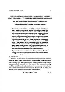
Table 1: Finite sample rejection frequency for DGPs 1-2 (size study, nomial level 0.05) DGP 1
n
T
25
25 50 100 25 50 100
(i) uit P 0.040 0.060 0.056 0.060 0.070 0.034
25 50 100 25 50 100
0.038 0.056 0.058 0.054 0.064 0.038
50
2
25
50
∼ IID N (0, 1) CGL SZ 0.044 0.054 0.044 0.048 0.058 0.064 0.044 0.062 0.052 0.080 0.030 0.048 0.044 0.062 0.044 0.042 0.060 0.052
0.052 0.060 0.064 0.058 0.060 0.052
(ii) uit = 0.5ui,t−1 + εit P CGL SZ 0.092 0.060 0.082 0.130 0.062 0.082 0.126 0.080 0.066 0.118 0.066 0.128 0.112 0.076 0.074 0.124 0.066 0.064 0.088 0.122 0.128 0.076 0.110 0.108
0.050 0.062 0.068 0.078 0.050 0.068
0.090 0.082 0.070 0.120 0.084 0.060
Note: P, CGL, and SZ refer to Pesaran’s, CGL’s and our tests, respectively.
posed in this paper. To conduct our test, we need to choose kernels and bandwidths. To estimate the heterogeneous regression functions, we conduct a third-order local polynomial regression (p = 3) by choosing the second order Gaussian kernel and rule-of-thumb bandwidth: b = sX T −1/9 where sX denotes the sample standard deviation of {Xit } across i and t. To es-
timate the marginal and pairwise joint densities, we choose the second order Gaussian kernel
and rule-of-thumb bandwidth h = suhT −1/6 , where suh denotes the sample standard deviation of {e uit } across i and t. For the CGL test, we follow their paper and consider a local linear re-
gression to estimate the conditional mean function by using the Gaussian kernel and choosing the bandwidth through the leave-one-out cross-validation method. For the Pesaran’s test, we estimate the heterogeneous regression functions by using the linear model, and conduct his CD test based on the parametric residuals. For all tests, we consider n = 25, 50, and T = 25, 50, 100. For each combination of n and
T, we use 500 replications for the level and power study, and 200 bootstrap resamples in each replication. Table 1 reports the finite sample level for Pesaran’s CD test, the CGL test and our test (denoted as P, CGL, and SZ, respectively in the table). When the error terms uit are IID across t, all three tests perform reasonably well for all combinations of n and T and both DGPs under investigation in that the empirical levels are close to the nominal level. When {uit } follows an AR(1) process along the time dimension, we find out the CGL test outperforms
the Pesaran’s test in terms of level performance: the latter test tends to have a large size 17
distortion which does not improve when either n or T increases. In contrast, our test can be oversized when n/T is not small (e.g., n = 50 and T = 25) so that the parameter estimation error plays a non-negligible role in the finite samples, but the level of our test improves quickly as T increases for fixed n. Table 2 reports the finite sample power performance of all three tests for DGPs 3-6. For DGPs 3-4, we have a single-factor error structure. Noting that the factor loadings λi have zero mean in our setup, neither Pesaran’s nor CGL’s test has power in detecting cross-sectional dependence in this case. This is confirmed by our simulations. In contrast, our tests have power in detecting deviations from cross-sectional dependence. As either n or T increases, the power of our test increases. DGPs 5-6 exhibit a two-factor error structure where one of the two sequences of factor loadings have nonzero mean, and all three tests have power in detecting cross-sectional dependence. As either n or T increases, the powers of all three tests increase quickly and our test tends to more powerful than the Pesaran’s and CGL’s tests.
6
Concluding remarks
In this paper, we propose a nonparametric test for cross-sectional dependence in large dimensional panel. Our tests can be applied to both raw data and residuals from heterogenous nonparametric (or parametric) regressions. The requirement on the relative magnitude of n and T is quite weak in the former case, and very strong in the latter case in order to control the asymptotic effect of the parameter estimation error on the test statistic. In both cases, we establish the asymptotic normality of our test statistic under the null hypothesis of cross-sectional independence. The global consistency of our test is also established. Monte Carlo simulations indicate our test performs reasonably well in finite samples and has power in detecting cross-sectional dependence when the Pesaran’s and CGL’s tests fail. We have not pursued the asymptotic local power analysis for our nonparametric test in this paper. It is well known that the study of asymptotic local power is rather difficult in nonparametric testing for serial dependence, see Tjøstheim (1996) and Hong and White (2005). Similar remark holds true for nonparametric testing for cross-sectional dependence. To analyze the local power of their test, Hong and White (2005) consider a class of locally j-dependent processes for which there exists serial dependence at lag j only, but j may grow to infinity as the sample size passes to infinity. It is not clear whether one can extend their analysis to our framework since there is no natural ordering along the individual dimensions in panel data models. In addition, it may not be advisable to consider a class of panel data models for which there exists cross-sectional dependence at pairwise level only: if any two of uit , ujt , and ukt (i 6= j 6= k) are dependent, they tend to be dependent on the other one also.
Thus we conjecture that it is very challenging to conduct the asymptotic local power analysis for our nonparametric test. 18
Table 2: Finite sample rejection frequency for DGPs 3-6 (power study, nomial level 0.05) DGP
n
T
3
25
25 50 100 25 50 100
(i) εit P 0.040 0.060 0.056 0.060 0.070 0.034
25 50 100 25 50 100
0.038 0.056 0.058 0.054 0.064 0.038
0.074 0.052 0.062 0.046 0.068 0.062
0.446 0.772 0.954 0.772 0.970 0.998
0.098 0.206 0.234 0.148 0.190 0.270
0.044 0.066 0.044 0.086 0.072 0.068
0.616 0.858 0.984 0.870 0.990 1.000
25 50 100 25 50 100
0.326 0.412 0.584 0.550 0.720 0.842
0.248 0.332 0.446 0.442 0.620 0.742
0.208 0.444 0.740 0.456 0.812 0.988
0.410 0.486 0.594 0.626 0.754 0.888
0.304 0.350 0.424 0.508 0.640 0.776
0.418 0.672 0.910 0.680 0.918 0.996
25 50 100 25 50 100
0.304 0.428 0.568 0.548 0.724 0.838
0.232 0.330 0.426 0.454 0.636 0.746
0.250 0.424 0.762 0.424 0.814 0.980
0.420 0.488 0.588 0.624 0.760 0.888
0.292 0.348 0.402 0.516 0.636 0.794
0.406 0.634 0.908 0.662 0.908 1.000
50
4
25
50
5
25
50
6
25
50
∼ IID N (0, 1) CGL SZ 0.046 0.446 0.058 0.778 0.074 0.950 0.040 0.772 0.060 0.972 0.064 0.998
(ii) εit P 0.092 0.130 0.126 0.118 0.112 0.124
= 0.5εit−1 + η it CGL SZ 0.052 0.590 0.060 0.860 0.038 0.984 0.070 0.866 0.074 0.992 0.068 1.000
Note: P, CGL, and SZ refer to Pesaran’s, CGL’s and our tests, respectively.
19
APPENDIX Throughout this appendix, we use C to signify a generic constant whose exact value may vary from case to case. Recall PTl ≡ T !/(T − l)! and CTl ≡ T !/ [(T − l)!l!] for integers l ≤ T .
A
Proof of Theorem 3.1 i
i
i
i
i
Recall ϕi,ts ≡ k h,ts −Et [kh,ts ]−Es [k h,ts ]+Et Es [k h,ts ] where k h,ts ≡ k h (uit − uis ) and Es denotes expecR i tation taken only with respect to variables indexed by time s, that is, Es (k h,ts ) ≡ kh (uit − u) fi (u) du. −1 Pn Let ci,ts ≡ E(ϕi,ts ), and cts ≡ (n − 1) i=1 ci,ts . We will frequently use the fact that for t 6= s, δ
δ
ci,ts ≤ Ch− 1+δ αi1+δ (|t − s|)
(A.1) i
as by the law of iterated expectations, the triangle inequality, and Lemma E.2, we have |ci,ts | = |E[k h,ts ] i
i
i
i
i
δ
δ
−Et Es [k h,ts ]| = |E{E[k h,ts |uit ] − Es [k h,ts ]}| ≤ E|E[k h,ts |uit ] − Es [k h,ts ]| ≤ Ch− 1+δ αi1+δ (|t − s|) . Let α (j) ≡ max1≤i≤n αi (j) . Let m ≡ bL log T c (the integer part of L log T ) where L is a large positive
constant so that the conditions on m in Assumption A.1(i*) are all met by Assumption A.1(i). In P δ 1+δ (τ ) = O (1) under Assumption A.1(i). addition, it is obvious that ∞ τ =1 α i j j j Let Zij,t ≡ (uit , ujt ) and ς ij,tsrq ≡ ς (Zij,t , Zij,s , Zij,r , Zij,q ) = k h,ts (kh,ts + k h,rq − 2kh,tr ). Let P P 1 ς ij,tsrq ≡ ς (Zij,t , Zij,s , Zij,r , Zij,q ) ≡ 4! 4! ς ij,tsrq , where 4! denotes summation over all 4! different permutations of (t, s, r, q). That is, ς ij,tsrq is a symmetric version of ς ij,tsrq by symmetrizing over the four time indices and it is easy to verify that ¯ς ij,tsrq
1 i j j j j j j {k h,ts (2k h,ts + 2k h,rq − k h,tr − kh,sr − kh,tq − k h,sq ) 12
=
i
j
j
j
j
j
j
i
j
j
j
j
j
j
i
j
j
j
j
j
j
i
j
j
j
j
j
j
i
j
j
j
j
j
j
+kh,tr (2k h,tr + 2k h,qs − k h,ts − k h,sr − k h,tq − k h,rq ) +kh,tq (2kh,tq + 2k h,sr − k h,tr − k h,qr − kh,ts − kh,sq ) +kh,sr (2k h,sr + 2k h,qt − kh,st − kh,rt − k h,sq − kh,rq ) +kh,sq (2k h,sq + 2k h,rt − k h,st − k h,qt − kh,sr − kh,qr ) +kh,rq (2kh,rq + 2k h,st − k h,rt − k h,qt − kh,rs − kh,qs )}. b nT as Then we can write Γ b nT Γ
= =
1 n (n − 1) 1 n (n − 1)
X
1≤i6=j≤n
X
1≤i6=j≤n
1 PT4 1 CT4
X
(A.2)
ς ij,tsrq
1≤t6=s6=r6=q≤T
X
ς ij,t1 t2 t3 t4 .
(A.3)
1≤t1