Testing EBUASI Class of Life Distribution Based on Goodness of Fit Approach E.A.Radya, E.F.Lashinb and F.A.Abassb a b
Institute of Statistical Studies and Research, Cairo University, Egypt Mathematics Dep., Faculty of Engineering, Tanta University, Egypt
Abstract: Test statistics for testing exponentiality against Exponential Better (Worse) than Used in Average on Specific Interval EBUASI (EWUASI) is proposed based on the goodness of fit approach. The critical values of this test are calculated and tabulated for sample size n=5(1)40, 45, 50. The Pitman asymptotic efficiency (PAE) is discussed and the power of the test for some commonly used distributions in reliability is calculated. Finally real example is presented to illustrate the theoretical results. Key Words: EBUASI, EWUASI, exponential distribution, goodness of fit, Pitman's asymptotic efficiency.
1. INTRODUCTION Concepts of aging describe how a population of units or systems improves or deteriorates with age. Many classes of life distributions are categorized and defined in literature according to their aging is important in any reliability analysis. Testing exponentiality against the classes of life distributions have received a good deal of attention. For testing against new better than used (NBU), we refer to Hollander and Proschan (1972), Koul (1977), Kumazawa (1983) and Ahmad (1994) among others. For testing against decreasing mean residual life (DMRL) we refer to Hollander and Proschan (1975), Langenberg and Srinivasan (1979) and Ahmad (1992) among others. For new better than used in expectation (NBUE), we refer to Koul (1978) and Ahmad et al. (1999) among others. For harmonic new better than used in expectation (HNBUE), we refer to Klefsjo (1982), Abouammoh and Khaliqe (1987), Ahmad (1995) and Hendi et al. (1998) among others. Let X be a nonnegative random variable with distribution function (df) F and a survival function (sf) F = 1 − F . Assume also that X is absolutely continuous with probability density function f and has finite mean µ and variance σ2, both assumed finite. Associated with X is the notion of "random remaining life" at age t, denoted by Xt where Xt has F (x + t) , x, t ≥0. Note that Ft ( x) = F ( x) if and only if F is an exponential distrisf, Ft ( x) = F (t ) bution. Comparing X and Xt in various forms and types create classes of aging. Among these classes are the following: (i) IFR (Increasing Failure Rate) (ii) IFRA (Increasing Failure Rate Average) (iii) NBU (New Better than Used) (iv) NBUE (New Better than Used in Expectation) (v) HNBUE (Harmonic New Better than Used in Expectation) For definitions of these classes and further details see, e.g. Barlow and Proschan (1981).
Correspondence
[email protected] 1
Definition 1.1: Let X and Y be two random variables with (marginal) df's F and G, respectively. We say that X is less variable than Y (or X is increasing ordering in concave (icv) than Y), and we write X ≤ icv Y iff
∫
x
0
x
F (u )du ≤ ∫ G (u )du . 0
And we say that X is increasing ordering in convex (icx) than Y, and we write X ≤ icx Y iff
∫
∞
x
∞
F (u )du ≤ ∫ G (u )du , for all x≥0 x
∞
and µ = ∫ F (u )du . 0
The increasing ordering in concave (icv) is related to increasing ordering in convex (icx) as given in the following theorem. Theorem 1.1: Let X and Y be two random variables with distribution F and G, respectively
with F (0- ) = G (0- ) =0 and
∫
∞
∞
F (u )du = ∫ G (u )du (i.e. F and G have the same mean), then,
0
0
X ≤ icv Y ⇔ X ≤ icx Y or F ≤ icv G ⇔ F ≤ icx G For proof of this theorem see Hendi et al. (1999). Definition 1.2: The non-negative random variable X with distribution F is said to be exponential better than used ordering (EBU) if X t ≤ icv X for all t≥0. In such a case we write X ∈ EBU (or F ∈ EBU ), iff
Ft (u ) ≤ e −u / µ or F (u + t ) ≤ F (t )e − u / µ See Elbatal (2002). Definition 1.3: The non-negative random variable X with distribution F is said to be exponential better than used in average ordering (EBUA) if X t ≤ icv X for all t≥0. In such a case we write X ∈ EBUA (or F ∈ EBUA ). Its dual class is exponential worse than used in average ordering (EWUA) which is defined by X t ≥ icv X for all t≥0. The above inequalities are equivalent to
∫
x
0
x
Ft (u ) ≤ (≥) ∫ e −u / µ du ; t≥0, x>0 0
or x
x
0
0
−u / µ ∫ F (u + t )du ≤ (≥) F (t )∫ e du ; t≥0, x>0
See Attia et al. (2005).
2
∞
Definition 1.4: A distribution function F with support [0, ∞) and finite mean µ = ∫ F (u ) du , is 0
called Exponential Better (Worse) than Used in Average at Specific Interval EBUASI (EWUASI) if y+x
∫ F (t + u ) du
y+ x
≤ ( ≥ ) F (t )
y
∫e
−u / µ
du
y
This class of life distribution is presented by Abdul-Moniem (2007), for the relationship between this class and other classes like EBU, EBUC, EBUA and NBUE see Abdul-Moniem (2007). This paper is organized as follows, in section 2, we present a test statistic based on goodness of fit approach for testing Ho: F is exponential against H1: F is EBUASI and not exponential and large sample properties also presented, in section3 Pitman's asymptotic efficiency (PAE) of the test for some common distribution are tabulated, in section 4 Monte Carlo Critical points are obtained for sample sizes n= 5(1)40, 45, 50, and power of the test is estimated in section 5. Finally applications using real data are also introduced in section 6.
2-Testing Exponentiality against EBUASI class In this section a test statistic based on the goodness of fit approach is developed to test Ho: F is exponential against H1: F is EBUASI and not exponential. Lemma 2.1 If F is EBUASI then a measure of departure from Ho is ∆ where,
⎡ 1 3 3 ⎤ ∆ = E⎢ X 2 e − X / µ + Xe − X / µ + µ e − X / µ − µ ⎥ 4 4 ⎦ ⎣ 2µ
(2.1)
Proof:
The EBUASI (EWUASI) class of life distribution is defined as, y+x
∫ F (t + u ) du
y+ x
≤ ( ≥ ) F (t )
y
∫e y
Then ∞
∞
y +t
y + x +t
∫ F (u)du −
∫ F (u)du ≤ (≥)µ F (t )(e
−y / µ
− e (− y − x ) / µ )
Define ∞
v( y + t ) =
∫ F (u)du
∞
and
v( y + x + t ) =
y +t
∫ F (u)du
y + x +t
Then v ( y + t ) − v ( y + x + t ) ≤ ( ≥ ) µ F (t ) e − y / µ − e (− y − x ) / µ
(
3
)
−u / µ
du
Define a measure of departure from Ho as ∞∞∞
[
(
]
)
∆ = ∫ ∫ ∫ µ F (t ) e − y / µ − e (− y − x ) / µ − v( y + t ) + v( y + x + t ) dFo ( x)dFo ( y )dFo (t ) 0 0 0
1 1 Where dF o ( x ) = 1 e − x / µ dx , dFo ( y ) = e − y / µ dx , dFo (t ) = e −t / µ dx
µ
µ
µ
Let ∆ =I1-I2+I3 I1 =
∞∞∞
∫ ∫ ∫ µ F (t )(e
1
µ
3
−y / µ
)
− e (− y − x ) / µ e − x / µ e − y / µ e −t / µ dxdydt
0 0 0
∞
I1 = I1 =
I2 = I2 = I2 =
X
1 1 I ( X > t ) e − t / µ dt = E ∫ e − t / µ dt 4 ∫0 4 0
µ
[
E 1 − e−X / µ
4
1
µ
3
]
∞∞∞
∫ ∫ ∫ v ( y + t )e
−x / µ
e − y / µ e −t / µ dxdydt
0 0 0
1
µ2 1
µ2
∞∞
∫ ∫ ( X − y − t )I ( X > y + t )e X X −y
E∫ 0
∫ ( X − y − t )e
−y / µ
e −t / µ dtdy
0
[
I3 = I3 =
1
µ3 1
µ3 1
µ3
e −t / µ dtdy
0 0
I 2 = E 2 µe − X / µ + X + Xe − X / µ − 2 µ
I3 =
−y / µ
∞∞∞
∫ ∫ ∫ v ( y + x + t )e
−x / µ
]
e − y / µ e −t / µ dxdydt
0 0 0
∞∞∞
∫∫∫
( X − y − x − t )I ( X > y + x + t )e − y / µ e − x / µ e −t / µ dtdxdy
0 0 0
X X − y X − y−x
E∫ 0
∫ ∫ 0
( X − y − x − t )e − y / µ e − x / µ e −t / µ dtdxdy
0
⎡ ⎤ 1 2 −X / µ − 3µ ⎥ I 3 = E ⎢3µe − X / µ + X + 2 Xe − X / µ + X e 2µ ⎣ ⎦ From I1, I2, and I3 ⎡ 1 3 3 ⎤ X 2 e − X / µ + Xe − X / µ + µ e − X / µ − µ ⎥ ∆ = E⎢ 4 4 ⎦ ⎣ 2µ Then the proof is completed.■ Based on a random sample X1,……,Xn with mean x from a distribution F, a direct empirical estimate of the measure ∆ in (2.1) is:
1 ∆ˆ = n
n
⎡1
∑ ⎢⎣ 2 x i =1
2 i
e − xi + x i e − xi +
3 − xi 3 ⎤ − ⎥ e 4 4⎦
4
(2.2)
The following theorem gives the large sample properties of the test statistic ∆. Theorem 2.1 As n→ ∞,
n (∆ˆ − ∆ ) is asymptotically normal with mean 0 and variance σ2, where
σ2 under Ho is given by σ2o=0.02 Proof:
It is straightforward, by noting that ∆ˆ is just an average of ∆, then using the central limit theorem the result follows. The variance will be ⎡ 1 3 3 ⎤ σ 2 = Var ⎢ X 2 e − X / µ + Xe − X / µ + µe − X / µ − µ ⎥ 4 4 ⎦ ⎣ 2µ under Ho the variance becomes, ⎡
1
7
3
9
3
3
9
9⎤
σ o2 = E ⎢e −2 x ( x 3 + x 4 + x 2 + x + ) − e − x ( x 2 + x + ) + ⎥ = 0.02 ■ 4 4 2 16 4 2 8 16 ⎦ ⎣ To perform the above test, reject Ho if the value of (n 0.02 )∆ˆ will exceeds Zα which is the upper percentile of the standard normal variety.
3- Pitman Asymptotic Efficiency (PAE) The pitman asymptotic efficiency of the class EBUASI was calculated using the Linear Failure Rate (LFR), Makeham, and Weibull distributions. The pitman efficiency is defined as: PAE =
µ ′(θ o ) ⎛⎜ ∂∆ = ⎜ ∂θ σo ⎝
θ =θ o
⎞ ⎟ σ o ⎟ ⎠
The following three families of alternatives are often used for efficiency calculation •
Linear Failure Rate : F θ ( x ) = e
•
Makeham :
Fθ ( x ) = e − x − θ ( x + e
−x
− x −
1 θx 2
2
−1)
− xθ
• Weibull : F θ ( x ) = e The null exponential is attained at θ= 0, 0 and 1 respectively. The efficiency calculation for the above three alternatives are tabulated in table I. Table-I Pitman Asymptotic efficiency Distribution
Efficiency
LFR
0.220
Makeham
0.114
Weibull
0.910
4- Monte Carlo Null Distribution Critical Points
In this section a simulation for the null distribution critical points for ∆ˆ will be made for sample sizes n=5(1)40, 45, 50 from the standard exponential distribution. Table-II gives the upper percentile of the statistic ∆ˆ ; the followed figure shows the relation between the critical values and the sample size. 5
Table II: Critical values of ∆ˆ n 5 6 7 8 9 10 11 12 13 14 15 16 17 18 19 20 21 22 23 24 25 26 27 28 29 30 31 32 33 34 35 36 37 38 39 40 45 50
90% 0.064 0.062 0.059 0.055 0.054 0.052 0.052 0.049 0.046 0.046 0.045 0.043 0.042 0.039 0.039 0.038 0.038 0.037 0.035 0.036 0.035 0.034 0.034 0.033 0.031 0.031 0.031 0.031 0.031 0.030 0.028 0.028 0.029 0.028 0.027 0.027 0.025 0.024
95% 0.070 0.069 0.066 0.062 0.061 0.060 0.059 0.055 0.055 0.054 0.053 0.052 0.049 0.048 0.047 0.046 0.045 0.044 0.043 0.042 0.042 0.041 0.041 0.040 0.039 0.037 0.038 0.037 0.038 0.036 0.034 0.035 0.035 0.035 0.034 0.034 0.031 0.031
98% 0.076 0.074 0.072 0.069 0.068 0.065 0.066 0.062 0.062 0.060 0.060 0.059 0.059 0.054 0.055 0.052 0.051 0.051 0.051 0.051 0.050 0.049 0.049 0.048 0.046 0.046 0.044 0.045 0.044 0.042 0.041 0.040 0.043 0.041 0.039 0.040 0.038 0.036
99% 0.081 0.079 0.075 0.072 0.071 0.069 0.068 0.066 0.066 0.064 0.064 0.062 0.063 0.059 0.059 0.056 0.057 0.054 0.055 0.055 0.054 0.052 0.052 0.052 0.049 0.051 0.049 0.049 0.048 0.045 0.046 0.044 0.047 0.044 0.044 0.043 0.042 0.041
Relation between critical values and sample size for ∆ˆ
Critical Values
0.08
90% 95% 98% 99%
critical critical critical critical
values values values values
0.06
0.04
0.02 0
20
40
Sample Size
6
60
5- Power of the test In this section an estimation of the power for testing exponentiality versus EBUASI will be made using significance level 95% with suitable parameters values of θ at n=10,20,and 30, and for commonly used distributions in reliability such as LFR, Makeham, and Weibull alternatives. Table-III shows the power of the test. Table-III: Power estimates Distribution LFR Makeham Weibull
θ 2 3 4 2 3 4 2 3 4
10 0.567 0.632 0.627 0.393 0.514 0.559 0.475 0.879 0.988
n 20 0.963 0.990 0.993 0.811 0.939 0.977 0.854 1 1
30 1.00 1 1 0.970 0.998 1 0.982 1 1
6-Applications The following data represent 39 liver cancer's patients taken from El Minia Cancer Center of Ministry of Health of Egypt, in 1999. The ordered life times (in days) are: (i) The data are: 10, 14, 14, 14, 14, 14, 15, 17, 18, 20, 20, 20, 20, 20, 23, 23, 24, 26, 30, 30, 31, 40, 49, 51, 52, 60, 61, 67, 71, 74, 75, 87, 96, 105, 107, 107, 107, 116, and 150. It is found that the test statistic for the set of data by using equation (2.2) is ∆ˆ = -0.75 which is less than the critical value of the table I, then we accept Ho which states that the set of data don not have EBUASI property at 95% percentile.
Acknowledgment The authors would like to thank prof. M. I. Hendi for his helpful comments, which improved the presentation of the paper.
References Abdul-Moniem, I. (2007). A new class of aging distributions. J. Egypt. Statist. Soc., 23, 124. Abouammoh, A.M. and Khalique, A. (1987). Some tests for mean residual life criteria based on total time on test transform. Reliability Engineering, 19, 85-101. Ahmad, I. A., Hendi, M. I., Al-Nachawati, H. (1999). Testing new better than used class of life distribution derived from convex ordering using kernel method. J. Nonparametric Statist., 11, 393-411. Ahmad, I. A. (1995). Nonparametric testing of class of life distributions derived from a variability ordering. Parisankhyan Samikka, 2, 13-18.
7
Ahmad, I. A. (1994). A class of statistics useful in testing increasing failure rate average and new better than used life distributions. J. Statist. Plant. Inf., 41, 141-149. Ahmad, I. A. (1992). A new test for mean residual life time. Biometrika, 79, 416-419. Attia, A. F., Mahmoud, M. A. W. and Abdul-Moniem, I. (2005). "The class of exponential better than used in average". The 40th Annual Conference on statistics, Computer science and Operations Research, Cairo Uin. Barlow, R. E. and Proschan, F. (1981). "Statistical theory of reliability and life testing". To Begin With, Silver-Spring, MD. Elbatal, I. I. (2002). "The EBU and EWU classes of life distribution". J. Egypt. Statist. Soc., 18, 59-80. Hendi, M. I., Al-Nachwati, H. Montasser, M. and Alwasel, I. A. (1998). An exact test for HNBUE class of life distribution. J. Statist. Compu. Simul., 60, 261-275. Hendi, M. I., Al-Nachwati, H. and Al-Ruzaiza, A. S. (1999). A test for exponentiality against New Better than Used Average. J. King Saud Uni. 11, 107-121. Hollander, M. and Proschan, F. (1972). Testing whether new better than used. Ann. Math. Statist.., 43, 1136-1146. Hollander, M. and Proschan, F. (1975). Test for mean residual life. Biometrika, 62, 585-593. Koul, H. I. (1977). A new test for new better than used. Comm. Statist. Theor. Meth., 6, 563573. Koul, H. I. (1978). Testing for new better than used in expectation. Comm. Statist. Theor. Meth., 7, 685-701. Kumazawa, Y (1983). Testing for new is better than used. Comm. Statist. Theor. Meth., 12, 311-321. Klefsjo, B. (1982). The HNBUE and HNWUE class of life distributions. Naval Res. Logistics Quarterly, 21, 331-344. Langenberg, P. and Srinivasan, R. (1979). Null distribution of the Hollander and Proschan statistic for decreasing mean residual life. Biometrika, 66, 679-680.
8