Oct 10, 2012 - the structure formation in both the spatially flat and curved Universe. We also .... The first term in Eq.(10) is divergent when x goes to the minus ...
Testing f (R) dark energy model with the large scale structure Jian-hua He1
arXiv:1207.4898v2 [astro-ph.CO] 10 Oct 2012
1
INAF-Osservatorio Astronomico di Brera, Via Emilio Bianchi, 46, I-23807, Merate (LC), Italy
In this work, we further investigate the family of f (R) dark energy models that can exactly mimic the same background expansion history as that of the ΛCDM model. We study the large scale structure in the f (R) gravity using the full set cosmological perturbation equations. We investigate the structure formation in both the spatially flat and curved Universe. We also confront our model with the latest observations and conduct a Markov Chain Monte Carlo analysis on the parameter space. PACS numbers: 98.80.-k,04.50.Kd
I.
INTRODUCTION
There has been accumulated conclusive evidence from supernovae[1] and other observations[2, 3] in the last decade, indicating that our Universe is undergoing a phase of accelerated expansion. Understanding the nature of the cosmic acceleration is one of the biggest questions in modern physics. The leading explanation of the accelerated expansion is the cosmological constant within the context of General Relativity. However, the measured value of cosmological constant is far below the prediction of any sensible quantum field theories and the cosmological constant will inevitably lead to the coincidence problem that why the energy density of matter and vacuum are in the same order today(see [4] for review). Another possibility for the acceleration is that the universe is driven by a new and yet-unknown component called dark energy. The dark energy is some kind of dynamical fluid with negative and time-dependent equation of state w(a). However, the nature of the dynamical dark energy is even harder to be understood in the fundamental physics than that of the cosmological constant. Alternatively, a promising explanation of the acceleration is the modified gravity. The General relativity might not be ultimately correct in the cosmological scale. The Universe might be described by some kind of modified gravity. One simplest attempt is called f (R) gravity, in which the scalar curvature in the Lagrange density of Einstein’s gravity is replaced by an arbitrary function of R[5]. The f (R) gravity can produce the accelerated expansion of the Universe with any designed effective dark energy equation of state w[6]. Furthermore, the time dependent effective DE EoS in the Jordan frame can be reproduced from the dilation of the inertial mass in the Einstein frame through the conformal transformation [7][8][9]. In this sense, the time dependent dark energy phenomenon can be better understood in a physical way in the framework of modified gravity. In this paper, we investigate a specific family of f (R) models that can reproduce the same background expansion history as that of the ΛCDM model since it has been argued that a valid f (R) model should closely math the ΛCDM background[10]. The family of f (R) model con-
tains only one more extra parameter than that of the ΛCDM model and furthermore, it does have the welldefined Lagrangian formalism in the spatially flat Universe, which is valid for the whole expansion history of the Universe from the past to the future. The model is no longer simply a phenomenological model. Although this model has been studied by a number of work within the parameterized framework of modified gravity [11] [12], it still needs to solve the full set of cosmological perturbation equations to get more accurate results on the scale k dependent growth history of the Universe when confronted with upcoming high precision data in cosmological surveys. Therefore, in this work, instead of using the parameterized framework of modified gravity, we investigate the impact of f (R) models on the large scale structure using the full set of covariant cosmological perturbation equations. We will confront our f (R) model with the latest observations and conduct a Markov Chain Monte Carlo analysis on the parameter space. We will also exploit the spatially non-flat case in the f (R) gravity, which has not been addressed in the previous work [12] [13] [14]. This paper is organized as follows: In section II, we review the background dynamics of the Universe in the f (R) gravity and present the well-defined Lagrangian formalism in the spatially flat Universe for the family of f (R) models that reproduce the ΛCDM background expansion history. In section III, we present the scalar perturbation equations in the synchronous gauge for the f (R) gravity and study the impact of f (R) gravity on the large scale structure formation. In section IV, we present the fittings results by confronting our model with the latest observations. In section V, we summarize and conclude this work. II.
THE BACKGROUND DYNAMICS
We work with the 4-dimensional action in the f (R) gravity[15] Z Z √ 1 S = 2 d4 x −gf (R) + d4 xL(m) , (1) 2κ where κ2 = 8πG. We consider a homogeneous and isotropic background universe described by the
2 Friedmann-Robertson- Walker(FRW) metric ds2 = a2 [−dτ 2 + dσ 2 ] ,
(2)
where dσ 2 is the conformal space-like hypersurface with a constant curvature R(3) = 6K dσ 2 =
dr2 + r2 (dθ2 + sin2 θdφ2 ) . 1 − Kr2
(3)
The dynamics of the Universe in the f (R) gravity is described by[15] 2K F¨ + 2F H˙ − H F˙ − 2 F = −κ2 (ρ + p) . a
(4)
(R) where F = dfdR , the dot denotes the time derivative with respect to the cosmic time t and ρ is the total energy density of the matter which consists of the cold dark matter, baryon and radiation ρ = ρc + ρb + ρr . p is the total pressure in the Universe. If we convert the derivatives in Eq.(4) from the cosmic time t to x = ln a , Eq.(4) can be recast into
1 d ln E dF d ln E 2K −2x d2 F +( − 1) +( − e )F 2 dx 2 dx dx dx E (5) κ2 dρ = , 3E dx where H2 , H02 dE R ≡ 3( + 4E) + 6Ke−2x dx dρ = −3(ρ + p) . dx E≡
(6)
,
For convenience, the energy density ρ, K and the scalar curvature R in Eq.(5) are in the unit of H02 and we also set κ2 = 1 in our analysis. In order to get a viable f (R) model with a reasonable expansion history of the Universe and without loss of generality, we can parameterize the quantity E(x) in Eq.(5) as the standard model in Einstein’s gravity with an effective dark energy equation of state(EoS) w[6][16] E(x) = Ω0r e−4x + Ω0m e−3x + Ω0k e−2x + Ω0d e−3
Rx 0
(1+w)dx
E(x) = Ω0m e−3x + Ω0d
.
Ω0k ≡ −
(8)
(9)
In this case, Eq.(5) can be solved analytically. The general solutions for Eq.(5) are Ω0d ] Ω0m (10) 0 3x p+ 3x Ωd ] , + D(e ) 2 F1 [q+ , p+ ; r+ ; −e Ω0m
F (x) − 1 = C(e3x )p− 2 F1 [q− , p− ; r− ; −e3x
where the indexes in the above expressions are given by √ 1 ± 73 q± = , 12 √ 73 r± = 1 ± , √6 5 ± 73 . p± = 12 2 F1 [a, b; c; z] is the Gaussian hypergeometric function. C and D are arbitrary constants. A viable f (R) model should be in a “chameleon” type [17][18] where in the past of the Universe, the model should go back to the standard model
lim F (x) = 1 .
, (7)
where K , H02 κ2 ρ0m , Ω0m ≡ 3H02 κ2 ρ0d Ω0d ≡ , 3H02 κ2 ρ0r Ω0r ≡ . 3H02
ρ0d indicates the energy density of the effective dark energy, ρ0m = ρ0b +ρ0c is the energy density of non-relativistic matter and ρ0 = ρ0m + ρ0r is the total energy density of the matter. The f (R) model can be constructed by specifying the background expansion history of the Universe in Eq.(5). Eq.(5) becomes a second order differential equation only with respect to F (x). However, any specifically designed time dependent effective dark energy equation of state can hardly be well motivated in physics because we still have less knowledge about the nature of the dark energy at present. Therefore, it is of great interest to investigate the simplest case that the f (R) model can reproduce the same background expansion history as that of the ΛCDM model w = −1. Therefore, in this work we will only focus on this case hereafter. In the spatially flat Universe K = 0 filled with dust matter, the late time expansion history of the Universe with the effective dark energy EoS w = −1 can be written as,
(11)
x→−∞
The first term in Eq.(10) is divergent when x goes to the minus infinity due to the negative index p− and C, therefore, should vanish C = 0 to satisfy the boundary condition Eq.(11). After we get the expression for F (x), we can obtain the explicit expression for f (R) by doing the integration Z dR dx , (12) f (R) = F (x) dx and using the relationship between R and x. R = 3Ω0m e−3x + 12Ω0d
.
(13)
3 The final result for f (R) turns out to be 0.0
f (R) = R − 2Λ � �p+ −1 � � , Λ Λ −̟ 2 F1 q+ , p+ − 1; r+ ; − R − 4Λ R − 4Λ (14) where Λ, ̟ are constant parameters. p+
̟ = D(R0 − 4Λ)
/(p+ − 1)/Λ
f (R) ∼ R − ̟
Λ R
�p+ −1
f HRL - R -0.4 R
p+ −1
.
(15)
When ̟ = 0, Λ is just the cosmological constant. If we write Eq.(14) in the units of H02 , R0 and Λ can be presented as R0 = (3Ω0m + 12Ω0d) and Λ = 3Ω0d respectively. The hypergeometric function 2 F1 [a, b; c; z] can have the integral representation on the real axis when b > 0 and c>0 Z 1 Γ(c) F [a, b; c; z] = tb−1 (1−t)c−b−1 (1−zt)−a dt 2 1 Γ(b)Γ(c − b) 0 (16) where Γ is the Euler Gamma function. In this case, 2 F1 [a, b; c; z] is well-defined in the range −∞ < z < 1 The expression of Eq.(14), therefore, is a well-defined real function on the real axes in the physical range R > 4Λ, which is different from the results given by [19]. A more detailed analysis on Eq.(14) has been presented in our companion work [20]. In the past of the Universe, when R >> 4Λ, the hypergeometric function goes back to unity 2 F1 ∼ 1, and Eq.(14) becomes �
-0.2
.
(17)
The above expression can further go back to the standard model f (R) ∼ R when R becomes more larger. On the other hand, in the future expansion, Eq.(14) does not have the future singularity because f (R) is finite at the point of R = 4Λ. lim f (R) = 2Λ−
R→4Λ
√ ̟4(−511 + 79 73)Γ(2/3)Γ(−r− ) √ √ √ (−5 + 73)(−1 + 73)(7 + 73)Γ(−p− )Γ(q+ ) ≈ 2Λ − 1.256̟
.
(18)
When R < 4Λ the expression of Eq.(14) becomes complex, which is clearly unphysical. In the spatially flat Universe, Eq.(14) is valid for the whole expansion history of the Universe from the radiation dominated epoch to the future expansion of the Universe. Eq.(14) can exactly mimic the ΛCDM expansion history from the matter dominated epoch to the late time acceleration. For illustrative propose, in Fig. 1, we plot the f (R) models for a few representative values of D. The curves in Fig. 1 are evaluated from Eq.(14) directly. By noting the different conventions of f (R) used
-0.6
-0.8 10
20
50
100
200
500
1000
R H02
, FIG. 1: The f(R) models that can reproduce the ΛCDM expansion history. From top D = −0.6, −0.4, −0.2, 0, 0.2, 0.4, 0.6 and Ω0m = 0.24 in our work and [6], our results are consistent with the numerical results presented in [6]. As shown in [21], in order to avoid the instabilities in the high curvature region, it requires that F > 0 and ∂F fRR = ∂R > 0. Therefore, in our model D should be negative D < 0. The models presented in the red dashed lines in Fig. 1(D > 0) are ruled out by the instabilities in the high curvature region. Since the f (R) model investigated in our work has only one more extra parameter than that of the ΛCDM model, the family of f (R) models can be characterized by either D or dH dR B0 = fRR F dx H/ dx (x = 0)[6]. In the appendix, we provide the explicit relationship between B0 and D. However, in this work, we are not only limited in the spatially flat Universe, we will also exploit the f (R) model in the spatially curved Universe. Without losing generality, we will numerically find the solution of Eq.(5) to include the spatially curved case Ω0k 6= 0. We perform our numerical calculation starting from the deep matter dominated epoch(ai ∼ 0.03). The curvature term K can be neglected at this epoch and the analytical solutions for Eq.(5) give rise to F (x) ∼ 1 + D(e3x )p+ , (19) dF (x) ∼ 3Dp+ (e3x )p+ , dx We take the above expressions as the initial conditions for Eq.(5). In this work, we use the parameter D to characterize the family of f (R) models and treat B0 as derived parameter since D directly relates to the covariant parameter ̟ for this kind of f (R) models in the spatially flat Universe. Since the f (R) model investigated in our work and the ΛCDM model can only be distinguished in their perturbed space-time, in the next section, we will turn to the cosmological perturbations theory.
4 III.
COSMOLOGICAL PERTURBATIONS
The cosmological perturbation theory for the f (R) gravity has been well studied in [22]. [22] has extensively presented the perturbation equations for a wide family of modified gravities. The perturbation equations in the spatially flat Universe for the f (R) gravity can be found in [23]. For the scalar perturbation, the perturbed line element can be written as[24] (s)
ds2 = a2 [−(1 + 2ψY (s) )dτ 2 + 2BYi dτ dxi (s)
+ (1 + 2φY (s) )γij dxi dxj + EYij dxi dxj ] ,(20) where γij in the spherical coordinate can be written as
[γij ] =
1 1−Kr 2
0 0
,
α≡
=
(22)
(29)
k2 + M 2 )δF a2
κ2 a2 1 (δρ − 3δp) − F ′ h′L 3 2
,
(30)
where
.
M2 =
In this work, we focus on the synchronous gauge which is defined by ψ = 0 and B = 0. The synchronous gauge is widely used in the Einstein-Boltzmann codes [25] [26] [27] [28] to calculate the temperature and polarization power spectra of the cosmic microwave background anisotropy. The synchronous gauge is characterized by the following two parameters ,
hL = 6φ ,
(23)
where ηT refers to the conformal 3-space curvature perturbation δR(3) = 6δK = −4(k 2 − 3K)ηT
,
and δF ′′ + 2HδF ′ + a2 (
The detailed general covariant perturbation equations including the spatially curved case for the f (R) gravity are presented in the appendix.
E ) 6
(hL + 6ηT )′ 2k 2 q = (ρ + p)v
(21)
Y ,Yj and Yij are the scalar harmonic functions which are defined by
ηT = −(φ +
1 1 3 1 1 − κ2 a2 δρ = −( F H + F ′ )h′L − HδF ′ − δF k 2 2 2 4 2 2 3 ′ 2 (25) + F ηT (k − 3K) + H δF , 2 2 2 1 κ2 a2 δp = F [− Hh′L + k 2 ηT − h′′L − 2ηT K] 3 3 3 2 1 a′′ − k 2 + 2K] − F ′ h′L + δF [H2 + a 3 3 − δF ′′ − δF ′ H , (26) ′ δF pΠ F − α − κ2 a2 , α′ = −2Hα + ηT − F F k2 F (27) 2 ′ k − 3K ′ 1 1 1 F hL K F ηT = κ2 a2 q + kδF ′ − kHδF + , k 2 2 2 2k (28) where
0 0 r2 0 0 r2 sin2 θ
(∆ + k 2 )Y (s) = 0 , 1 (s) (s) , Yj ≡ − Y|j k 1 (s) 1 (s) Yij ≡ 2 Y|ij + γij Y (s) k 3
chronous can be written as
.
(24)
The perturbed modified Einstein equations in the syn-
1 F − R) . ( 3 fRR
(31)
The scalar curvature perturbation δR is given by a2 δR = h′′T + 3Hh′T − 4ηT k 2 + 12KηT
.
(32)
With the perturbation equations, we perform our numerical analysis based on the public available EinsteinBoltzmann code CAMB [27]. In the appendix, we summarize the details on how to modify the code. In Fig.2, we show the full spectrum of temperature anisotropy ClT T for a few representative values of D. The cosmological parameters used in the numerical process are taken from the WMAP 7-year best-fitted values for the ΛCDM model [2] Ωb h2 = 0.0227, Ωch2 = 0.112, ns = 0.966, ∆2R = 2.42 × 10⁻⁹ , ΩΛ = 0.729, τ = 0.085 . From Fig.2, we can see that the f (R) gravity only affects the lowest multipoles in the power spectrum while not change the acoustic peaks. This observation is consistent with what found in[6]. The small l power is suppressed as the decreasing of the value of D. However, there is a turning around point, roughly about D < −0.37(B0 > 1.5), after which there is a prominent enhancement in the power as further decreasing the value of D. Numerical results of our work agree with the already presented results within the parameterized framework of modified gravity[11][12].
5
z=0
D=-1.5 (B =33.4)
)]
/(2 )[ K ]
0
3
2
D=-1.2
Mpc
(B =12.3)
4
10
(
D=0
CDM)
0
0
0
10
CDM)
D=-1E-3 (B =3.24E-3)
D=-0.1 (B =0.344)
3
(
D=-1E-4 (B =3.24E-4)
L
D=0
P (k)
l(l+1)C
l
[(h
TT
-1
0
3
10
D=-0.2 (B =0.732)
D=-1E-2 (B =3.24E-2) 0
0
D=-0.3 (B =1.17) 0
101
102
-4
103
10
-3
10
in Fig 4, we show the two-point correlation function in the real space. We can see clearly that although the shape of the correlation function has changed a lot for a few representative values of D, the position of the BAO peak does not change under the Fourier transformation, which shows that our numerical results are consistent with the theoretical prediction. In the spatially curved Universe, Ω0k has significant impact on both the matte power spectrum and the CMB angular power spectrum. In the matter power spectrum, as shown in Fig.5, the positive Ω0k > 0 will suppress the power at all scales and the negative Ω0k < 0 will oppositely enhance the power. The slight positive value of Ω0k > 0 could compensate part of the impact induced by the modified gravity D on the matte power spectrum, which enhance the power at scale k > 0.001hMpc−1 (see Fig.3). Meanwhile, the spatial curvature Ω0k also shifts the positions of acoustic peaks in the CMB temperature angular power spectrum. However, the high precision measurement of the acoustic peaks in the CMB temperature angular power spectrum in combination with BAO
-1
10
0
10
-1
FIG. 2: The angular power spectrum of the temperature correlation
In Fig.3, we show the linear matter power spectrum at redshift zero z = 0. The f (R) gravity changes not only the amplitude but also the shape of the power spectrum due to the scale k dependent growth history [6]. However, the f (R) model investigated in our work should not change the position of the Baryon Acoustic Oscillation(BAO) peak in the two-point correlation function in the real space because the sound horizon is only determined by the background cosmological parameters[29][30] and the family of f (R) models investigated in our work has the same background expansion. By doing the Fourier transformation Z 1 sin(kr) ξ(r) = , (33) dkk 2 PL (k) 2π 2 kr
-2
10
k[h Mpc ]
l
FIG. 3: The linear matter power spectrum.
and H0 [2] can put very tight constrains on the spatial curvature. The spatial curvature, therefore, could not affect significantly on the large scale structure in the f (R) gravity. Compared with the CMB temperature angular power spectrum ClT T (see Fig.2), there are no significant imprint of f (R) gravity on the temperature polarization cross-correlation and polarization auto-correlation spectrum ClT E ,ClEE (see Fig.6) because the CMB polarization anisotropy only arises from the quadrupole anisotropy at the last scattering surface and does not correlate with the late time ISW effect. There are no gravitational perturbation terms appearing in the source term SE for the polarization correlation. For instance, in the spatially flat Universe, SE can be written as [31][32] SE =
gζ − τ )2
4k 2 (τ0
,
(34)
where g is the visibility function and ζ is given by ζ = ( 34 I2 + 92 E2 ). I2 , E2 indicate the quadrupole of the photon intensity and the E-like polarization respectively [32]. After the last scattering, the visibility function g ≃ δ(τ − τdec ) drops almost to be zero. The perturbation of the f (R) gravity has no impact on SE unless the f (R) model changes the background expansion. After the qualitative analysis of the impact of f (R) model on the large scale structure, in the next section, we will present cosmological constrains on the f (R) model from the latest observations.
IV.
CONSTRAINS FROM OBSERVATIONS
The parameter space of our model is P = (Ωb h2 , Ωc h2 , θA , Ωk , ln[1010 As ], ns , τ, D) ,
(35)
200
D=0
2
/2 [ k ]
6
D=0
0.010
(
CDM)
D=-1E-4 (B =3.24E-4)
TE
l
0
l(l+1)C
D=-1E-3 (B =3.24E-3) 0
D=-1E-2 (B =3.24E-2) 0
CDM)
D=-0.1 (B =0.344)
100
D=-0.2 (B =0.732)
0
0
D=-0.3 (B =1.17)
50
0
0 -50 -100 -150
0.005
40
l(l+1)C
EE
l
2
/2 [ k ]
(r)
(
150
0.000
60
80
100
120
140
200
-1
3
P (k)[(h Mpc) ]
D= -0.01
-1
4
L
k
k
k
10
=-0.1 =0 =0.1 =0.2
3
10
-3
10
-2
400
600
800
1000
1200
1400
1600
1800
2000
l
FIG. 4: The two-point correlation function in the real space
k
0
160
r[Mpc h ]
10
20
10
-1
-1
k[h Mpc ]
FIG. 5: The impact of the curvature Ωk on the matter power spectrum
where θA is the angular size of the acoustic horizon, and As is amplitude of the primordial curvature perturbation. The priors for cosmological parameters are listed in table I. For the CMB data, we use the sevenyear WMAP(WMAP 7) CMB temperature and polarization power spectra [2]. We also take the measurement of the power spectrum of LRG from SDSS DR7 [33]. However, we limit our considerations of the matter power spectrum in a relative linear scale and we only take the samples within bins for k < 0.1h/Mpc. We add the supernovae data [34] and the present day value of the Hubble constant from the measurement of Hubble Space Telescope(HST) H0 = 74.2 ± 3.6kms−1 Mpc−1 [35] in order to put tighter constrains on the background cosmological parameters. The global fitting results using
FIG. 6: The TE and EE angular power spectrum.
above data sets are listed in Table II and III. In the flat Universe, we find the constrains on the parameter D as |D| < 0.709(95%CL) and |D| < 0.711(95%CL) in the curved Universe. These results are equivalent to B0 < 3.86(95%CL) and B0 < 3.88(95%CL) if we use the parameter B0 . The result is consistent with [13]. Although the f (R) gravity has significant impact on the shape of the matter power spectrum(see Fig. 3), the SDSS LRG matter spectrum can not put very tight constrains on D because there are degeneracies between D and other cosmological parameters[13]. When D ∼ −0.6(B0 ∼ 3), the CMB temperature angular power spectrum ClT T of the f (R) model goes back similar to that of ΛCDM model. Therefore, there are two peaks in the likelihood distribution of D which are clearly shown in the black lines in Fig.7 and Fig.8. Clearly, the combination of the data set CMB+SN+HST+MPK can not put very tight constrains on the f (R) models. We need to add additional data set. As pointed out in [13], the f (R) gravity can produce the anti-correlation in the Galaxy-ISW angular power spectrum. However, the measurement of the GalaxyISW correlation favors the positive correlation. Therefore, the Galaxy-ISW correlation data set can put very tight constrains on the f (R) model. We consider the cross correlation Z 2 gI Cl = k 2 dkPm (k, 0)Wlg (k)WlI (k) , (36) π where the window functions WlI (k) and Wlg (k) are given by Z d I Wl (k) = −T0 dz (Ψ − Φ)jl [kχ(z)] , dz Z Wlg (k) = dzb(z)Π(z)Dg (z)jl [kχ(z)] , (37)
7 TABLE I: Priors for cosmological parameters 0.005 < Ωb h2 < 0.1 0.01 < Ωc h2 < 0.99 0.5 < θ < 10 −0.2 < Ωk < 0.2 0.01 < τ < 0.8 0.5 < ns < 1.5 2.7 < ln[1010 As] < 4.0 −1.2 < D < 0
where Ψ − Φ can be presented in terms of the quantities in the synchronous gauge as Ψ − Φ = ηT + α′ , χ(z) is the looking back time, jl (x) is the spherical bessel function, b(z) is the bias, Π(z) is the normalized selection func(z) tion, Dg (z) is defined as Dg (z) = δδm and T0 is the m (0) temperature of the CMB today. In order to improve the performance in the numerical process, we use the Limber approximation Z δ(χ − χ′ ) 2 , (38) k 2 dkjl [kχ]jl [kχ′ ] ≈ π χ2 and Eq.(36) reduces to Z l + 1/2 b(z)Π(z) PgI ( , z) , ClgI ∼ T0 dz 2 χ χ
by using the data from cluster abundance[37], we will not include this data in this work because we do not have the reliable knowledge about the halo mass function in our f (R) model. The halo mass function used in [37] has been tested by a large suite of N-body simulations and shown to be a reasonable fit to Hu-Sawicki model[37][38]. However, in our model, we still need to investigate the halo mass function before the data can be used for our global fitting analysis.
(39)
where
V.
CONCLUSIONS
2
PgI (k, z) =
2π d Pχ (k)δm (k, z) (Ψ − Φ) , k3 dτ
(40)
and Pχ (k) = As (
k ns −1 ) k∗
.
(41)
In this work, we adopt the Galaxy-ISW correlation data from [36] and use the public available ISWWLL code[36] to calculate the likelihood. The bias b(z) and the selection function Π(z) are provided by the ISWWLL code and will be recomputed for each time according to different cosmological parameters in the Markov chain. We have turned off the contribution of weak lensing in the original code. The results of the joint likelihood analysis with the data sets from CMB+SN+HST+MPK+gISW are shown in Table II and III. The marginalized 1D and 2D likelihoods for interested parameters are shown in red lines in Fig.7 and Fig.8. The Galaxy-ISW correlation data set has improved significantly the constrains on the parameter of D up to |D| < 0.109(B0 < 0.376)(95%CL) in the flat Universe and |D| < 0.131(B0 < 0.459)(95%CL) in the curved Universe. The result in the flat Universe are in good agreement with the work done by [12]and [14]. The best fitted point for the curvature is slightly positive Ωk = 0.0063+0.0061 −0.0061 which is different from the results in the non-flat ΛCDM model Ωk = −0.0023+0.0054 −0.0056 [2]. Although there has been reported recently that more stringent constrains on the f (R) gravity can be obtained
In this work, we have studied the impact of the specific family of f (R) models that can reproduce the same background expansion history as that of ΛCDM model on the cosmic microwave background and the large scale structure using the full set of covariant cosmological perturbation equations. Based upon the covariant perturbation equations, we have modified the public available Einstein-Boltzmann code CAMB and CosmoMC [39] to conduct the Markov Chain Monte Carlo analysis on the parameter space and confront our f (R) model with the latest observations. In the flat Universe, our results are in a good agreement with the previous independent work done within the parameterized framework of modified gravity. We have also extended our analysis to the nonflat Universe. From the fitting results, at the best fitted point we find that the curvature Ωk term is slightly positive which is different from the results in the nonflat ΛCDM model[2]. Although more severe constraints on the f (R) model can be obtained by adding the data from cluster abundance, the halo mass function in our f (R) model should be carefully studied before the data is used for our global fitting analysis. This will be an objective to our future work. Acknowledgment: J.H.He would like to thank B. R. Granett and L. Guzzo for helpful discussions. J.H.He acknowledges the Financial support of MIUR through PRIN 2008 and ASI through contract Euclid-NIS I/039/10/0.
8
TABLE II: Fitting results for the flat model Ωk = 0 Parameters CMB+SN+HST+MPK CMB+SN+HST+MPK+gISW Ωb h2 0.02257+0.00053 0.02257+0.00053 −0.00053 −0.00053 +0.0040 2 Ωc h 0.1067−0.0040 0.1055+0.0041 −0.0041 θ 1.0396+0.0026 1.0395+0.0027 −0.0026 −0.0027 τ 0.091+0.015 0.091+0.015 −0.015 −0.015 ns 0.966+0.013 0.968+0.013 −0.013 −0.013 +0.035 10 ln[10 As] 3.065−0.035 3.060+0.036 −0.036 |D| < 0.709(95%CL) < 0.109(95%CL)
TABLE III: Fitting results for the non-flat model Ωk 6= 0 Parameters CMB+SN+HST+MPK CMB+SN+HST+MPK+gISW Ωb h2 0.02240+0.00055 0.02246+0.00054 −0.00055 −0.00054 Ωc h2 0.1102+0.0052 0.1084+0.0050 −0.0052 −0.0050 θ 1.0390+0.0027 1.0392+0.0025 −0.0027 −0.0025 +0.014 τ 0.088−0.014 0.089+0.015 −0.015 Ωk 0.0063+0.0061 0.0051+0.0058 −0.0061 −0.0058 +0.014 ns 0.962−0.014 0.964+0.014 −0.014 ln[1010 As] 3.070+0.035 3.066+0.035 −0.035 −0.035 |D| < 0.711(95%CL) < 0.131(95%CL)
0.096
0.104
0.112
0.120
1.044
θ
1.040
1.036
1.032 0.096
0.104
0.112
0.120
1.035
0.00
−0.25
−0.25
−0.50
−0.50
−0.75
−0.75
−1.00
−1.00
D
0.00
0.096
ΩDMh2
0.104
0.112
0.120
1.040
θ
1.045
1.032 1.036 1.040 1.044
D
−1.00 −0.75 −0.50 −0.25 0.00
FIG. 7: Marginalized posterior distribution and 2-D contour plots for f (R) parameters in the flat Universe Ωk = 0. CMB+SN+HST+MPK(black lines), CMB+SN+HST+MPK+gISW(red lines)
9
0.10
0.11
0.12
0.10
0.11
0.12
ΩK
0.015
0.000
−0.015 0.015
1.044
θ
1.044
−0.015 0.000
1.038
1.038
1.032
1.032 0.10
0.11
0.12
0.0
−0.015 0.000
0.015
0.0 −0.3
−0.3
−0.6
−0.6
−0.6
−0.9
−0.9
−0.9
D
−0.3
ΩDMh2
0.10
0.11
0.12
1.032
1.038
1.032
1.038
1.044
0.0
−0.015 0.000
ΩK
0.015
θ
1.044
D
−0.9 −0.6 −0.3
0.0
FIG. 8: Marginalized posterior distribution and 2-D contour plots for f (R) parameters in the non-flat Universe Ωk 6= 0. CMB+SN+HST+MPK(black lines), CMB+SN+HST+MPK+gISW(red lines)
VI. A.
When x = 0, we can find the explicit relationship between D and B0 as
APPENDIX
The relation between B0 and D
Noting that ∂F fRR dR H ∂x H = dH F dx dx F ∂H ∂x
,
(42)
using Eq.(9) and Eq.(10) calculating straightforwardly, we obtain, 3xp+
3x
Ω0d
Ω0m )
(e + 2Dp+ e h n io e3x Ω0 (Ω0m )2 1 + De3xp+ 2 F1 q+ , p+ ; r+ ; − Ω0 d m � � e3x Ω0d q+ 0 3x × { Ωd e 2 F1 q+ + 1, p+ + 1; r+ + 1; − 0 r+ Ωm � � 3x 0 e Ω − Ω0m 2 F1 q+ , p+ ; r+ ; − 0 d } . Ωm (43)
B(x) =
2Dp+ h io Ω0 (Ω0m )2 1 + D2 F1 q+ , p+ ; r+ ; − Ω0d m � � Ω0 q+ 0 × { Ωd 2 F1 q+ + 1, p+ + 1; r+ + 1; − 0d r+ Ωm � � 0 Ω − Ω0m 2 F1 q+ , p+ ; r+ ; − 0d } . Ωm
B0 =
n
B.
(44)
Modifying CAMB
Our work is based on the public available EinsteinBoltzmann code CAMB [27]. The basic equations in the CAMB code are based on the covariant approach in which it describes the cosmological perturbations in terms of the variables that are covariantly defined in the real universe(see [40] for reviews). When making 1 + 3 decomposition of the physical quantities with respect to a family of observers, CAMB choose the observer coin-
10 cide with the motion of CDM in the Universe, and the equations in CAMB are thus equivalent to the general perturbation equations as presented in [24] to be fixed in the synchronous gauge. Here we summarize our cosmological perturbation equations in the f (R) gravity in the synchronous gauge with the same conventions as that used in CAMB. In CAMB, the curvature perturbations are characterized by Z and σ h′L , 2k σ = kα ,
Z =
where ηT′ =
k (σ − Z) . 3
(45)
The perturbed modified Einstein equations can be written as 1 κ2 2 3 (F H + F ′ )kZ = a δρ + F k 2 ηT β2 − HδF ′ 2 2 2 3 ′ 1 2 (46) − δF k + H δF , 2 2 k2 κ2 2 1 F (β2 σ − Z) = a q + kδF ′ 3 2 2 1 (47) − kHδF , 2 ′ pΠ δF F σ = kηT − κ2 a2 −k , (48) σ ′ + 2Hσ + F Fk F k 3H2 δF 1 F′ + H)Z = (−kβ2 + + ) Z′ + ( 2F 2 k F κ2 a2 3 δF ′′ − (δρ + 3δp) − ,(49) 2kF 2 kF
k 2 − 3K k2
.
(50)
The propagation of the perturbed field δF is given by δF ′′ + 2HδF ′ + a2 ( =
ST (τ, k) = e−ε (α′′ + ηT′ ) ζ ζ ′′ vb′ + √ + 2√ ) k 12 β2 4k β2 ′′ ′ 1 g ζ vb ζ √ + g ′ (α + + 2√ ) + k 4 k 2 β2 2k β2 σ ′′ kσ kZ = e−ε ( + − ) k 3 3 v′ ζ σ′ ζ ′′ + g(∆T 0 + 2 + b + √ + 2 √ ) k k 12 β2 4k β2 ′′ ′ vb ζ 1 g ζ σ √ + 2√ ) + , + g′( + k k 4 k 2 β2 2k β2 + g(∆T 0 + 2α′ +
k2 + M 2 )δF a2
κ2 a2 (δρ − 3δp) − kF ′ Z 3
,
(51)
and the perturbation of the scalar curvature δR is given by a2 δR = 2kZ ′ + 6kZH − 4k 2 β2 ηT
.
(52)
We have replaced the original perturbation equations with the above set of equations in the original CAMB code. Another important part we need to modify is the
(53)
where g = −εe ˙ −ε = ane σT e−ε is the visibility function and ε is the optical depth. ζ is given by 3 9 ζ = ( I2 + E2 ) , 4 2
(54)
where I2 , E2 indicate the quadrupole of the photon intensity and the E-like polarization respectively [32]. In the original code, σ and Z are calculated from the perturbation equations in the standard Einstein’s gravity. In our work, σ and Z are calculated from perturbation equations in the f (R) gravity.
C.
Cosmological perturbation in f(R) gravity
The perturbed modified Einstein equations in the f (R) gravity are given by −
where β2 is the curvature factor β2 =
source term of the CMB temperature anisotropy [31][32]
κ2 δρa2 = F [−k 2 φ + 3H(Hψ − φ′ ) 2 1 1 + kHB + K(3φ + E) − k 2 E] 2 6 3 3 k + F ′ ( B + 3Hψ − φ′ ) − HδF ′ 2 2 2 k2 3 2 3 a′′ + ) . (55) − δF ( H − 2 2 a 2
2 2 1 κ2 a2 δp = F [− k 2 ψ − k 2 φ − k 2 E 3 3 9 2 ′ 4 a′′ + 4 ψ + kB + kHB − 2H2 ψ a 3 3 1 ′ ′ + 2Hψ − 4Hφ − 2φ′′ + K(2φ + E)] 3 2 + F ′ [ kB + ψ ′ + 2Hψ − 2φ′ ] 3 2 a′′ − k 2 + 2K] + δF [H2 + a 3 − δF ′′ − δF ′ H + 2ψF ′′ . (56)
11 κ2 a2 pΠ = F [−k 2 ψ − k 2 φ + 2kHB + HE ′ 1 1 − k 2 E + E ′′ + kB ′ ] 6 2 ′ 1 ′ + F ( E + kB) − k 2 δF . 2 1 − κ2 a2 q = F [kφ′ − kHψ + 2H2 B 2 a′′ 1 1 K − B + kE ′ − E ′ ] a 6 2 k 1 1 ′ + F [HB − kψ] + kδF ′ 2 2 1 1 ′′ , − kHδF − BF 2 2
where the perturbation of scalar curvature δR is given by a′′ − 6Hψ ′ + 4φk 2 − 2KE a 2 + 2ψk 2 + 18Hφ′ + Ek 2 + 6φ′′ 3 − 6BHk − 12φK − 2B ′ k .
a2 δR = −12ψ
(57)
Inserting Eq.(60) into Eq.(56) to eliminate φ′′ and using Eq.(55) to eliminate k 2 φ, the equation governing the behavior of δF gives rise to (58)
δF ′′ + 2HδF ′ + a2 (
where q = (ρ+p)v. The above perturbation equations are self-consistent covariant equations. We can show that under the infinitesimal coordinate transformation, namely, Eq.(59), the perturbation equations could keep the same form. ˆ (s) = (ψ − ξ 0 ′ − Hξ 0 )Y (s) , ψY ˆ (s) = (φ − 1 kβ − Hξ 0 )Y (s) , φY 3 ˆ (s) = (B − kξ 0 − β ′ )Y (s) , BY i i ˆ (s) = (E + 2kβ)Y (s) . EY ij
ij
k2 + M 2 )δF a2
κ2 a2 (δρ − 3δp) + 2ψF ′′ 3 + F ′ (4Hψ − 3φ′ + ψ ′ + kB)
(61)
=
,
where M2 = (59)
R= ,
[1] S. J. Perlmutter et al., Nature 391 (1998) 51; A. G. Riess et al., Astron. J. 116 (1998) 1009 ; S. J. Perlmutter et al., Astroph. J. 517 (1999) 565 ; J. L. Tonry et al., Astroph. J. 594 (2003) 1; A. G. Riess et al., Astroph. J. 607 (2005) 665 ; P. Astier et al., Astron. Astroph. 447 (2006) 31 ; A G. Riess et al., Astroph. J. 659 (2007) 98. [2] E. Komatsu, et.al., ApJS 192 (2011) 18, arXiv:1001.4538. [3] Ariel G. Sanchez, et.al. arXiv:1203.6616. [4] Sean M. Carroll, LivingRev. Rel. 4 (2001) 1, astroph/0004075. [5] P.G. Bergmann, Int. J. Theor. Phys. 1 (1968) 25;A. A. Starobinsky, Phys. Lett. B 91 (1980) 99; A.L. Erickcek, T.L. Smith, T.L., and M. Kamionkowski, Phys. Rev. D 74 (2006) 121501; V. Faraoni, Phys. Rev. D 74 (2006) 023529; S. Capozziello, and S. Tsujikawa, Phys. Rev. D 77 (2008) 107501 ;T. Chiba, T.L. Smith and A. L. Erickcek, Phys. Rev. D 75 (2007) 124014; I. Navarro, and K. Van Acoleyen, J. Cosmol. Astropart. Phys. 02 (2007) 022; G. J. Olmo, Phys. Rev. Lett. 95 (2005) 261102;G. J. Olmo, Phys. Rev. D 72 (2005) 083505; Amendola, L., Polarski, D., and Tsujikawa, S., Phys. Rev. Lett. 98 (2007) 131302, astro-ph/0603703; Luca Amendola, Radouane Gannouji, David Polarski, Shinji Tsujikawa, Phys.Rev.D 75 (2007) 083504, gr-qc/0612180;
1 F − R) , ( 3 fRR
(62)
6a′′ 6K + 2 a3 a
(63)
and
The perturbation for the scalar field δF satisfies δF = fRR δR ∂F fRR = , ∂R
(60)
[6] [7] [8] [9] [10] [11]
[12]
[13] [14]
.
Luca Amendola, Phys.Rev.D 60 (1999) 043501, astroph/9904120. Yong-Seon Song, Wayne Hu, and Ignacy Sawicki, Phys.Rev. D 75 (2007) 044004 ,astro-ph/0610532; R. H. Dicke, Phys. Rev. 125 (1962) 2163 . Yasunori Fujii, Prog.Theor.Phys. 118 (2007) 983, arXiv:0712.1881. Jian-Hua He, Bin Wang, Elcio Abdalla, Phys. Rev. D 84 (2011) 123526, arXiv:1109.1730. W. Hu, I. Sawicki, Phys.Rev. D 76 (2007) 064004, arXiv:0705.1158; W. Hu, I. Sawicki, Phys. Rev. D 76 (2007) 104043, arXiv:0708.1190; W. Hu, Phys. Rev. D 77 (2008) 103524 , arXiv:0801.2433; W. Fang et al., Phys. Rev. D 78 (2008) 103509 , arXiv:0808.2208; W. Fang, W. Hu, A. Lewis, Phys. Rev. D 78 (2008) 087303 , arXiv:0808.3125. Alireza Hojjati, Levon Pogosian, Gong-Bo Zhao, JCAP 1108 (2011) 005, arXiv:1106.4543; Gong-Bo Zhao, Levon Pogosian, Alessandra Silvestri and Joel Zylberberg, Phys.Rev.D 79 (2009) 083513, arXiv:0809.3791 Yong-Seon Song, Hiranya Peiris, Wayne Hu, Phys.Rev.D76 (2007)063517, arXiv:0706.2399 Lucas Lombriser, Anze Slosar, Uros Seljak, Wayne Hu, arXiv:1003.3009
12 [15] Alessandra Silvestri, Mark Trodden, Rept.Prog.Phys.72 (2009) 096901, arXiv:0904.0024; Antonio De Felice, Shinji Tsujikawa, LivingRev. Rel. 13 (2010) 3 , arXiv:1002.4928; Timothy Clifton, Pedro G. Ferreira, Antonio Padilla, Constantinos Skordis, Physics Reports 513 (2012) 1 ; Thomas P. Sotiriou, Valerio Faraoni, Rev. Mod. Phys. 82 (2010) 451, arXiv:0805.1726 [16] Levon Pogosian, Alessandra Silvestri, Phys.Rev.D77 (2008) 023503, arXiv:0709.0296 [17] David F. Mota, John D. Barrow, Phys.Lett.B581:141146,2004, astro-ph/0306047 [18] Khoury, J., and Weltman, A., Phys. Rev. D 69 (2004) 044026 ; Khoury, J., and Weltman, A., Phys. Rev. Lett., 93 (2004) 171104. [19] A. de la Cruz-Dombriz, A. Dobado. Phys.Rev. D74 (2006) 087501, gr-qc/0607118; P. K. S. Dunsby et al., Phys.Rev. D82 (2010) 023519, arXiv:1005.2205; S. Nojiri and S. D. Odintsov, Phys. Rev. D74 (2006) 086005, hep-th/0608008; Shin’ichi Nojiri, Sergei D. Odintsov J.Phys.A40 (2007) 6725, hep-th/0610164; S. Capozziello, S. Nojiri, S. D. Odintsov, A. Troisi, Phys. Lett. B 639(2006) 135, astro-ph/0604431. [20] Jian-hua He, Bin Wang, arXiv:1208.1388 [21] Ignacy Sawicki, Wayne Hu, Phys. Rev. D 75 (2007) 127502, arXiv:astro-ph/0702278. [22] Hwang, J.-C., Noh, H. Phys. Rev. D 65 (2001) 023512;Hwang, J.-C., and Noh, H. Phys. Rev. D, 71 (2005) 063536; [23] Rachel Bean, David Bernat, Levon Pogosian, Alessandra Silvestri, Mark Trodden, Phys.Rev.D75 (2007) 064020, astro-ph/0611321 [24] H. Kodama, M. Sasaki, Prog. Theor. Phys. Suppl. 78 (1984) 1. [25] U. Seljak and M. Zaldarriaga, Astrophys. J. 469, 437 (1996), astro-ph/9603033. [26] Michael Doran, JCAP 0510 (2005) 011, astro-ph/0302138 [27] A. Lewis, A. Challinor and A. Lasenby, Astrophys. J.538
(2000) 473, arXiv:astro-ph/9911177. [28] J. Lesgourgues, arXiv:1104.2932; D. Blas, J. Lesgourgues, T. Tram, JCAP 1107 (2011) 034, arXiv:1104.2933; J. Lesgourgues, arXiv:1104.2934; J. Lesgourgues, T. Tram, JCAP 1109 (2011) 032, arXiv:1104.2935; B. Audren, J. Lesgourgues, JCAP 1110 (2011) 037, arXiv:1106.2607 [29] Bruce A. Bassett, Rene Hlozek, Dark Energy, Ed. P. Ruiz-Lapuente (2010, ISBN-13: 9780521518888) ,arXiv:0910.5224 [30] Eisenstein, D. and White, M. Phys. Rev. D, 70 (2004) 103523 . [31] M. Zaldarriaga, U. Seljak and E. Bertschinger, Astrophys. J. 494 (1998) 491, astro-ph/9704265; [32] Anthony Challinor, Phys.Rev. D62 (2000) 043004, astroph/9911481. [33] B. Reid et al., Mon. Not. Roy. Astron. Soc. 404 (2010) 60. [34] R. Amanullah, et al., Astrophys. J. 716 (2010) 712. arXiv:1004.1711. [35] A. G. Riess et al., Astrophys. J. 699 (2009) 539, arXiv:0905.0695 [36] S. Ho, C. Hirata, N. Padmanabhan, U. Seljak and N. Bahcall, Phys. Rev, D78, (2008) 043519, arXiv:0801.0642; C. M. Hirata, S. Ho, N. Padmanabhan, U. Seljak and N. A. Bahcall, Phys. Rev. D 78, (2008) 043520, arXiv:0801.0644. [37] F. Schmidt, A. Vikhlinin and W. Hu, Phys. Rev. D80 (2009) 083505, arXiv:0908.2457 [38] Wayne Hu, Ignacy Sawicki Phys.Rev.D76 (2007) 064004, arXiv:0705.1158 [39] A. Lewis and S. Bridle, Phys. Rev. D66 (2002) 103511,astro-ph/0205436 [40] Christos G. Tsagas, Anthony Challinor, Roy Maartens, Phys.Rept.465 (2008) 61, arXiv:0705.4397