Testing of Image Processing Algorithms on Synthetic Data Kilian von Neumann-Cosel, Erwin Roth, Daniel Lehmann, Johannes Speth, Alois Knoll Technische Universität München München, Germany
[email protected], {rothe, lehmannd}@in.tum.de,
[email protected],
[email protected]
Abstract—In this paper, it is shown that synthetic images can be used to test specific use cases of a lane tracking algorithm which has been developed by Audi AG. This was achieved by setting up a highly configurable and extendable simulation framework “Virtual Test Drive”. The main components are a traffic simulation, visualization and a sensor model which supplies ground truth data about the street lanes. Additionally, the visualization is used to generate synthetic camera sensor data. The testbed also contains a realistic driving dynamics simulation and a real image processing soft ECU (which is represented as a standard PC in the early development stages). One of the modules on the image processing ECU is a lane tracking algorithm. The algorithm is designed to calculate the transition curves while driving. This information can be used as input for driving assistance functions, e.g. lane departure warning. By running the lane tracker on a synthetic image it is possible to compare the results of the lane tracker with the ground truth data provided by the simulation. In this particular case, the information has been used to test and optimize parts of the systems by using specific and determined scenarios in the simulation. Index Terms—image processing, testing, synthetic data, simulation
I. I NTRODUCTION As cameras and other sensors become increasingly common in modern production cars, image processing allows new functions to improve comfort and safety. Popular examples are pedestrian or vehicle detection systems to avoid collisions but also lane detection to help the driver stay on track. Those algorithms are conventionally tested with real sensor data and their results are validated with ground truth. However, ground truth is difficult to measure. For example video data for a road tracker would need to be labeled with the exact clothoid parameters of roads and road marks, respectively. Creating those labels is very time-consuming and expensive. For these reasons generating synthetic images to simulate vision-based algorithms is of raising importance [5]. The paper is organized as follows: Sec. 2 gives an overview of related work; Sec. 3 introduces the architecture and components of the used testbed; Sec. 5 and 6 present the used lane tracking algorithm and the methodology behind; and in Sec. 7 the results of the presented approach are summarized. II. R ELATED W ORK The complete simulation framework used in this paper was introduced in [1]. In [6] this simulation framework has first been used to optimize specific parameters of a lane tracker
algorithm with synthetic images as input generated by the simulation toolchain. The lane tracker is based on algorithms described in [4]. A similar test setup was established in [5], however, the focus of the work was testing a lane tracking algorithm in combination with different levels of artificially created image noise. This paper focuses on the estimation quality of four specific output parameters of a lane tracking algorithm on seven distinct road designs. III. T ESTBED A RCHITECTURE The Virtual Test Drive (VTD) simulation framework allows users to fulfill a wide range of different simulation tasks throughout the entire development process of driver assistance and active safety systems. Depending on the exact use case of the tasks, different types of simulators can be used [1]. In this case, a PC-based VTD-simulator is connected to a hardware-in-the-loop (HIL) simulator and an image processing electronic control unit (ECU). Additional electronic automotive systems, such as ECUs, sensors, and actuators, can be connected to the HIL-simulator. With this extended system it is possible to test complete functions from top to bottom, e.g. a lane departure warning lamp can be activated as soon as the ego car is crossing a lane inside the virtual environment.
Figure 1.
Testbed Architecture
Each simulator type uses the same core components to handle the data flow within the simulation. The extended
simulation components, for example vehicle dynamics, driver model, visualization and traffic simulation, are used to simulate road traffic and the environment. Target components are related to the development of an aimed assistance system, e.g. choosing of appropriate sensors, developing algorithms and evaluating the use of certain actuators. The fully modular framework allows varying extended and target components in each simulator type. It is running in real-time on a regular PC. In this use case, the visualization is used to generate synthetic camera images. Before generating these images however, it is necessary to set up the intrinsic and extrinsic camera parameters, e.g. its installation position and projection matrix. These parameters are also used by the image processing ECU to calculate the corresponding results. The virtual images are transferred to the HIL with a dedicated connection. Another component in the Virtual Test Drive architecture is the sensor manager. It consists of a plug-in architecture which allows the user to include arbitrary sensor models in the simulation framework. In this configuration, a perfect sensor plug-in is used, which returns position data of traffic vehicles and road lane information. This is used as ground truth data to compare to the results of the tested lane tracking algorithm. The driver component of the Virtual Test Drive environment is “driving” the external vehicle dynamics. The external driving dynamics needs an input vector by the driver model, including pedal states, steering wheel angle and the four wheels’ positions vector in six degrees of freedom. The HIL-system calculates the vehicle dynamics of the ego car within its own simulator. In order to accomplish these tasks, an intensive communication between VTD and the HILsimulator is necessary. This is achieved by using a broadcast oriented network protocol which allows the computer cluster to work on a virtual shared memory architecture. Each node of the network has the ability to share data with all other network nodes at same time. The communication layer is implemented using the Automotive Data and Time triggered Framework [2]. The HIL-system is simulating all missing electronic components, such as sensors, actuators and ECU. It provides a simulation of necessary bus data and stimulates discrete inputs. Furthermore, the simulated sensor data has to match the position of detected obstacles in the video image. The lane tracking algorithm is part of an image processing ECU that is connected to the simulation framework. Through an interface of the hardware controller, virtual camera images from Virtual Test Drive can be received and processed. The recognized lanes can be displayed inside additional tools or be written to files [2]. Also, the ground truth data can be stored in text files. These files can then be loaded into an independent analysis application where several plots and diagrams are generated to compare the results.
Thus, the prediction for the next time step can be performed. For simplicity reasons the equations for the computation of the error covariance matrix are omitted here, these can be found in [7]. An example of the lane tracker working on real and rendered synthetic images can be seen in Figure 2 and Figure 3.
IV. L ANE T RACKING A LGORITHM
V. M ETHODOLOGY
The lane tracker is a computer vision based system which predicts the curvature of the road lanes in front of the car.
The following paragraph describes a testing methodology which was used to evaluate the lane tracker’s estimation of
The implementation of the lane tracker is based on the “4Dapproach” described by [4] and has been developed by the Audi department for Advanced Driver Assistance Systems. The steps of the general tracking procedure are only described briefly here; for more detailed information on the underlying models the reader is deferred to [3]. The center of a lane is modeled as a transition curve whose curvature at distance l along its pathway is described by the equation [6] c(l) = c0 + c1 · l 1 r0
is the curvature of the circle with radius r0 in where c0 = the starting point of the transition curve. Parameter c1 describes the change in curvature along the pathway. To calculate the expected positions of lane markers, bordering the own lane, the width B of the lane must be taken into account. In order to compensate for the relative position of the ego vehicle towards the position of the transition curve’s origin some other parameters are estimated: • pitch angle θ of the vehicle’s x-axis towards the ground plane, • yaw angle ω of the vehicle’s x-axis towards the tangent to the transition curve at its origin, • lateral offset Yof f of the vehicle towards the origin of the transition curve. In each iteration of the tracking loop the estimated state vector x ˆk−1 is predicted to the current time step k using a transition matrix. Using the predicted state vector x ˆk˙ the lane center transition curve model is calculated and support points along the pathway are created. For each support point the expected points on the left and the right lane border are produced by moving a distance of ± B2 along the perpendicular to the tangent of the transition curve model at the particular support point. In a next step these points are projected to the coordinate frame of the imaging chip using the known camera pose within the vehicle and a pinhole camera model. The coordinate transformation results in pixel positions where edge points of lane markers are expected and can be looked for with an adaptive convolution mask. In the update step of the Extended Kalman Filter [7] the measurement residuals (zk − Hk x ˆk˙ ) are determined, weighted by the Kalman Gain K and added to the last predicted state vector [7]: x ˆk = x ˆk˙ + K (zk − Hk x ˆk˙ )
Figure 4.
Scenario 1 and 7 as rendered images
oscillation. Figure 2.
Lane tracker working on real images
Figure 5.
Figure 3.
Lane tracker working on rendered synthetic image
the lane width B, lateral offset Yof f , the curvaturec0 and the first curvature derivative c1 using the simulation environment. Therefore seven simple test scenarios which consist of a road with road marks only were created. In every scenario one or maximum two parameters have been changed to be able to compare the road tracker result directly with scenario’s ground truth data. The 7 different test scenarios (examples in Figure 4) 1) basic scenario: B = 3m, Yof f = 0m, c0 = 0, c1 = 0 and the cars velocity v = 50km/h (all parameters were used as default for the other scenarios) 2) wide lane: B = 6m 3) narrow lane: B = 2m 4) lateral offset left: Yof f = 1m 5) lateral offset right: Yof f = −1m 1 6) little curvature: c0 = 500m 1 7) strong curvature: c0 = 50m , v = 20km/h The road tracking algorithm was used on all scenes under the assumption of a constant vehicle velocity. This implementation of the algorithm did not use any initialization routine, so it takes a few seconds to engage to the correct approximation of the parameters. Thus, preliminary data until complete transient oscillation were not used for the evaluation. Figure 5 shows the estimated width of scene 3. It shows that it takes approximately 120 frames for completing transient
Lane width in scene 3
VI. R ESULTS The values of the estimation parameters have been aggregated over all scenario frames. Table 1 shows the results using following legend: • B REITE is width in meters • A BLAGE is lateral offset • K RÜMMUNG is curvature • K RÜMMUNGSÄNDERUNG is curvature derivative • G R .-T RUTH is the ground truth data that was used in the simulation • M ITTEL is the average value over all frames • F EHLER is the difference between Gr.-Truth and Mittel • S TD .-A BW. is the standard deviation It can be seen that the estimated parameters were very accurate. The error in lane width is almost always less than 1 cm, only in scene 7 it is 1,3 cm. The error in lateral offset is also less than 1 cm, except in scene 2 where it is 1,2 cm. The curvature was estimated absolutely correct in all scenes but scene 7 which was using a relatively high curvature. The curvature derivative was set to zero in all scenes and the estimated parameters were never above 10−4 which is a tolerable error. VII. C ONCLUSION The Virtual Test Drive simulation environment combined with an image processing algorithm simulator offers the application engineer a unique chance to test and analyze individual parameters on determined test scenarios. It is now possible to
[6] K. von Neumann-Cosel, M. Nentwig, D. Lehmann, J. Speth and Prof. A. Knoll: Preadjustment of a Vision-Based Lane Tracker using Virtual Test Drive within a Hardware in the Loop Simulator, February 2009 [7] G. Welch, G. Bishop: An introduction to the kalman filter, Technical report, Department of Computer Science, University of North Carolina at Chapel Hill, 2006
Table I R ESULTS OF THE PARAMETER TESTS
do functional trials in a closed loop set-up. This approach can help to decrease the amount of real road trials and thereby to save costs and to reduce risks for man and machine, respectively. The use case described in this paper demonstrates the potential of this simulation testbed. The results proved that it is possible to test specific output parameters of image processing algorithms using synthetic image data. The major benefit of this testbed is the opportunity to automate parameter studies using ground truth data and a weighting function to measure the quality of the results. Nonetheless, it is always necessary to validate the adaptations in real road trials. R EFERENCES [1] K. von Neumann-Cosel, M. Dupuis and C. Weiss: Virtual Test Drive – Provision of a Consistent Tool-Set for [D,H,S,V]-in-the-Loop, In Proceedings of the Driving Simulation Conference Europe, 2009, Monaco [2] R. Schabenberger, ADTF: Framework for Driver Assistance and Safety Systems, In Proceedings on International Congress of Electronics in Motor Vehicles 13, 2007, BadenBaden, Germany [3] B. Mysliwetz: Parallelrechnerbasierte BildfolgenInterpretation zur autonomen Fahrzeugführung, Dissertation, Universität der Bundeswehr München, Fakultät für Luftund Raumfahrttechnik, Institut für Systemdynamik und Flugmechanik, 1990, Neubiberg, german version only [4] E.D. Dickmanns: 4-D Szenenanalyse mit integralen raum/zeitlichen Modellen, In E. Paulus: Mustererkennung 1987, Informatik Fachberichte 149, P. 257-271, SpringerVerlag, 1987, german version only [5] K. A. Redmill, J. I. Martin and U. Ozgluner: Virtual Environment Simulation for Image Processing, Sensor Evaluation, In: Intelligent Transportation Systems 2000 Proceedings, P. 64-70, IEEE, 2000