Printed in the UK ... quantum optics. Jaroslav ˇRehácek†, Zdenek Hradil†,
Miloslav Dušek†, .... corresponding to the detection of given data readings. L ∝
exp.
J. Opt. B: Quantum Semiclass. Opt. 2 (2000) 237–244. Printed in the UK
PII: S1464-4266(00)11490-9
Testing operational phase concepts in quantum optics ˇ a´ cek ˇ †, Zdenek ˇ Hradil†, Miloslav Dusek ˇ †, Jaroslav Reh Ondˇrej Haderka†‡ and Martin Hendrych†‡ † Department of Optics, Palack´y University, 17. listopadu 50, 772 00 Olomouc, Czech Republic ‡ Joint Laboratory of Optics of Palack´y University and Physics Institute of the Czech Academy of Science, 17. listopadu 50, 772 00 Olomouc, Czech Republic Received 31 January 2000, in final form 15 March 2000 Abstract. An experimental comparison of several operational phase concepts is presented. In particular, it is shown that statistically motivated evaluation of experimental data may lead to a significant improvement in phase fitting upon the conventional procedure of Noh et al (1993 Phys. Rev. Lett. 71 2579). The analysis is extended to the asymptotic limit of large intensities, where a strong evidence in favour of multi-dimensional estimation procedures has been found. Keywords: Phase estimation, interferometry, quantum phase, state reconstruction
1. Introduction
‘The essence of quantum theory is its ability to predict probabilities for the outcomes of tests, following specified preparations’ [1]. From a pragmatic point of view the quantum state represents only our information on the system corresponding to a particular preparation by a classical apparatus. According to quantum theory, this seems to be the most complete information. However, the accessibility of this information is questionable. Not knowing the preparation procedure, one does not know the quantum state of the system. There is no way to measure it for a single realization of a quantum system. The situation gets better if an ensemble of systems prepared in the same quantum state is available. Then it is possible to measure complementary observables in different experiments, and the quantum state of the system can be inferred. Since real ensembles are always finite, only the particular numbers of occurrence of different results can be measured instead of probabilities. This is a paradigm for an arbitrary measurement. However, this scheme could seem purposeless unless theoretical predictions are compared with experiments. In the quantum domain this is generally not at all easy, and in practice many sophisticated theories cannot be demonstrated on their experimental counterparts. The estimation of phase differences in interferometry appears to be a nice example of the above-mentioned scheme, where the predictions of quantum theory can be followed by an experimental realization. Optical measurements in the domain of classical wave optics are well established and belong to the most precise measurement schemes currently available. Significantly, such schemes may be analysed in the framework of quantum phase. 1464-4266/00/030237+08$30.00
© 2000 IOP Publishing Ltd
Quantization based on the correspondence principle leads to the formulation of operational quantum phase concepts [2, 3]. Further generalization may be given in the framework of quantum estimation theory; the prediction may be improved using the maximum-likelihood (ML) estimation. This improvement was tested experimentally in matter wave optics with neutrons, and a statistically significant improvement was observed [4]. This is a remarkable result, since the phase estimation is rather uncertain for neutrons due to technical limitations of neutron interferometry; for example, where the visibility of interference fringes is far below the ultimate value of 100%. In this paper the same theoretical background of optimal phase estimation will be used for the testing of phase resolution with photons. Optical measurements offer many advantages. Current optical technology enables us to achieve visibility of interference fringes close to unity, and to very precisely set the intensities of light pulses at levels well below one photon on average. As the main objective, different strategies for accurate phase estimation will be specified and their consequences for achieved precision will be derived. This paper is organized as follows. The mathematical tools are reviewed in section 2, where the operational phase concepts are naturally embedded in the quantum estimation theory. The experimental set-up is described in section 3. A comparison of several phase estimation procedures based on the experimentally measured data is given in section 4. Finally, section 5 deals with the phase estimation in the asymptotic regime. 237
ˇ acˇ ek et al J Reh´
2. Phase estimation
The operational phase concepts can naturally be embedded in the general scheme of quantum estimation theory [5, 6] as in [4, 7, 8]. Let us consider the eight-port homodyne detection scheme [2, 9] with four output channels numbered by indices 3, 4, 5 and 6, where the actual values of intensities are registered in each run. Assume that these values fluctuate in accordance with some statistics. The mean intensities are modulated by a phase parameter θ¯ N (1 ± V cos θ¯ ), 2 N = (1 ± V sin θ¯ ), 2
n¯ 3,4 = n¯ 5,6
(1)
where N is the total intensity and V is the visibility of interference fringes. The true phase shift inside the interfer¯ which is a nonfluctuating parameter controlled by ometer θ, the researcher, should carefully be distinguished from the estimated phase shift, which is a random quantity. Hereafter, the latter is denoted by θ . This device, if operated with Gaussian signals, represents nothing but a classical wave picture of the original eight-port homodyne detection scheme. Equivalently, it also corresponds to a Mach–Zehnder interferometer, when the measurement is performed with zero and π/2 auxiliary phase shifters. In this case, data is not obtained simultaneously, but is collected during repeated experiments. Providing that a particular combination of outputs {n3 , n4 , n5 , n6 } has been registered, the phase shift can be inferred. The point estimators of phase corresponding to the ML estimation will be used here [10, 11]. In accordance with the ML approach [12], the sought-after phase shift is given by the value, which maximizes the likelihood function. Provided that the noise is Gaussian, the likelihood function corresponding to the detection of given data readings � L ∝ exp
−
� 6 1 � 2 . [n − n ¯ ] i i 2σ 2 i=3
(2)
Here the variance σ 2 represents the phase insensitive noise of each channel. A notation analogous to the definition of phase by Noh et al [3] (NFM) may be introduced:
experiments; such restrictions would be, however, natural in the classical theory. The optimum prediction is different for Poissonian statistics. Based on the Poissonian likelihood function L∝
6 � i=3
n¯ ni i .
(7)
ML estimation gives optimum values for phase shift and visibility [4]
1 n4 − n3 n6 − n5 iθ e = , (8) +i V n4 + n 3 n6 + n 5 �
n4 − n 3 2 n6 − n5 2 V = + , (9) n4 + n3 n6 + n 5 provided the estimated visibility (9) is smaller than unity. In the opposite case it is necessary to maximize the likelihood function (7) on the boundary (V = 1) of the physically allowed region of the parameter space numerically. Relations (8) and (9) provide a correction of the Gaussian theory with respect to the discrete signals. Besides the phase shift, visibility of interference fringes and the total input intensity can be evaluated simultaneously. The apparent difference between relations (5) and (6) and (8) and (9) represents the theoretical background of the presented treatment. Obviously, both predictions will coincide provided that there is almost no information available in the low-field limit N → 0. Similarly in the strong-field limit N → ∞, the phase of the light is well defined and both inferred values of the phase approach the same value. Possible deviations may appear in the intermediate regime N ≈ 1. The test of the difference between (5) and (8) is proposed through controlled phase measurement. The phase difference was adjusted to a certain value and estimated independently using both methods (5) and (8) in repeated experiments. To compare two or more phase estimators, some measure of the estimation error is needed. Dispersion, defined as σ 2 = 1 − | eiθ �|2 ,
(10)
(6)
can do the job well. Here, the average is taken over posterior phase distribution of the corresponding phase estimator. The dispersion (10) is a compact space analogy of the averaged quadratic cost function (variance), frequently used in estimation theory [5]. The evaluation of the average quadratic cost (10) is not the only way to compare efficiencies of different estimation procedures. Another possibility is to use the rectangular cost function � ¯ � �θ −1 |θ − θ| C(θ − θ¯ ) = (11) ¯ > �θ. 0 |θ − θ|
Hence, the operational phase concept of Noh et al [3] coincides with the ML estimation for waves represented by the continuous Gaussian signal with phase independent and symmetrical noises. These rather strict assumptions are incompatible with the nature of signals encountered in
This choice of the cost function corresponds to the following evaluation the experimental data. Each sample of data consisting of numbers n3 , n4 , n5 and n6 of counted photons is processed using the NFM formula (3) issuing phase prediction θNFM . The relative frequency fg (�θ ), which is
e
iθNFM
=�
V� =
n3 − n4 + i(n5 − n6 ) (n3 − n4 )2 + (n5 − n6 )2
� (n3 − n4 )2 + (n5 − n6 )2 .
,
(3) (4)
The likelihood function (2) may be maximized by the choice of parameters for phase shift and visibility, respectively [4] θ = θNFM , � � 2V � V = min �6 ,1 . i=3 ni
238
(5)
Testing operational phase concepts
proportional to the average cost of the Gaussian estimator
C(θ −θ¯ )�, characterizes how many times the estimated phase θNFM falls within the chosen phase window �θ (confidence interval) spanning around the true phase shift. The same procedure is repeated for phase predictions based on the Poissonian phase estimator (8) yielding the relative frequency of ‘hits’ fp (�θ ). The quantity �E = fP (�θ ) − fG (�θ )
(12)
represents the difference in efficiency of the ML and NFM phase estimations for the given phase window �θ and given input intensity N . If this quantity is significantly positive, the ML estimation is better than its NFM counterpart. On the other hand, if �E is close to zero, both data evaluation procedures are statistically equivalent and no discrimination is possible.
3. Experimental set-up
The laboratory set-up (see figure 1) is based on a singlemode-fibre Mach–Zehnder interferometer carefully balanced and adjusted for maximum visibility. A semiconductor laser source (SHARP LT015) produces 4 ns long pulses with a repetition rate of 130 kHz. The initial pulse intensity is about 107 photons per pulse. This is decreased by 11 dB due to losses in the fibres and other components of the set-up, and precisely adjusted by artificial attenuation in the programmable attenuator (JDS Fitel HA9) to reach the required level at the detectors. The input coupler FC (SIFAM) divides the pulses between the arms of the interferometer (each 4 m long). Both arms contain planar phase modulators PM1,2 (UTP). Only PM1 has been used for phase settings, the other is included just for symmetry reasons. Both modulators also work as linear polarizers (extinction ratio 1 : 106 ) to improve the degree of polarization. Input polarization to the modulators is set by polarization controllers PC1 and PC2. Attenuator ATT in the upper arm of the interferometer helps balance the losses in both arms of the interferometer to reach maximum visibility. The length of the arms is balanced by a variable air gap (AG). The polarization controller PC3 is used to match the polarization in the arms at the output variable ratio coupler SVRC (SIFAM). The resultant interference is detected using silicon photon-counting detectors (EG&G SPCM-AQ) with less than 70 dark counts per second and a quantum efficiency of 55%. The signals from the detectors are processed using detection electronics based on time-toamplitude converters and single-channel analysers (EG&G Ortec) and recorded by a computer, which also controls the driving voltage of the phase modulator, programmable attenuator setting and laser operation as well. In this set-up we have reached interference visibility of up to 99.8%. The whole interferometer is placed in a polystyrene box to minimize thermal drift of the fringes. After initial warm-up, the phase stability of the device is better than π/3000 s−1 . During the measurement, active stabilization of the interference pattern is performed each 5–10 s.
4. Measured data evaluation
Unfortunately, commercially available photodetectors for measurement of weak quantum signals fail to discriminate the number of detected photons. Only the presence or absence of the signal can usually be detected. The impossibility of counting photons is circumvented as follows. According to the well known polynomial theorem, the sum of two or more Poissonian signals is a Poissonian signal again, the mean simply being replaced by the sum of the means of its constituents. It is therefore possible to carry out measurements with very weak signals of intensity, say, 0.01–0.001 photons per pulse so that the probability of two photons being in the same pulse (double-detection) is very small, and then collect an appropriate number of individual yes–no detections to obtain desired ‘input’ intensity N . For example, an experimental run with input pulse mean intensity N = 10 can be simulated by a sequence of 10 000 measurement with mean input intensity Np = 0.001 photons per pulse. The probability of double-detection in a single run is p < 10−6 for a Poissonian light source. Hence the probability of single double-detection during the whole sequence of measurements is less than 1% and the probability of triple-detection or several double-detections is entirely negligible. This procedure enables us to effectively simulate the results of experiments with intense pulses N � 1 and ideal photodetectors. In the text, whenever an experimental sample is mentioned, it should be clear that we actually refer to a sum of many experimental samples measured with intensities well below a single-photon per pulse. The difference of dispersions (10) of the Gaussian and Poissonian phase estimators found in our experiment is shown in figure 2 for a fixed true phase θ¯ = π/3. The number of experimental samples used for calculation of the dispersions varies from 1000 samples for input intensity N = 60 to more than 100 000 samples with N = 0.1. The error bars arising from a limited number of samples are the result of numerical simulation. Figure 2 agrees well with the qualitative reasoning of the previous section. The most distinct difference between the dispersions of the ML and NFM estimators is seen for the input mean number of photons N ≈ 7.5. Thus, it can be said that as long as interference and phase measurements are concerned, discrete signals with Poissonian statistics are distinguishable from the classical wave for only a relatively small range of input intensities. The difference in efficiency of the ML and NFM phase estimation (12) calculated from experimental data is shown in figure 3. The difference �E was calculated using 7500 experimental samples measured in experiment with N = 10 photons and visibility of 99.6%. The chosen input intensity roughly corresponds to the maximum seen in figure 2. Since the experimental data are limited to a finite number of samples due to experimental conditions and available time, the estimated �E would be slightly different in repeated experiments. Statistical significance of the experimental results is demonstrated using computer simulation again. Standard deviation corresponding to 7500 measured samples is shown in figure 3 as error bars for each phase window. A significant difference between the effectiveness of classical and optimal treatments is apparent in figure 3. The 239
ˇ acˇ ek et al J Reh´ programmable attenuator
laser