TESTING SPATIAL RANDOMNESS: A COMPARISON BETWEEN T2 ...

Brazilian Journal of Probability and Statistics (2000), 14, pp. 71–86. c

Associa¸ ca ˜o Brasileira de Estat´ıstica

TESTING SPATIAL RANDOMNESS: A COMPARISON BETWEEN T 2 METHODS AND MODIFICATIONS OF THE ANGLE TEST Renato M. Assun¸ c˜ ao and Ilka A. Reis Departamento de Estat´ıstica Universidade Federal de Minas Gerais Caixa Postal 702 30161-970 - Belo Horizonte - MG, Brazil

Summary There are several methods to test the hypothesis of complete spatial randomness of point patterns. In this paper, we compare the performance of distance-based tests, such as the T 2 methods, and angle-based tests. The comparison takes into account the sampling effort needed to carry out the tests. Among the angle-based tests, we introduce modifications to the originally proposed test by Assun¸c˜ao (1994) by means of the inclusion of information on the third and fourth nearest neighbors of each sample point. The test proposed by Hines and Hines (1979) is the best choice among those we considered in this paper. Key words: distance methods; randomness tests; spatial nearest neighbors; spatial pattern.

1

Introduction

In ecological studies, initial exploratory analysis of point patterns frequently requires a test of the complete spatial randomness (CSR) hypothesis. This hypothesis states that the observed pattern was generated by a homogeneous Poisson process. According to Diggle (1983, page 10), CSR operates as a dividing hypothesis between aggregated and regular patterns and its rejection is a minimum requirement to further modeling of the configuration. This paper deals with sparsely sampled point patterns (Diggle, 1983): rather than completely mapping a region A, we sample some points and the point pattern is studied through its local properties, in the neighborhood of these sampled locations. To distinguish the sampled locations from the points composing the point pattern, we call the former sample points and the latter events. 71

72

Brazilian Journal of Probability and Statistics, 14, 2000

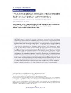
Distance sampling refers to a class of methods where the basic sampling unit is the sample point and information is obtained from distances to the nearest events, e.g., the first and second nearest events from the sampled points. The distribution of these distances under several spatial point processes generating the point pattern determines the performance of statistical tests and estimation procedures. The T 2 method, proposed by Besag and Gleaves (1973), generates powerful tests in the class of distance methods, as well as their modifications suggested by Hines and Hines (1979). Most of the distance sampling methods are based on the random selection of m points with uniform distribution in a sampling frame S lying slightly within the region A in order to avoid edge effects. Some distance methods can be based on systematic samples of m points, rather than random samples. In this paper, we consider only the situation where a random sample of points is used. Doguwa and Upton (1990) and Zimmerman (1991) have considered modifications on the distances to overcome edge effects in the context of parameter estimation, but their proposals have not been extended to hypothesis testing. In Figure 1, each dot represents an event as, for example, the position of a tree in a study region. Let O be the sample point and P and Q the first and second nearest neighbors of O, respectively. The event T is the nearest neighbor of P under the restriction that the angle OP T is equal to or larger than π/2. The T 2 method uses the squares of the distances OP and P T in the calculation of the test statistics. Denoting by ui , vi , and ti , for i = 1, . . . , m, the squares of the distances OP , P OQ, and P T , respectively, P and P zi = ui + ti /2, the test statistics are TN = (ui /zi )/m and TB = ui / zi . Under CSR and ignoring edge and overlap effects, TB has a beta distribution with parameters m and m, and TN has approximately a normal distribution with mean 1/2 and variance (12m)−1 (Diggle et al., 1976). Hines and Hines (1979) adapted the Eberhardt statistic (Eberhardt, 1967) by adding the T 2 information. The modified statistic is i (2ui + ti ) HI = 2m P √ √
2 , 2ui + ti i

P

for i = 1, . . . , m. The critical values for the complete spatial randomness test using the HI statistic is tabulated by Hines and Hines (1979). The power of the test modified by Hines and Hines is similar to those based on TN and TB , in the case of spatial regular patterns, and it is superior to them in the case of clustered alternatives (Hines and Hines, 1979). P The Pmethod proposed by Hopkins (1954) uses the test statistics H = ui / wi , where wi , i = 1, . . . , m, are the squared distances between m randomly selected events and their nearest neighbor events. This method is the most powerful among those proposed to test CSR. However, it is infeasible because random selection of events requires the complete mapping of events in the region. A proposal by Byth and Ripley (1980) would

Assun¸c˜ao and Reis: Testing spatial randomness

73

make this test feasible if certain subregions were completely mapped. We did not consider this distance measurement and quadrat mapping mixing approach in this paper. Hopkins’ test is used later on as a golden standard against which the other proposals can be contrasted.

o T o

H o o

o P o

o

G

O o o Q

o

o

o

o

o

Figure 1 Distribution of trees in a region. O is a randomly selected point, P is its nearest event, Q, G, and H are the second, third, and fourth nearest events, respectively, and T is the T-square nearest neighbor of P. In the next section, we review the angle-based test proposed by Assun¸c˜ ao (1994) and we introduce modifications to improve its power. The objective of this paper is to study the performance of tests using distance sampling data and angle-based tests. We take into account the field effort in the comparison between the tests by considering the total search area for events in each one of the tests.

2

The Angle Test and its Modifications

The angle test proposed by Assun¸c˜ ao (1994) is based on the smallest angle, denoted by θ, between the two vectors joining the sample point and its

74

Brazilian Journal of Probability and Statistics, 14, 2000

nearest and second nearest events. This angle is represented by POQ in Figure 1. Under CSR, θ is uniformly distributed in (0, π). With clustered patterns, the angle will tend to be smaller than expected under CSR. The explanation is that sample points outside clusters will typically produce small angles since the vectors should be pointing to the nearest cluster. With regular patterns, the angle will tend to be larger than expected under CSR, as is easy to see in the extreme case of a lattice. When m points are sampled in S, they generate the angles θ1 , . . . , θm measured at each point. With n events in the region, the sample intensity is defined as m/n. If the sample intensity is not larger than 10%, the angles can be considered independent (Diggle et al., 1976). Hence, under CSR, the angles θ1 , . . . , θm are approximately independent and with common distribution U (0,√π). The CSR hypothesis is tested using Kolmogorov’s test statistic d = m supx |Fm (x) − F (x)|, where Fm is the empirical distribution function and F (x) = x/π for x in (0, π). For tests with asymptotic levels 0.05 and 0.01, the critical values for comparison with d are 1.358 and 1.628, respectively. Compared with the T 2 tests, the angle test has comparable power when the configuration is characterized by events aggregated in small clusters. In less aggregated patterns, the angle test has somewhat smaller power but it should be noted that none of the T 2 tests is uniformly more powerful than the angle test. In regular patterns, the power of the angle test is comparable to that of TN and it is greater than TB (Assun¸c˜ ao, 1994). We suggest a modification of the angle test incorporating the information provided by the third and fourth nearest neighbor events of each sample point. In Figure 1, they are represented by G and H, respectively. The two additional events generate two tests. The first uses the previously defined θ and θt , the angle between the first and third nearest neighbor events (P OG angle). The second test uses θ, θt , and θf , the angle between the first and fourth nearest neighbor events (P OH angle). Like θ, the angles θt and θf are uniformly distributed in [0, π] and they are independent under CSR. In fact, conditioning on O and the fourth nearest event H, the three events within the disk of center O and radius OH are uniformly and independently distributed. Hence, θt and θf each have a uniform distribution in [0, π] and are independent. In this way, in the case of the first test, for each sample point, we have two angle measurements, yielding a total of 2m angles. Since these angles are approximately independent and identically distributed as U (0, π), the situation is equivalent to the original angle test with a sample twice as large and hence, we can use Kolmogorov’s d test statistic. The argument is analogous for the second test implying a sample three times larger than the number of sample points. Under the alternative hypothesis of aggregated or regular patterns, the angles θ, θt , and θf will tend to be smaller or larger than an observation with a distribution uniform on (0, π), respectively. In the case of clustered alternatives, this is due to the tendency of a sample point O to be outside

Assun¸c˜ao and Reis: Testing spatial randomness

75

clusters and its nearest neighbors to come out of a single cluster. As with the regular case, the second and third nearest neighbors will tend to be outside a neighborhood of the nearest neighbor P due to the regular pattern. Following a referee’s suggestion, we considered other tests for the uniform distribution different from the Kolmogorov test among those studied by Miller and Quesenberry (1979). We focused our attention on the Neyman Smooth Tests, the best tests found in their comparison. In particular, we considered the tests p22 and p24 defined as: 

2

k n X 1X  πr (Yj ) , p2k = n r=1 j=1

where π0 (Y ) = 1 √ π1 (Y ) = 12(Y − 0.5)  √  5 6(Y − 0.5)2 − 0.5 π2 (Y ) =  √  π3 (Y ) = 7 20(Y − 0.5)3 − 3(Y − 0.5)

π4 (Y ) = 210(Y − 0.5)4 − 45(Y − 0.5)2 + 9/8, where the Y ’s are random variables assuming values in the interval (0, 1). The use of angles and the possible increase in the information carried by the sample are particularly interesting if a ecologist is working in regions of difficult mobility. In these situations, the distance measurements would be time-consuming or expensive, while the angles could be easily obtained if the four nearest events can be identified at a distance. We note another advantage of the angle test compared to distance methods when the trees are located in slopes. In this case, it is not clear whether the bird’s-eye distance or the walking distance between trees should be used. The angle test does not suffer from this ambiguity.

3

Simulations

The power of the tests were obtained through Monte Carlo simulation of two types of point processes. The aggregated patterns were generated according to the Thomas modified process in A = [0, 50] × [0, 50] and S = [5, 45] × [5, 45] (Diggle et al., 1976). Initially, the parent events are distributed randomly in the study region according to a homogeneous Poisson process with density λ per unit area. Next, each parent event independently produces a random number of children events according to a Poisson distribution with mean µ. The position of each child event is determined by adding to the parent location a bivariate normal vector composed of

76

Brazilian Journal of Probability and Statistics, 14, 2000

independent variables with mean zero and variance σ 2 . In our simulations, we set λ = 0.2 and vary µ and σ. When we increase the value of µ, the number of events in each cluster increases. Decreasing σ will increase the degree of clustering of the children events around their parents. Processes with regular patterns were generated according to a Strauss process (Strauss, 1975). This process has a parameter r called inhibition radius, and two events located at x and y are considered neighbors if their distance is smaller than r. The conditional density of the locations, given that there are n events in A, depends only on the number of neighbors and it is given by (3.1) f (x1 , . . . , xn ; r) = α ρs , where α > 0, 0 ≤ ρ ≤ 1, and s is the number of distinct pairs of neighbors in x1 , . . . , xn . The parameter α is a normalizing constant and ρ reflects the inhibition degree of the process. The case ρ = 1 gives a Poisson process. For 0 < ρ < 1 fixed, the density of Strauss process stimulates the occurrence of patterns with a small number s of neighbors. In the limit, ρ = 0 produces a pattern where no two events in the region can be less than r units apart. We note that the parameter r does not appear explicitly in the density expression but it is implicitly used to calculate s. The events of the Strauss process were generated in A = [0, 70] × [0, 70] and S was chosen as [10, 60] × [10, 60]. The number of events was fixed as 200 and the radius of inhibition was 4. The parameter ρ varied from 0.0 to 0.8. The smaller this parameter, the stronger the regularity of the events’ configuration. For each value of the parameters, we generated 500 realizations of the processes considered. In each realization of the clustered processes, 25 sample points were chosen independently in S according to a uniform distribution. For the regular case, 15 sample points were chosen. The sample sizes were chosen to keep the sample intensity smaller than 10% guaranteeing that observations from different sample points can be considered independent (Diggle et al., 1976). The test statistics calculated were: three angle statistics with Kolmogorov test using one, two, and three angles (A, A3, A4, respectively), three angle statistics with Neyman’s p22 (AN 2, A3N 2, A4N 2, using one, two, and three angles, respectively) and Neyman’s p24 (AN 4, A3N 4, A4N 4, using one, two, and three angles, respectively). We also calculated the statistics of Hines and Hines (HI), Hopkins (H), TN , and TB . Given the number of realizations, the power β of theptests has asymptotic confidence interval with half-length equal to 1.96 ∗ β(1 − β)/500 ≤ 0.044. We set the significance level equal to 0.05. In the next subsections, we present the results of our simulations. Initially, in Section 3.1, we consider only the angle tests. In Section 3.2, we present the comparison of the best angle tests with those distance-based tests proposed previously in the literature. Finally, in Section 3.3, we compare the tests taking into account the field effort as a measure of cost.

Assun¸c˜ao and Reis: Testing spatial randomness

3.1

77

The power of the angle tests

80

100

Considering only the Neyman statistics, the angle tests using p22(AN 2,A3N 2, A4N 2) had an uniformly greater power than tests using p24 , both in regular patterns and in clustered patterns (results not shown but available from the authors upon request). Therefore, we consider only p22 tests from now on.

0

20

40

power(%)

60

AN2 A3N2 A4N2 A A3 A4

0.0

0.2

0.4

0.6

0.8

rho

Figure 2(a) Angle tests power against spatial regular alternatives. The tests A, A3, and A4 use the Kolmogorov statistic and the numbers on the tests’ labels indicate the number of additional neighbor angles collected around the sample point. The tests AN 2, A3N 2, and A4N 2 are similar but use the p22 Neyman’s statistic instead. Figure 2(a) shows the results for angle tests using p22 and the Kolmogorov-based tests in the situation of regular patterns. We can see that the p22 statistics has greater power than their equivalent tests using Kolmogorov

78

Brazilian Journal of Probability and Statistics, 14, 2000

statistics. Furthermore, the modified angle tests with third nearest neighbor information (A3, and A3N 2) add power to the originally proposed angle test (A, and AN 2, respectively). For ρ < 0.2 (very regular patterns), the angle using the fourth nearest neighbor is usually not greater than the expected under CSR and, in fact, it tends to be smaller than under CSR. Also, by adding the fourth nearest neighbor angle to the A3 and A3N 2 tests reduces the power of the resulting tests A4 and A4N 2, respectively. Furthermore, for ρ > 0.2, the addition of the fourth nearest neighbor does not increase the power significantly.

2.0

100 2.5

80 3.0

0.5

1.0

1.5

2.0

mu

mu

sigma=0.50

sigma=0.60

3.0

8

10

8

10

power(%)

60

80

2.5

0

20

40

80 60 40 0

20

4

6

8

10

2

4

6 Mu

sigma=0.75

sigma=1.0

60 20 0

0

20

40

power(%)

60

80

100

Mu

80

100

2

40

power(%)

60 0

1.5

100

1.0

100

0.5

power(%)

sigma=0.40

20

power(%)

60 40 0

20

power(%)

80

AN2 A3N2 A4N2 A A3 A4

40

100

sigma=0.25

2

4

6 Mu

8

10

2

4

6 Mu

Figure 2(b) Angle tests power against spatial clustered alternatives. Tests A, A3, and A4 use the Kolmogorov statistic and the numbers on the tests’ labels indicate the number of additional neighbor angles collected around the sample point. Tests AN 2, A3N 2, and A4N 2 are similar but use the p22 Neyman’s statistic instead. Figure 2(b) makes the same comparison in the situation of clustered alternatives. Analyzing these graphs, we observe three aspects: (1) once

Assun¸c˜ao and Reis: Testing spatial randomness

79

again, the angle tests using the statistic p22 have better performance than the angle tests using Kolmogorov statistic; (2) the tests using information on the third and fourth nearest neighbor increased the power of the originally proposed angle test; (3) generally, tests using fourth nearest neighbor information (A4 and A4N 2) are better than those with information up to the third nearest neighbor, except for the case of patterns with high degree of clustering and very tight clusters (σ = 0.25 and 0.40 with µ ≤ 1.5). The above exception can be explained by the small size of the clusters. Let X be the number of children generated by a single parent event and assume X has a Poisson distribution with mean µ. If µ ≤ 2, then the clusters have few events since P (X < 4) ≥ 0.86. This implies that, with high probability, the third and fourth nearest neighbors are from clusters different from those of the first and second nearest neighbors. Hence, the angles associated with the farthest neighbors tend to be larger than if they come from the same cluster. The three aspects listed above can be easily recognized by examining of the pairs of lines (A and AN 2, A3 and A3N 2, A4 and A4N 2) in the graphs for σ = 0.50 and σ = 0.60. Considering the information provided by Figures 2(a) and 2(b), we decided to present the rest of the comparisons using only the angle tests with the Neyman p22 statistic (AN 2, A3N 2, and A4N 2), since these are better than its p24 counterparts.

3.2

Comparison with distance-based tests

Figure 3(a) shows the power of Hopkins, Hines and Hines, TN , and the angle tests (original and modified) in the situation of regular patterns. We observe that Hopkins test has the greatest power followed by the Hines and Hines test for very regular patterns (ρ = 0.0 and ρ = 0.2). As the regularity decreases (i.e., ρ increases), these two tests have similar power. The original angle test power is slightly smaller than that of TN and, by adding the third nearest neighbor angle information, it becomes comparable to TN . When ρ increases, the tests TN , AN 2, and A3N 2 are very similar. The power of TB is very small and it is not shown here. Notice that all tests lose much of their power when ρ increases. In Figure 3(b), we show the results for aggregated patterns, according to the values of the parameters σ and µ. The tests of Hopkins and Hines and Hines are uniformly most powerful among the tests and they are very similar except when the pattern is less clustered and with larger clusters (σ = 0.75 and µ > 5.0; σ = 0.1 and µ > 1.0). In this case, the Hines and Hines test is clearly better than the Hopkins test. As noted in Assun¸c˜ ao (1994), there is not a uniformly more powerful test among the tests TN and TB in the case of clustered alternatives. If σ < 0.5, the first test is the best one, while the latter is the best one if σ ≥ 0.5. This is clearly a disadvantage of these tests since it is not possible to decide which one should be used without knowing the value of the parameter. Comparing the angle tests with the TN and TB tests, we note that A4N 2 has power

80

Brazilian Journal of Probability and Statistics, 14, 2000

80

100

similar to the best between TN and TB for patterns with high clustering degree.

0

20

40

power(%)

60

Hopkins TN Hines AN2 A3N2 A4N2

0.0

0.2

0.4

0.6

0.8

rho

Figure 3(a) Power of the tests proposed by Hopkins, Hines and Hines, TN and angle tests against spatial clustered alternatives.

3.3

Comparing power taking sampling effort into account

In any field work, each sampling procedure implies specific costs. Therefore, a comparison between sampling schemes to collect CSR testing data should take these costs into account. It is important to know the relationship between the sampling effort and the power of a test because a given test can have great power but at a high cost while another test can have power somewhat smaller than the first test with low cost. In the case of the angle tests, by considering additional nearest neighbor angles, we increase field effort which could be employed to sample more points. The latter alternative has more sampling points when compared to the first one. However, it collects information on the first two nearest neighbors angle only, while the first sampling method collects information

Assun¸c˜ao and Reis: Testing spatial randomness

81

on the first four nearest neighbors giving more information at each sampling point. It is not clear which of these procedures is preferable.

1.5

2.0

100 2.5

80 3.0

0.5

1.0

1.5

2.0 mu

sigma=0.50

sigma=0.60

2.5

3.0

8

10

8

10

60 40 0

0

20

40

60

power(%)

80

100

mu

80

100

1.0

20

4

6

8

10

2

4

6 Mu

sigma=0.75

sigma=1.0

60 20 0

0

20

40

60

power(%)

80

100

Mu

80

100

2

40

power(%)

60 0

20

power(%)

60 40 0

20

power(%)

80

Hopkins T2 Hines AN2 A3N2 A4N2

0.5

power(%)

sigma=0.40

40

100

sigma=0.25

2

4

6 Mu

8

10

2

4

6 Mu

Figure 3(b) Power of the tests proposed by Hopkins, Hines and Hines, TN and angle tests against spatial regular alternatives. For σ = 0.25 and 0.40, the test T 2 is based on the TN statistic. For the other values of σ, the test is based on TB . Although highly desirable, general measures of cost are not simple to devise. The cost of a sampling procedure is highly variable depending on many aspects specific to a particular application. In particular, the difficulty of movement accross the terrain and the cost of a measurement (angle or distance) are major components in the sampling effort of a study and they are quite different among applications. To work with a general measure of cost of a sampling method, we consider the total search area necessary to obtain the information. Although crude, this measure gives some idea of field effort needed to apply the method of data collection. In this section, we compare the power of different sampling procedures taking into account the cost represented by the total search area to get

82

Brazilian Journal of Probability and Statistics, 14, 2000

20

the data. We studied the methods HI, TN , TB , A3N 2, A4N 2, and the originally proposed angle test with more sampling points. One approach to include the cost information would be to compare the power of tests with the constraint of equal sampling costs. Since the search area of our tests is a random variable, we could work with the expected search area. However, there is no closed form expression for this search area under our alternative hypothesis models which leads us to work with the average over the simulations, as explained below.

10 0

5

power(%)/area

15

Hines TN AN2 A3N2 A4N2 A2.0N2 A3.0N2

0.0

0.2

0.4

0.6

0.8

rho

Figure 4(a) Performance (power (%)/ search area) in the case of regular alternatives. The tests A2.0N 2 and A3.0N 2 correspond to the angle test AN 2 using 2 and 3 times more sample points, respectively, than the other tests. We carried out additional simulations to address the issue of cost. In both cases, aggregated and regular, we kept the same parameter values as before. In the regular case, we generated 150 events by the Strauss process in a square region with side equal to 50 using inhibition radius equal to 3. We sampled 15 points in each of 500 independent simulations for each

Assun¸c˜ao and Reis: Testing spatial randomness

83

parameter value. The aggregated case also considered 500 independent simulations for each parameter value and sampled 25 points. We used the angle test as proposed by Assun¸c˜ ao (1994) with sample points sizes 1.5, 2, 2.5, and 3 times larger than the sample points size used for the modified angle tests A3N 2 and A4N 2 and for the Hopkins test. In the figures, we show only the original angle tests using two and three times more sample points and they are denoted by A2.0N 2 and A3.0N 2, respectively. Note that, under the CSR null hypothesis, A3N 2 and A2.0N 2 have the same sample size and the same distribution if the different sample points generate independent information. In a single simulation, the total search area of an angle test is calculated as the sum of the search areas in each sample point, represented by the circle area centered at the sample point with radius equal to the distance between the sample point and its farthest neighbor used in the test. In the Figure 1, for example, for the AN 2 test the circle radius is the distance between the sample point (O) and its second nearest neighbor (Q) while, for the A3N 2 test, the third nearest neighbor (G) is used. For the T 2 tests, the search area in each sample point is calculated as the sum of the circle area centered at the sample point and radius equal to the distance between the sample point and its first nearest neighbor (P) and the half circle area centered at the first nearest neighbor (P) and radius equal to the distance between this neighbor and its T 2 neighbor (T). Then, we obtain the average of the total search area over all 500 simulations for each parameter value and for each test procedure. The results for the regular case are in Figure 4(a). For all parameter values, Hines and Hines’ test is the best one and its performance, as measured by the ratio power(%)/area, is approximately 50% greater than that of the second best test. This second best is the TN , which is superseded by AN 2 only when ρ = 0. In this case of extreme regularity, represented in the simulations by ρ = 0, the tests A3N 2 and A2.0N 2, which have equal sample sizes but different distributions under the alternatives, have very similar performances measured as power(%)/area. Test A3.0N 2 is better than test A4N 2 due to the low power of the latter which was mentioned earlier. In situations of moderate regularity (ρ = 0.2, 0.4, 0.6), the relationship cost-benefit of all tests substantially decreases. When there is little regularity, the performances of the tests are approximately the same and very low. The results for the aggregated case are depicted in the Figure 4(b). Once again, in all situations, Hines and Hines’ test presents better performance than all other competitors. This performance increases with σ and µ. In second place, we have one of the T 2 tests but which one is best depends on parameter values. For σ = 0.25 and 0.40, the test T 2 is that based on the TN statistic. For the other values of σ, the test is that based on TB . In all situations considered, the A3N 2 and A4N 2 modified angle tests are better than their equivalents A2.0N 2 and A3.0N 2, respectively. The modified angle tests present a cost-benefit relationship very similar, especially if the degree of clustering is extreme (σ = 0.25 and σ = 0.40),

84

Brazilian Journal of Probability and Statistics, 14, 2000

but, when the degree of clustering is small (σ = 1.0), all angle tests are equivalent.

2.0

2.5 2.5

2.0 3.0

0.5

1.0

1.5

2.0

mu

mu

sigma=0.50

sigma=0.60

3.0

8

10

8

10

1.5

2.0

2.5

0.0

0.5

1.0

power(%)/area

2.0 1.5 1.0 0.0

0.5

4

6

8

10

2

4

6 Mu

sigma=0.75

sigma=1.0

1.5 0.5 0.0

0.0

0.5

1.0

1.5

power(%)/area

2.0

2.5

Mu

2.0

2.5

2

1.0

power(%)/area

1.5 0.0

1.5

2.5

1.0

2.5

0.5

power(%)/area

sigma=0.40

0.5

power(%)/area

1.5 1.0 0.0

0.5

power(%)/area

2.0

Hines T2 AN2 A3N2 A4N2 A2.0N2 A3.0N2

1.0

2.5

sigma=0.25

2

4

6 Mu

8

10

2

4

6 Mu

Figure 4(b) Performance (power (%)/ search area) in the case of clustered alternatives. The tests A2.0N 2 and A3.0N 2 correspond to the angle test AN 2 using 2 and 3 times more sample points, respectively, than the other tests. For σ = 0.25 and 0.40, the test T 2 is based on the TN statistic. For the other values of σ, the test is based on TB .

4

Conclusions

Although we cannot cover all possibilities for spatial pattern in our simulations, the results enable some appreciation of how the tests behave. The Hines and Hines test emerges as the best test among those considered in this paper. It is the most powerful and has better performance than its competitors. The T 2 test has smaller power but there is one additional

Assun¸c˜ao and Reis: Testing spatial randomness

85

problem with this proposal: the best test among TN or TB will depend on the true, but unknown, spatial pattern of events. The information added to the angle test by the third and fourth nearest neighbors increased the power of the test to detect aggregated and regular patterns. The test based on the three angles has power comparable to the best among TN and TB . These angle tests would not require additional sampling effort if the four nearest events can be identified at a distance. Particularly, when the T-square neighbors are not one of four nearest neighbors, the angle test can save the sampling effort of searching for the T-square neighbor. However, this last situation is not very likely to occur frequently. Sampling more points in the region increases the original angle test power by a larger amount than collecting additional angle information around sample points. However, in the more realistic situations of moderate clustering or regularity this increase in power is not large. In these cases, if the terrain makes distance measurements difficult, it can compensate to locally sample more spatial information rather than to walk large distances between sample points. Hence, in problems where the angle measurements can be done easily and when the three angle measurements are less costly than distance measurements, angle test A4 can be a viable alternative to test the complete spatial randomness hypothesis.

Acknowledgements We are grateful to FAPEMIG, FINEP and CNPq, Brazilian research foundations, for partial support of our research. We thank Julian Besag for comments which eventually led to this paper and Stephen Perz and Mauro Costa for his help in improving the readability of the text. We also thank an anonymous referee for suggestions that improved the paper. Received February, 1999. Revised May, 2000.)

References Assun¸c˜ ao , R.M. (1994). Testing spatial randomness by means of angles. Biometrics, 50, 531–537. Besag, J.E. and Gleaves, J.T. (1973). On the detection of spatial pattern in plant communities. Bull. Int. Statist. Inst., 45, 153–158. Byth, K. and Ripley, B.D. (1980). On sampling spatial patterns by distance methods. Biometrics, 36, 279–284.

86

Brazilian Journal of Probability and Statistics, 14, 2000

Diggle, P.J., Besag, J.E. and Gleaves, J.T. (1976). Statistical analysis of spatial point patterns by means of distance methods. Biometrics, 32, 659–667. Diggle, P.J. (1983). Statistical analysis of spatial point patterns. London: Academic Press. Doguwa, S.I., Upton, G.J.G. (1990). On the estimation of the nearest neighbor distribution, G(t), for point processes. Biometrical Journal, 32, 863–876. Eberhardt, L.L. (1967). Some developments in distance sampling. Biometrics, 23, 207–216. Hines, W.G.S. and Hines, R.J.O. (1979). The Eberhardt index and the detection of non-randomness of spatial point distributions. Biometrika, 66, 73–80. Hopkins, B. (1954). A new method of determining the type of distribution of plant individuals. Annals of Botany, 18, 213–227. Miller Jr., F.L., Quesenberry, C.P. (1979). Power studies of tests for uniformity, II. Communications in Statistics - Simulation and Computation, B, 8, 271–290. Strauss, D.J. (1975). A model for clustering. Biometrika, 62, 467–475. Zimmerman, D. (1991). Censored distance-based intensity estimation of spatial point processes. Biometrika, 78, 287–294.