Testing the gravity p-median model empirically Authors: Kenneth Carling, Mengjie Han, Johan Håkansson, and Pascal Rebreyend This version: 2015-06-08
Kenneth Carling is a professor in Statistics, Mengjie Han is a PhD in Micro-data analysis, Johan Håkansson is a professor in Human Geography, and Pascal Rebreyend is a professor in Computer Science at the School of Technology and Business Studies, Dalarna university, SE-791 88 Falun, Sweden. Corresponding author. E-mail:
[email protected]. Phone: +46-23-778573. -1-
Abstract: Regarding the location of a facility, the presumption in the widely used p-median model is that the customer opts for the shortest route to the nearest facility. However, this assumption is problematic on free markets since the customer is presumed to gravitate to a facility by the distance to and the attractiveness of it. The recently introduced gravity p-median model offers an extension to the p-median model that account for this. The model is therefore potentially interesting, although it has not yet been implemented and tested empirically. In this paper, we have implemented the model in an empirical problem of locating vehicle inspections, locksmiths, and retail stores of vehicle spare-parts for the purpose of investigating its superiority to the p-median model. We found, however, the gravity p-median model to be of limited use for the problem of locating facilities as it either gives solutions similar to the p-median model, or it gives unstable solutions due to a non-concave objective function. Key words: p-median model, distance decay, market share, network, retail, simulated annealing, travel time
1. Introduction The general problem of allocating P facilities to a population geographically distributed in Q demand points remains as an important research and applied issue. The precursor Hakimi considered the task of locating telephone switching centers and formalized what is now known as the p-median model. The p-median model addresses the problem of allocating P facilities to a population geographically distributed in Q demand points such that the population’s average or total distance in a network to its nearest facility is minimized (e.g. Hakimi 1964, Handler and Mirchandani 1979, and Mirchandani 1990). After Hakimi’s work, the p-median model has been used in a remarkable variety of location problems (see Hale and Moberg, 2003). However, it has been argued that the p-median model is inappropriate for locating facilities in a competitive environment because of the assumption that customers opt for the nearest facility (see e.g. Hodgson, 1978 and Berman and Krass, 1998). Location studies on competitive environments have predominately considered market areas with already existing facilities competing for customers. These models are designed for estimating -2-
market shares and are based on the gravity model as presented by Huff (1964, 1966). To describe the customers’ spatial choice behavior, he proposed that the probability of a customer patronizing a certain facility is to be modelled as a function of distance to and attractiveness of the facility. This model specifies for each customer a probability distribution of patronage for each facility in the market area. Thereby, the market share of a facility might be evaluated by aggregating all the customers and corresponding probabilities in the area of interest. The same behavioral model has been used for investigating the effect of adding or removing a single facility in the market area contingent to a specific location of that facility (see Lea and Menger, 1990). Moreover, an optimal location with regard to some desirable outcomes may be identified (Holmberg and Jornsten, 1996). However, the customers’ spatial choice behavior has not been invoked in the general facility location problem addressed by the p-median model, until recently. Drezner and Drezner (2007) presented the gravity p-median model that integrates the gravity rule with the p-median model. In their paper, they restate arguments for the gravity rule that can be found elsewhere: 1) the population is often spatially aggregated and approximately represented by the center of the demand point, 2) customers might act on incomplete information regarding the distance to each of the facilities, and 3) facilities vary in attractiveness to customers. There is also a fourth argument namely that the choice of facility may depend on other purposes for a trip (Carling and Håkansson, 2013). Up to now, the computational aspects of the gravity p-median model using synthetic data have been in focus with the intention of finding good solutions to the NP-hard problem (Drezner and Drezner, 2007 and Iyiguna and Ben-Israel, 2010).1 To the best of our knowledge, the gravity p-median model has never been applied on real data. The aim of this paper is therefore to investigate the supposed superiority of the gravity p-median model over the classical p-median model in competitive environments in real world location problems. In the empirical test we consider three cases with P small, in a Swedish region where the customers
1
The same holds for Drezner and Drezner’s (2011) extension of the model to a multiple server location problem. -3-
are geo-coded and details of the network is available. The cases are selected so as to represent markets where customers’ spatial choice behavior ranges from distance minimizing to the gravity rule. The first case is the location of vehicle inspections where the behavioral assumption of the p-median model is expected to be appropriate. The third case is retail stores of vehicle spare-parts where the gravity rule is expected to apply. The second case is locksmiths where the market situation is ambiguous with regard to the applicability of the gravity rule. In the analysis, we compare the current location of facilities in these three cases to the gravity p-median and p-median solutions. This paper is organized as follows: section two presents the empirical setting and gives the implementation of the models. Section three presents the results of the empirical test of the gravity p-median model benchmarked by the classical p-median model and the current market solution. The fourth section concludes the paper with a discussion.
2. Settings of the empirical test To enable an investigation of the supposed superiority of the gravity p-median model over the p-median model in a competitive environment, a setting is required that allows for real world application of the models where the validity of the gravity rule can be assessed beforehand. In this section we provide geographical information about the markets, the implementation of the models, and the business cases used in the empirical test. 2.1 Geography Figure 1 shows the Dalecarlia region in central Sweden, about 300 km northwest of Stockholm. The size of the region is approximately 31,000 km2. Figure 1a depicts the location of customers in the region2. As of December 2010, the Dalecarlia population numbers 277,000 residents. About 65 % of the population lives in 30 towns and villages of between 1,000 and 40,000 residents, whereas the remaining third of the population resides in small, scattered settlements. Figure 1b shows the landscape and it gives a perception of the geographical distribution of the 2
The population data used in this study comes from Statistics Sweden, and is from 2002 (www.scb.se). The residents are registered at points 250 meters apart in four directions (north, west, south, and east) implying a maximum error of 175 meters in the geo-coding of the customers. There are 15,729 points that contain at least one resident in the region. -4-
population. The altitude of the region varies substantially; for instance in the western areas, the altitude exceeds 1,000 meters above sea level whereas the altitude is less than 100 meters in the southeast corner. Altitude variations, the rivers’ extensions, and the locations of the lakes provide many natural barriers to where people could settle and how a road network could be constructed in the region. The majority of residents live in the southeast corner while the remaining residents are located primarily along the two rivers and around Lake Siljan in the middle of the region. The region constitutes a secluded market area as it is surrounded by extensive forest and mountain areas which are very sparsely populated. Hence, in the following we ignore potential influence of customers and facilities outside the region. 2.2 Distance measure Carling, Han, and Håkansson (2012) and Carling, Han, Håkansson, and Rebreyend (2015) found the Euclidian distance measure to perform poorly for the p-median problem, leading to suboptimal locations and biased market shares in this rural area. In the empirical analysis we have tested the Euclidean measure but because of its shortcomings we focus in what follows on the travel-time distance. To obtain the travel-time, we assumed that the attained velocity corresponded to the speed limit on the road network. The Swedish road system is divided into national roads and local streets which are public as well as subsidized and non-subsidized private roads. In Dalecarlia, the total length of the road system in the region is 39,452 km (see Figure 1d).3, Rebreyend, Han, and Håkansson (2014) used the p-median model on this road network, and they noted that for P small the national road network was sufficient. Therefore, we only use the national roads in this study. Figure 1c shows the national road network in the region. The national road system in the region totals 5,437 km with roads of varying quality which are in practice distinguished by a speed limit. The speed limit of 70 km/h is default and the national roads usually have a speed limit of 70 km/h or more. 3
The road network is provided by the NVDB (The National Road Data Base). The NVDB was formed in 1996 on behalf of the government and is now operated by the Swedish Transport Agency. NVDB is divided into national roads, local roads and streets. The national roads are owned by the national public authorities, and their construction is funded by a state tax. The local roads or streets are built and owned by private persons, companies, or by the municipalities. Data was extracted in spring 2011 and represents the network of winter 2011. The computer model is built up by about 1.5 million nodes and 1,964,801 road segments. -5-
Figure 1: Map of the Dalecarlia region showing (a) one-by-one kilometer cells where the population exceeds 5 inhabitants, (b) landscape, (c) national road system, and (d) national road system with local streets and subsidized private roads.
2.3 Objective functions, variables, and parameters The objective of both the p-median model and gravity p-median model is to locate P facilities to a -6-
population geographically distributed in Q demand points. We will use the following notations. N is the number of nodes, q and p indexes the demand and the facility nodes respectively, wq the demand at node q, and d qp the shortest distance between the nodes q and p. Further, for the p-median model is important to note that Hakimi (1964) showed that the optimal solution of the p-median model exists at the network’s nodes. The objective function for the p-median model is ∑𝑞∈𝑁 𝑤𝑞 min𝑝∈𝑃 {𝑑𝑞𝑝 }. The objective function for the gravity p-median model is similar with the addition of a term specifying the probability that a customer located at node q will visit a facility at node p. Drezner and Drezner (2007) specify the probability term as
𝐴𝑝 𝑒 −𝜆𝑑𝑞𝑝 ∑𝑝∈𝑃 𝐴𝑝 𝑒 −𝜆𝑑𝑞𝑝
, where 𝐴𝑝 denotes the attractiveness of the facility and 𝜆
denotes the parameter of the exponential distance decay function4. As a consequence, the objective function of the gravity p-median model is min𝑝∈𝑃 {∑𝑞∈𝑁 [𝑤𝑞
∑𝑝∈𝑃 𝑑𝑞𝑝 𝐴𝑝 𝑒 −𝜆𝑑𝑞𝑝 ∑𝑝∈𝑃 𝐴𝑝 𝑒 −𝜆𝑑𝑞𝑝
]}.
As noted above, we use travel-time as the distance measure which means that the quickest path between q and p needs to be identified. We implemented the Dijkstra algorithm (Dijkstra 1959) and retrieved the shortest travel time from the facilities to residents in each evaluation of the objective function. We imposed that facilities are located at the nodes of the network even though the Hakimi-property does not generally apply to the gravity p-median model (Drezner and Drezner, 2007). The reason for this choice is to enable a fair comparison with the p-median solutions which will be at the nodes. Moreover, all customers are assigned to the facilities which means that we abstract from the possibility of lost demand, i.e. the case when some customers seek substitutes because of the facilities being inaccessible for them (Drezner and Drezner, 2012). The parameter, 𝐴𝑝 , is supposed to represent the attractiveness to the customers of the facility and, in the extensive literature in market research on the topic, it is for instance measured as the facility’s floor area (Huff, 1966). The value of lambda5 is related to the spatial behavior of the customer and decisive on how far she 4
The exponential function and the inverse distance function dominate in the literature as discussed by Drezner (2006). The solutions to the location models are obtained in the travel time network. To conform to the existing literature, we discuss lambda in terms of a parameter for a road network. In the algorithm we adjust lambda to the corresponding value in the travel time -75
is likely to travel for patronizing a facility. For λ=0, all (equally attractive) facilities are equally likely to be patronized by the customer, irrespective of the customer’s distance to them. The larger the value of lambda, the more attached the customer is to the nearest facility. Drezner (2006) derived λ=0.245 for shopping malls in California whereas Huff (1964, 1966) reported, albeit using the inverse distance function, on larger values of λ for grocery and clothing stores. We use Drezner’s value converted from Euclidean distance and English miles into the corresponding value for the network distance and in kilometers. By assuming the network distance 6 to be 1.3 times the Euclidean distance we have λ=0.11, which means that average travel to patronize a facility equals 9 kilometers. Table 1: Swedes self-estimated network distance for purchases of durable goods. Travel distance (km) Proportion (%)
250
14
22
32
17
9
4
2
A value of lambda specific for the applications here is λ=0.035, which means that average travel to patronize a facility is about 30 kilometers. We obtained this value as the maximum likelihood estimate of the parameter based on grouped data from the Swedish Trade Federation (Svensk Handel). The data values are shown in Table 1. In the empirical part, we only consider goods and services requiring infrequent trips which ought to be like durables. 2.4 Implementation of simulated annealing The p-median problem is NP-hard (Kariv and Hakimi, 1979) and so is the gravity p-median problem. Rebreyend et al (2014) discussed and examined solutions to the p-median problem for the region’s network. They advocated the simulated annealing algorithm which is used here and also used for the gravity p-median model.7 This randomized algorithm is chosen due to its ease of implementation and the quality of results regarding complex problems. Most important in our case is that the cost of evaluating a solution is high and therefore we prefer an algorithm which keeps the number of evaluated solutions low (Kirkpatrick, Gelatt, and Vecchi, 1983). network. 6 Love and Morris (1972) found a coefficient of 1.78, however the relationship has been observed elsewhere in the literature and found relevant for this network in Carling et al (2012). 7 Drezner and Drezner (2007) discussed alternative heuristic algorithms, finding little difficulty in solving the problem with standard heuristics. -8-
The simulated annealing (SA) is a simple and well described meta-heuristic. Al-khedhairi (2008) describes the general SA heuristic procedures. SA starts with a random initial solution s, the initial temperature 𝑇0 , and the temperature counter 𝑡 = 0. The next step is to improve the initial solution. The counter 𝑛 = 0 is set and the operation is repeated until 𝑛 = 𝐿. A neighbourhood solution 𝑠 ′ is evaluated by randomly exchanging one facility in the current solution to the one not in the current solution. The difference, Δ, of the two values of the objective function is evaluated. We replace s by 𝑠 ′ if Δ < 0, otherwise a random variable 𝑋 ∼ 𝑈(0,1) is generated. If 𝑋 < 𝑒 (
Δ⁄ ) 𝑇 ,
we still replace
s by 𝑠 ′ . The counter 𝑛 = 𝑛 + 1 is set whenever the replacement does not occur. Once 𝑛 reaches L, 𝑡 = 𝑡 + 1 is set and T is a decreasing function of t. The procedure stops when the stopping condition for t is reached. Table 2: Average value of the objective function as well as the lower bound of a 99% confidence interval for the minimum of the objective function (in parenthesis). Location model PM
GPM (λ=0.11)
GPM (λ=0.035)
Vehicle Insp.
611.09 (597.16)
794.06 (756.36)
1724.86 (1671.46)
Locksmiths
798.45 (778.91)
946.59 (907.23)
1756.08 (1713.88)
Spare-parts
545.80 (518.53)
745.23 (708.12)
1716.51 (1669.63)
na
754.57 (739.23)
1716.86 (1664.78)
na
757.89 (718.12)
1702.54 (1669.79)
Business
-
𝐴𝑝 fivefold 𝐴𝑝 twofold
The main drawback of the SA is the algorithm’s sensitivity to the parameter settings. To overcome the difficulty of setting efficient values for parameters such as temperature, an adaptive mechanism is used to detect frozen states and if warranted re-heat the system.8 In all experiments, the initial temperature was set at 400 and the algorithm stopped after 10,000 iterations. Each experiment was computed twice with different random starting points to reduce the risk of local solutions. To ascertain the quality of the solution we also applied a method for computing a 99% confidence interval for the minimum, to which the obtained solution can be compared. In doing so, we follow Carling and Meng (2015a, 2015b) and compute the statistical lower bound. Table 2 gives the average of the objective function obtained as a solution to its minimum as well as the statistical lower bound. The businesses under study are described in the ensuing subsection. 8
Our adaptive scheme to dynamically adjust temperature works as follow: after n=10 iterations with no improvement, the temperature is increased according to newtemp=temp*3^β, where β starts at 0.5 and is increased by 0.5 each time the system is reheated. As a result, the SA will never be in a frozen state for long. The temperature is decreased each iteration with a factor of 0.95. The settings above are a result of substantial preliminary testing on this data and problem. In fact, some of the solutions were compared to those obtained by alternative heuristics. -9-
Typically, the solutions are some 10 to 40 seconds away from a lower bound of the minimum which we consider sufficiently precise for this type of applications. 2.5 Businesses under study As mentioned above, the cases are selected to represent markets where the customers’ spatial behavior should be distinctly different. In the interest of visualizing the difference in model implied locations, it is desirable that the number of facilities in the market is small. We selected vehicle inspections, locksmiths, and retailers in vehicle spare parts. The problem of locating vehicle inspections appears frequently in the literature on the p-median model (see e.g. Francis and Lowe, 1992). In Sweden, vehicle inspection was a state monopoly until 2009 when the market was deregulated. A state monopoly may be clearly regarded as a central planner and we therefore expect current locations of the inspections to resemble the p-median solution. As of October 2012 there are eleven vehicle inspections operated by two companies in Dalecarlia. The inspections perform vehicle safety checks of vehicles according to EU protocol; hence there is no reason to expect the inspections to vary in attractiveness. Furthermore, the owner of a vehicle is required to regularly have the vehicle inspected. Older vehicles are subject to annual inspections whereas newer ones, inspections are triennial. Thus, a trip to the vehicle inspection is an infrequent patronage. There are seven locksmiths in the region. These are small business without any central control. The virtue of the business makes it far-fetched that locksmiths differ much in attractiveness. Putting these two facts together, it is difficult to decide whether to expect customers to locksmiths to comply with the gravity rule or not. The third business is retail stores of vehicle spare-parts. There are two competitors in the region. One has 12 facilities in the region and the other has 2 facilities. However, the stores of the latter competitor are large and offer an ample selection of spare-parts as well as many complementing products. We expect these two stores to be quite more attractive. We consider two assumptions. The first is the case where the two stores are twice as attractive as the competitor’s stores. The second is - 10 -
the case where the two stores are assumed to be five times as attractive.
3. Results In this section, we depict the current location of facilities in the three business cases. We also depict the solutions provided by the p-median model and gravity p-median model. For vehicle inspections, we do not believe the gravity rule to apply and therefore expect the p-median solution to mimic the current location and the gravity p-median solution to be inapt. However, we expect the gravity p-median solution to be superior in the case of vehicle spare parts retailers. We provide results for two levels of value on λ as well as three levels of attractiveness. We anticipate that the most reasonable values of the two parameters should be 0.035 and 5, respectively. We also provide results on the value of the objective function allowing for a comparison on the average travel-time for the model implied scenarios as well as results on the market area for the facilities.
Figure 2: Map of the Dalecarlia region showing the current locations and the p-median (PM) solution for (a) vehicle inspections and (b) locksmiths.
Figure 2 shows the current location of the 11 vehicle inspections (Figure 2a) and the 7 locksmiths (Figure 2b) in the region. Imposed on the map in the figure is the solution to the p-median model - 11 -
(hereafter PM) for the two businesses. As expected, the current location of the vehicle inspections is quite near to the PM solution where ten out of eleven facilities coincide. The current locations of the seven locksmiths differ from the PM solution, but not by much. We now turn to the gravity p-median model (hereafter referred to as GPM followed by λ used) and how it compares to PM. Figure 3 shows that the GPM(0.11) solution is similar to the PM solution; for the vehicle inspections problem, the results of the models coincides almost completely. The similarity is also apparent in the case of locksmiths.
Figure 3: Map of the Dalecarlia region showing the p-median (PM) solution and the gravity p-median (GPM) solution with 𝜆 = 0.11 for (a) vehicle inspections and (b) locksmiths.
To understand the practical difference between the solutions of the PM and the GPM(0.11) models, we compute the travel-time to the nearest facility for customers in the region. Table 3 shows the average travel-time to the current locations, the PM, and the GPM solutions. The GPM(0.11) gives solutions that imply some two per cent longer travel time to the nearest vehicle inspection or locksmiths compared to the PM solutions. Table 3 also gives the average travel-time for the GPM(0.035) solutions. Recall that this model is the best estimate of how Swedish customers patronize facilities of durable goods and services. The - 12 -
GPM(0.035) solutions differ substantially from the PM where the GPM(0.035) solutions imply some 50 per cent longer trips to the nearest facility on average. Table 3: The customers’ average travel-time (seconds) to the nearest facility for current locations and p-median (PM) as well as gravity p-median (GPM) solutions. Location model Business
Current
PM
GPM (λ=0.11)
GPM (λ=0.035)
Vehicle Insp.
612.65
611.09
629.59
863.77
Locksmiths
1014.36
798.45
815.92
1188.09
Spare-parts
789.94
545.80
551.97
808.19
na
na
588.29
823.73
na
na
583.83
897.11
-
𝐴𝑝 fivefold 𝐴𝑝 twofold
Following up on the findings in Table 3, Figure 4 contrasts the GPM(0.035) solutions to the PM solution for vehicle inspections (Figure 4a) and locksmiths (Figure 4b). The models provide distinctively different geographical configuration of locations. For the GPM(0.035), facilities tend to be clustered in some towns, and we stress that it is not because the algorithm entered local minima as we have tested several starting values and the clustering pattern repeated itself.
Figure 4 Map of the Dalecarlia region showing the p-median solution (PM) and the gravity p-median solution (GPM) with 𝜆 = 0.035 for (a) vehicle inspections and (b) locksmiths.
The clustering pattern indicates a difficulty to identify potential locations which give a unique - 13 -
market area for a facility. Consider that λ=0.035 implies that a customer’s expected travel distance is about 30 kilometers, and consequently facilities cover vast market areas leaving no or only remote areas uncovered in this spatially saturated market. And in a spatially saturated market, market shares will not be found in uncovered areas but in large market areas with relatively few competing facilities; thus the clustering pattern of facilities. Consider now the more challenging business of spare-parts for vehicles. Figure 5 shows the geographical configuration of locations for the three models and current locations. In Figure 5a the current locations of spare-parts stores is contrasted with the PM solution of 14 facilities showing a substantial difference between them. In Figure 5b configuration of GPM(0.11) and GPM(0.035) are contrasted. Again, the two values of λ lead to substantially different configurations where the clustering pattern of GPM(0.035) is pronounced. By comparing Figure 5a with 5b, there is a notable similarity between the PM and GPM(0.11) solutions on the one hand whilst on the other hand a similarity between GPM(0.035) and current location of the stores of vehicle spare-parts. As noted above, there are two existing facilities in the region which are substantially more attractive than the competitor’s twelve stores. We postulate that the difference in attractiveness is either twofold or fivefold. Figures 5c-d give the configuration of stores for the GPM solutions as well as indicate the two more attractive stores. In spite of introducing heterogeneity in attractiveness, GPM(0.11) continues to produce a solution similar to the PM. The GPM(0.035) solution gives a strong clustering with a remarkable location of facilities in the north-west of the region. This aberrant solution points at an instability of the model because of a spatially saturated market. The GPM(0.035) has given unstable solutions in several of the problems as indicated by multiple locations at the same node and several facilities being located close to the region’s border. To examine the problem of a spatially saturated market we conduct an experiment. Figure 6 gives the attained value of the objective function for the three models when locating two to twenty facilities in steps of two. It shows that the attained value of the objective function consistently decreases for the PM solutions when the number of facilities is increased. For GPM(0.035) the objective function decreases slowly initially and then flattens out at about 8 facilities. Hence, in the location of 8 or more facilities the objective function lacks a unique configuration of the facilities associated with - 14 -
the minimum because of its non-concave form. The practical interpretation of this is in a spatially saturated market there is no geographical location that will make a facility successful from offering an improved accessibility to the customers.
Figure 5: Map of the Dalecarlia region showing (a) the current location and the p-median solution, (b) the gravity p-median solution with 𝜆 = 0.11 and 𝜆 = 0.035 and 𝐴𝑝 = 1, (c) twofold attractiveness and 𝜆 = 0.11, and (d) twofold attractiveness and 𝜆 = 0.035 for retail stores of vehicle spare-parts. - 15 -
2500
Value of objective function
2000
1500
PM GPM(0.11)
1000
GPM(0.035) 500
0 2
4
6
8
10
12
14
16
18
20
No. Of facilities Figure 6: The attained value of the objective functions for the different location models in an experiment with locating 2 to 20 facilities in steps of 2. Table 4: The market share for seven locksmiths in the region. Location model Facility
Current
PM
GPM (λ=0.11)
1
16.30%
12.45%
13.23%
2
14.21%
14.33%
13.96%
3
27.46%
23.85%
24.08%
4
21.76%
19.93%
19.84%
5
13.37%
13.53%
13.10%
6
=0
9.89%
9.56%
7
6.90%
6.02%
6.23%
Before concluding that the PM and GPM(0.11) solutions are interchangeable, we need to verify that they give a similar market share and market area of the facilities. In doing so we take locksmiths as an example simply because it is easy to match PM-facilities to GPM(0.11)-facilities in this case. Table 4 gives the expected proportion of customers patronizing the seven locksmiths. In calculating the expected proportion, we stipulate that the customers patronize the facilities in accordance with the probability
𝑒 −0.11𝑑𝑞𝑝 ∑𝑝∈𝑃 𝑒 −0.11𝑑𝑞𝑝
, i.e. the gravity model with 𝜆 = 0.11. The table shows that the PM
solution and GPM(0.11) solution matches. In the table the market shares for the current locksmiths is also shown, setting the market share at zero for the sixth facility as found in the PM and GPM solutions but not in reality. - 16 -
Figure 6: Map of the Dalecarlia region showing the market areas for the locksmiths; (a) areas for PM location of locksmiths, (b) areas for current location of locksmiths.
Figure 7: Map of the Dalecarlia region showing the market areas for the locksmiths; (a) areas for PM location of locksmiths, (b) areas for GPM (𝜆 = 0.11) location of locksmiths. - 17 -
The similarity in the geographical extension of the market areas for the locksmiths is illustrated in Figures 6-7. The figures show the market areas for the locksmiths including only dedicated customers i.e. those who have at least 50 per cent probability of patronizing the facility.9 In figure 6 the current market areas is compared with market areas of the PM solution. The PM solution suggests a market area in the middle of the region which partly contributes to making the market areas quite different even though the location of facilities is similar between current and the PM solution (see Figure 2). Figure 7 illustrates the similarity in market areas for the PM and the GPM(0.11) solutions. In summary, the PM and the GPM(0.11) solutions are found to give similar location of facilities, similar market shares, and also similar market areas. Hence, they appear interchangeable as location models.
4. Concluding discussion The p-median model is widely used when optimal locations are sought for facilities in a network. It is assumed that customers travel to the nearest facility along the shortest route. In a competitive environment, such as the retail sector, this is not necessarily realistic. To address the location problem more realistically, the gravity p-median model has recently been suggested as a tool for seeking location of multiple facilities in competitive environments. This model had not yet been used and tested on real world problems. In this study we tested the gravity p-median model in three cases where the nearest facility assumption was realistic (vehicle inspections), unrealistic (retail stores of vehicle spare-parts), and its realism was unclear (locksmiths). The solutions to the model in these cases were contrasted to the solutions of the standard p-median model as well as to the current location of facilities. We found that the p-median model gave solutions mimicking the current location of vehicle inspections as expected. The current location of retail stores of vehicle spare-parts however does not match the solution of the p-median model which indicates that the nearest facility assumption is invalid in this case. 9
Drezner, Drezner, and Kalczynski (2012) discusses and reviews several views on customers in defining market areas. - 18 -
However, the gravity p-median model also failed to mimic the current location of retail stores of vehicle spare-parts. In fact, it produced unstable solutions to the location of stores of vehicle spare-parts. The instability seemed to arise as a consequence of a spatially saturated market in which no improvement in the objective function can be made from adding facilities. We illustrate that the market here is saturated for P at around 6-8 facilities. Given customers prone to travelling, the competitive edge of a facility in a spatially saturated market is not given by its location, but by its attractiveness. Hence, we did not find the gravity p-median model to remedy the problem of the classical p-median model applied in competitive environments. In spite of the discouraging results of this study, we want to point at the fact that we have tested the gravity p-median model in a limited setting and further studies on other location problems in other markets are warranted. We also want to stress that the gravity p-median model might be useful for identifying spatially saturated markets and provides a potential tool for evaluating market areas for facilities in competitive environments. As a final remark, we note that the classical p-median model is fairly capable to offer good solutions to the facility location problem also in competitive environments as long as the distance decay function is steep.
Acknowledgements Financial support from the Swedish Retail and Wholesale Development Council is gratefully acknowledged. The funder has exercised no influence on this research all views expressed are solely the responsibility of the authors.
References Al-khedhairi. A., (2008), Simulated annealing metaheuristic for solving p-median problem. International Journal of Contemporary Mathematical Sciences, 3:28, 1357-1365, 2008. Berman, O., and Krass, D., (1998). Flow intercepting spatial interaction model: a new approach to optimal location of competitive facilities, Location Science, 6, 41-65.
- 19 -
Carling K., Han M., and Håkansson J, (2012). Does Euclidean distance work well when the p-median model is applied in rural areas?, Annals of Operations Research, 201, 83-97. Carling, K., Han, M., Håkansson, J. and Rebreyend, P., (2015). Distance measure and the p-median problem in rural areas, Annals of Operations Research, 226, 89-99. Carling, K., and Håkansson, J., (2013). A compelling argument for the gravity p-median model, European Journal of Operational Research, 226:3, 658-660. Carling, K., and Meng, X., (2015a). On statistical bounds of heuristic solutions to location problems, Journal of Combinatorial Optimization, Online first February 20. Carling, K., and Meng, X., (2015b). Confidence in heuristic solutions?, Journal of Global Optimization, Online first March 27. Dijkstra, E.W., (1959). A note on two problems in connexion with graphs. Numerische Mathematik, 1, 269–271. Drezner, T., (2006). Derived attractiveness of shopping malls, IMA Journal of Management Mathematics, 17, 349-358. Drezner T., and Drezner Z., (2007). The gravity p-median model, European Journal of Operational Research, 179, 1239-1251. Drezner T., and Drezner Z., (2011). The gravity multiple server location problem, Computers & Operations Research, 38, 694-701. Drezner T., and Drezner Z., (2012). Modelling lost demand in competitive facility location, Journal of the Operational Research Society, 63, 201-206. Drezner T., Drezner Z., and Kalczynski, P., (2012). Strategic competitive location: improving existing and establishing new facilities, Journal of the Operational Research Society, 63, 1720-1730. Francis, R. L., and Lowe, T. J., (1992). On worst-case aggregation analysis for network location problems, Annals of Operations Research, 40, 229–246. Hakimi, S.L., (1964). Optimum locations of switching centers and the absolute centers and medians of a graph, Operations Research, 12:3, 450-459. Hale, T.S., and Moberg, C.R. (2003). Location science research: a review. Annals of Operations Research, 32, 21–35. Han, M., Håkansson, J., and Rebreyend, P., (2013). How does the use of different road networks effect the optimal location of facilities in rural areas?, Working papers in transport, tourism, information technology and microdata analysis, 2013:15. Handler, G.Y., and Mirchandani, P.B., (1979). Location on networks: Theorem and algorithms, MIT Press, Cambridge, MA. - 20 -
Hodgson, M.J., (1978). Toward more realistic allocation in location - allocation models: an interaction approach, Environment and Planning A 10:11, 1273-1285. Holmberg, K., and Jornsten, K., (1996). Dual search procedures for the exact formulation of the simple plant location problem with spatial interaction, Location Science, 4, 83–100. Huff, D.L., (1964). Defining and estimating a trade area, Journal of Marketing, 28, 34–38. Huff, D.L., (1966). A programmed solution for approximating an optimum retail location, Land Economics, 42, 293–303. Iyiguna, C., and Ben-Israel, A., (2010). A generalized Weiszfeld method for the multi-facility location problem, Operations Research Letters, 38:3, 207-214. Kariv, O., and Hakimi, S.L., (1979), An algorithmic approach to network location problems. part 2: The p-median. SIAM Journal of Applied Mathematics, 37, 539-560. Kirkpatrick, S., Gelatt, C., and Vecchi, M., (1983), Optimization by simulated annealing. Science, 220:4598, 671-680. Lea, A.C., Menger, G.L., (1990). An overview of formal methods for retail site evaluation and sales forecasting: Part 2. Spatial interaction models, The Operational Geographer 8, 17–23. Love, R.F., and Morris, J.G., (1972), Modelling inter-city road distances by mathematical functions. Operational Research Quarterly, 23:1, 61-71. Mirchandani, P.B., (1990). “The p-median problem and generalizations”, Discrete location theory, John Wiley & Sons, Inc., New York, pp 55-117. Rebreyend, P., Han, M., and Håkansson, J., (2014). How does different algorithm work when applied on the different road networks when optimal location of facilities is searched for in rural areas?, Springer-Verlag, Web Information Systems Engineering – WISE 2013 Workshops Lecture Notes in Computer Science, 8182, 284-291.
- 21 -