RAPID COMMUNICATIONS
PHYSICAL REVIEW E 67, 010901共R兲 共2003兲
Testing the null hypothesis of the nonexistence of a preseizure state Ralph G. Andrzejak,1,* Florian Mormann,2,3 Thomas Kreuz,1,2 Christoph Rieke,2,3 Alexander Kraskov,1 Christian E. Elger,2 and Klaus Lehnertz2 1
John-von-Neumann Institute for Computing, Forschungszentrum Ju¨lich, 52425 Ju¨lich, Germany Department of Epileptology, University of Bonn, Sigmund-Freud-Straße 25, 53105 Bonn, Germany 3 Helmholtz Institut fu¨r Strahlen- und Kernphysik, University of Bonn, Nußallee 14-16, 53115 Bonn, Germany 共Received 16 June 2002; published 7 January 2003兲 2
A rapidly growing number of studies deals with the prediction of epileptic seizures. For this purpose, various techniques derived from linear and nonlinear time series analysis have been applied to the electroencephalogram of epilepsy patients. In none of these works, however, the performance of the seizure prediction statistics is tested against a null hypothesis, an otherwise ubiquitous concept in science. In consequence, the evaluation of the reported performance values is problematic. Here, we propose the technique of seizure time surrogates based on a Monte Carlo simulation to remedy this deficit. DOI: 10.1103/PhysRevE.67.010901
PACS number共s兲: 87.19.La, 05.45.Tp, 84.35.⫹i
Epilepsies are characterized by recurrent and often severe malfunctions of the brain that manifest themselves as epileptic seizures. Most epilepsy patients experience the onset of a seizure as a sudden and unexpected event. Guided by both a priori and a posteriori considerations, however, it has been hypothesized that the transition to the seizure 共ictal兲 state might not be an abrupt phenomenon but rather evolves via a temporally extended preictal state 共e.g., Ref. 关1兴兲. Provided that such a preictal state detection could be achieved with a sufficient sensitivity and specificity, seizure anticipation and prevention technologies could be envisaged which would be of great benefit for epilepsy patients. In Refs. 关2– 4兴, it has been investigated whether information about an impending seizure can be extracted from the electroencephalogram 共EEG兲 using different characterizing measures derived from linear or nonlinear time series analysis. Common to these studies is a two-step procedure: First, a characterizing measure is calculated for a multichannel EEG using a movingwindow technique. In a second step, the resulting spatiotemporal profile of the characterizing measure is analyzed by means of an often highly elaborated evaluation scheme aiming at an extraction of information specific for the preictal state. As distinct and complementary as the different approaches are, in the context of the present study, they will be termed as seizure prediction statistics in their collectivity. Their output in terms of sensitivity and specificity will be denoted as performance. Let us now consider the following null hypothesis: ‘‘The transition from the interictal to the ictal state is an abrupt phenomenon. An intermediate preictal state does not exist.’’ Despite the fact that in this case, no information predictive of impending seizures could be extracted from the EEG, many of the seizure prediction statistics would probably still render nonzero performance values. Moreover, an a priori estimation of these performance values is problematic. Hence, it is impossible to decide whether a given performance value obtained from real data indicates the existence of a preictal state or whether it is consistent with the null hypothesis stated above.
*Electronic address:
[email protected] 1063-651X/2003/67共1兲/010901共4兲/$20.00
A similar problem is known from the application of nonlinear time series analysis techniques to stochastic dynamics. The framework of nonlinear time series analysis comprises of a number of measures that allow the characterization of nonlinear deterministic dynamics 关5兴. For most of these measures, however, the range of values obtained for nonlinear deterministic dynamics and for linear stochastic dynamics overlap substantially 关6兴. It is, therefore, impossible to decide whether a given value of a nonlinear measure calculated from some unknown time series reflects a property of an underlying nonlinear deterministic dynamics or whether it is consistent with a linear stochastic model. This ambiguity has been addressed by the method of surrogate data 关7兴. This method allows the testing of a specified null hypothesis about the dynamics underlying a given time series. For this technique, which can be regarded as a Monte Carlo simulation, an ensemble of surrogate time series is constructed from the original time series in such a way that they have all the properties that are consistent with this null hypothesis in common with the original, but are otherwise random. A discriminating statistics, which has to be sensitive to at least one property that is not consistent with the null hypothesis, is calculated for both the original time series and the surrogates. In case the null hypothesis is the assumption of a linear stochastic process, a measure derived from nonlinear time series analysis can be used as a discriminating statistics. If the result for the original deviates from the distribution of the values obtained from the surrogates, the null hypothesis can be rejected at a level of significance determined by the number of surrogates used. In the beginning, the method of surrogates was mostly used to test the null hypothesis of a linear stochastic model and was regarded exclusively as a test for nonlinearity. Later, it has been understood to be a more general, and therefore, also a more powerful concept. In Ref. 关8兴, nonlinearity was even explicitly included in a null hypothesis. Furthermore, surrogate algorithms have been developed that allow the testing of almost arbitrary null hypotheses 关9兴. Problems associated with false positive rejections of null hypotheses have been discussed in Ref. 关10兴. In this paper, we propose a further generalization of the concept of surrogates by constructing seizure time surrogates
67 010901-1
©2003 The American Physical Society
RAPID COMMUNICATIONS
PHYSICAL REVIEW E 67, 010901共R兲 共2003兲
ANDRZEJAK et al.
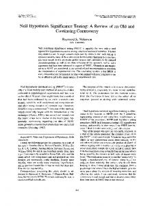
FIG. 1. Temporal distribution of relevant events that occurred during a six-day EEG recording from an epilepsy patient 共lower row: ⫻ seizures, 䊊 subclinical events, 䉭 hyperventilation, and gray vertical bars: discontinuities. Four exemplary seizure time surrogates are displayed in the upper rows. Diamonds denote surrogate seizure onset times established by the constrained randomization procedure described in the text.
that allow one to validate the results of seizure prediction statistics. Given a continuous EEG recording, seizure time surrogates can be constructed by replacing the original seizure times with times randomly chosen from the interictal intervals. Specified properties of the original sequence can be imposed as constraints on the surrogate seizure onset times. Subsequently, any given seizure prediction statistics can be carried out for both the original seizure times and the surrogates. Provided that a preictal state exists and the prediction statistics is able to detect it, the statistics’ performance should be highest for the original seizure times. A similar approach is used in seismology, where null hypothesis tests are regarded as inevitable to evaluate the performance of earthquake prediction algorithms 关11兴. To illustrate this technique, we analyzed the spatiotemporal distribution of a nonlinear measure that was calculated from a quasicontinuous EEG recorded over six days during the presurgical work up 关12兴 of an epilepsy patient independently from the design of our retrospective study. Using implanted electrodes, equipped with a total of 48 separate contacts, the EEG was measured directly at the surface of the cortex and within deeper structures of the brain. The EEG data was sampled at 200 Hz using a 16 bit analog-to-digital converter and filtered within a frequency band of 0.53–100 Hz. Figure 1 shows a scheme of events that took place during the recording time and that have to be taken into account for the generation of surrogate seizure onset times. Twice the patient was briefly 共13 and 54 min兲 disconnected from the EEG acquisition system. A longer discontinuity 共340 min兲 was necessary to carry out a magnetic resonance imaging scan to determine the exact location of the implanted electrodes. All ten seizures occurred spontaneously within the second half of the recording. The latency of the first seizure can be explained by the remaining effect of antiepileptic drugs that were withdrawn after implantation of the electrodes. During the first three days, only three subclinical events took place, i.e., events during which seizurelike activity can be observed in the EEG while the patient does not show any clinical signs of an ongoing seizure. On the third day, the patient was asked to perform a hyperventilation, a seizure provocation technique that may cause alterations of the EEG. For our study, four intervals of 20 min starting at the beginning of both the hyperventilation and the three subclinical events, as well as ten intervals of 1 h starting at the
onset of the seizures were excluded from the analysis. The last step was carried out since the ictal and postictal EEG differs substantially from the EEG recorded during the interictal state. Both these exclusions and the aforementioned discontinuities will be referred to as recording gaps. The remaining length of the analyzed EEG amounted to 101.1 h. In total, 19 seizure time surrogates were generated by replacing original seizure times with times randomly chosen in the interictal intervals 共cf. Fig. 1兲. The following properties of the original seizure times were imposed as constraints on the seizure time surrogates: The total number of seizures (⫽10), the distribution of intervals between consecutive seizures, and the clustering of the seizures in the second half of the recording. The intervals between consecutive seizures and the interval from the first seizure back to an arbitrarily defined starting point T 0 at 12 a.m. on the third day are called D 1 , . . . ,D 10 . For the generation of each of the seizure time surrogates, the following steps were carried out: First, a new starting point was defined as T * 0 ⫽T 0 ⫺(1 h), with being a random number uniformly distributed in 关 0,4兴 . Starting at T * 0 , surrogate seizure onset times * * T 1 , . . . ,T 10 were generated from a random permutation of D 1 , . . . ,D 10 . The sequence was discarded whenever a recording gap was located within the last hour prior to any of *. the T * 1 , . . . ,T 10 As a characterizing measure of the EEG, we used the degree of nonlinear determinism . Following Ref. 关13兴, was defined from a combination of the coarse grained flow average ⌳ 关14兴 and iterative amplitude adjusted surrogates 关15兴. As a direct test for determinism, ⌳ quantifies the alignment of nearby trajectory segments in state space. Here, the use of surrogates is essential to correct an alignment that is caused by autocorrelations rather than by deterministic dynamics. Using a moving-window technique, the EEG was divided into nonoverlapping segments of 20.48 s (N⫽4096 data points兲. For each of these segments, a set of four surrogates was generated. The dynamics were reconstructed using the method of delays 关16兴 with a fixed embedding dimension (m⫽6) and varying time delay . We defined ⬅ 兺 20⫽5 (⌳ EEG ⫺ 具 ⌳ SUR 典 )( ), with ⌳ EEG denoting the value obtained for the EEG segment, and 具 ⌳ SUR 典 denoting the mean value obtained for the surrogates. All parameters were adopted from a previous study in order to avoid any insample overtraining. Only the number of surrogates was reduced from nine to four since the latter value was found to provide a sufficiently reliable estimate of 具 ⌳ SUR 典 . A (t) profile was obtained for each of the 48 EEG channels for segments t⫽1, . . . ,17 764. In order to disregard short-term fluctuations and rather focus on long-term trends of (t), a moving-average filter of 11 consecutive segments was applied. In Ref. 关13兴, we have compared mean values obtained from the interictal EEG recorded from within the epileptic focus and from other brain areas of epilepsy patients. A correct localization of the epileptic focus could be derived from increased values of in all investigated cases. Following the basic concept of Ref. 关2兴, we hypothesized that the preictal
010901-2
RAPID COMMUNICATIONS
PHYSICAL REVIEW E 67, 010901共R兲 共2003兲
TESTING THE NULL HYPOTHESIS OF THE . . .
FIG. 2. Parametrization of an exemplary (t)⫺ 具 典 50 profile. Data from the ictal and postictal state were included for completeness. Gray shaded areas denote interictal peaks (I j ). A preictal peak ( P i ) is shown in black.
state would be reflected in an increase of 共cf. Ref. 关4兴兲, and accordingly designed a simple evaluation for (t) 共Fig. 2兲. First, a reference level was defined by the median 具 典 50 of the distribution of all (t) values for each EEG channel. For every interval B between two crossings of (t) and 具 典 50 , we quantify the area A⫽ 兺 t苸B 关 (t)⫺ 具 典 50兴 . The evaluation was restricted to positive areas, which we will refer to as peaks. Let s denote the number of seizures that were directly preceded by a peak instead of a drop of (t) below the reference level. For those seizures, this peak is termed as preictal and its area is denoted by P i for i⫽1, . . . ,s. All other peaks are termed as interictal and their areas are denoted by I j for j⫽1, . . . ,k, with k being the total number of interictal peaks. The P i were only integrated up to the seizure onset times. In order to compare the distributions of P i and I j , we calculated f ⬅( 具 P i 典 50⫺ 具 I j 典 50 )/( 具 P i 典 50⫹ 具 I j 典 50) from the medians of the two distributions. Finally, we defined F ⬅ 具 f 典 as the average over all channels. By construction, f and F are restricted to 关 ⫺1,1兴 and should tend to zero if the distributions of preictal and interictal peaks match. Figure 3 shows the distribution function of I j along with corresponding values of P i determined for the original seizure onset times for one exemplary EEG channel. Among the s⫽7 preictal peaks, five peaks were found whose area exceeded the median area of the interictal peaks. For this channel, we obtained f ⫽0.94. After averaging the results over all channels, we obtained F⫽0.81 for the original seizure times. At first glance, this value appears quite promising in the sense that it might indicate that the preictal peaks were more pronounced than the interictal peaks, confirming that the preictal state is indeed reflected in an increase of . This interpretation, however, does not necessarily hold: Suppose we selected peaks randomly from a sequence like the one depicted in Fig. 1. If the probability to be selected
FIG. 3. Distribution function prob 兵 area⬍A 其 for interictal peaks I j (line) along with values P 1 , . . . , P 7 (circles) obtained for the original seizure times for one exemplary channel. The two vertical lines indicate the medians 具 I j 典 50 and 具 P i 典 50 , respectively.
FIG. 4. F values for the original seizure times (䊊) and the distribution of 19 seizure time surrogates (⫻).
were the same for all peaks, scores with areas below and above the median of the distribution of areas of all peaks would be equiprobable. If we, in contrast, drew samples from such a sequence by randomly selecting points in time, we would be more likely to draw long peaks than to draw short peaks. Consequently, the area of our samples would tend to exceed the aforementioned median. Taking this into account, a value of F⬎0 would be expected even under the assumption of our null hypothesis. Hence, interpreting the significance of the observed value of F appears quite difficult. One could consider a normalization or correction of F based on the distribution function of I j but this might not be sufficient to eliminate any bias caused by further, unforeseen problems and pitfalls. A more straightforward answer can be obtained from the application of seizure time surrogates. From Fig. 4, it becomes evident that the F value obtained for the original seizure times was within the distribution obtained for the seizure time surrogates. On the level of single EEG channels, i.e., based on f values, the null hypothesis could be rejected for four of the 48 channels. However, if a test with a nominal size of ␣ ⫽0.05 is repeated 48 times, there is a 9% chance to obtain up to four rejections. Hence, we could not reject the null hypothesis of the nonexistence of a preictal state by means of the applied seizure prediction statistics. The fact that the null hypothesis could not be rejected does by no means prove its correctness. Rather, there exist numerous alternative explanations for this result. For several reasons, the applied seizure prediction statistics might simply lack any discriminative power for the hypothesis test: Even though did allow a characterization of the spatial distribution of the interictal epileptic dynamics 关13兴, it may still be incapable to detect any feature of the EEG specific for the preictal state. An explanation for such a finding would be that the interictal epileptic dynamics and the seizuregenerating process are two distinct dynamical phenomena, each imposing different features on the EEG. On the other hand, even if were capable to detect the preictal state, the relevant information could be missed by our rather simple evaluation of (t). Furthermore, our study was based on the EEG recording of only one epilepsy patient. It would be highly speculative to draw any conclusions about the multifaceted disease epilepsy from such a limited sample. It is far beyond the scope of the present study to prove or disprove the existence of a preictal state. Rather, the aim was to propose a simple technique that allows one to validate the performance of seizure prediction statistics. In some cases, e.g.,
010901-3
RAPID COMMUNICATIONS
PHYSICAL REVIEW E 67, 010901共R兲 共2003兲
ANDRZEJAK et al.
if only a collection of very short recordings each containing one seizure is available, a randomization of seizure onset times might not be possible. In these cases, one could randomize the time course of the characterizing measure and keep the original seizure times fixed. For this purpose, the technique of constrained randomization 关9兴 could readily be employed. Further studies are underway which apply seizure time surrogates in combination with different seizure prediction
关1兴 S. Viglione and G. Walsh, Electroencephalogr. Clin. Neurophysiol. 39, 435 共1975兲; Z. Rogowski, I. Gath, and E. Bental, Biol. Cybern. 42, 9 共1981兲; J. Gotman et al., Epilepsia 23, 432 共1982兲; A. Siegel, C. Grady, and A. Mirsky, ibid. 23, 47 共1982兲; L.D. Iasemidis et al., Brain Topogr 2, 187 共1990兲; C. E. Elger and K. Lehnertz, in Epileptic Seizures and Syndromes, edited by P. Wolf 共Libbey and Co, London, 1994兲, pp. 547– 552. 关2兴 K. Lehnertz and C.E. Elger, Phys. Rev. Lett. 80, 5019 共1998兲. 关3兴 J. Martinerie et al., Nat. Med. 4, 1173 共1998兲; I. Osorio, M.G. Frei, and S.B. Wilkinson, Epilepsia 39, 615 共1998兲; F. Mormann et al., Physica D 144, 358 共2000兲; A. Petrosian et al., Neurocomputing 30, 201 共2000兲; K.K. Jerger et al., J. Clin. Neurophysiol. 18, 259 共2001兲; L.D. Iasemidis et al., J. Combinatorial Optimization 5, 9 共2001兲; M. Le Van Quyen et al., Lancet 357, 183 共2001兲; K. Schindler et al., Clin. Neurophysiol. 113, 604 共2002兲; V. Navarro et al., Brain 125, 640 共2002兲; B. Litt et al., Neuron 30, 183 共2001兲. 关4兴 R.G. Andrzejak et al., Epilepsia 41, Suppl. 7 202 共2000兲. 关5兴 H. Kantz and T. Schreiber, Nonlinear Time Series Analysis
statistics and to larger samples of the EEG data to further elucidate the problem of preictal state detection 关17兴. In this context, we expect seizure time surrogates to be a powerful tool to differentiate statistics unsuited for a detection of the preictal state from more promising approaches. We are grateful to Peter Grassberger for carefully reading this manuscript and for valuable discussions. C.E.E., T.K., K.L., F.M., and C.R. acknowledge support from the Deutsche Forschungsgemeinschaft.
关6兴 关7兴 关8兴 关9兴 关10兴
关11兴 关12兴 关13兴 关14兴 关15兴 关16兴
关17兴
010901-4
共Cambridge University Press, Cambridge, U.K., 1997兲. A.R. Osborne and A. Provenzale, Physica D 35, 357 共1989兲. J. Theiler et al., Physica D 58, 77 共1992兲. J. Theiler, Phys. Lett. A 196, 335 共1995兲. T. Schreiber, Phys. Rev. Lett. 80, 2105 共1998兲. P. Rapp et al., Phys. Lett. A 192, 27 共1994兲; J. Timmer, Phys. Rev. E 58, 5153 共1998兲; D. Kugiumtzis, ibid. 60, 2808 共1999兲; P. Rapp et al., Int. J. Bifurcation Chaos Appl. Sci. Eng. 11, 983 共2001兲. Y.Y. Kagan, Geophys. J. Int. 131, 505 共1997兲. Surgical Treatment of the Epilepsies, edited by J. Engel, Jr. 共Raven Press, New York, 1993兲. R.G. Andrzejak et al., Epilepsy Res. 44, 129 共2001兲. D.T. Kaplan and L. Glass, Phys. Rev. Lett. 68, 427 共1992兲. T. Schreiber and A. Schmitz, Phys. Rev. Lett. 77, 635 共1996兲. F. Takens, in Dynamical Systems and Turbulence, edited by D. A. Rand and L.-S. Young 共Springer-Verlag, Berlin, 1980兲, Lecture Notes in Mathematics, Vol. 898, pp. 366 –381. F. Mormann et al., Phys. Rev. E 共to be published兲.