May 13, 2015 - as âshitpostingâ. The vast majority (around 95%) of posts classified by this method are correctly classified, and I have manually removed the ...
Text Classification using Artificial Neural Networks
Fraser Murray May 13th, 2015
Contents
1
2
Introduction
1
1.1
Aim . . . . . . . . . . . . . . . . . . . . . . . . . . . . . . . . . . . . . . . . . . . . . . . . .
1
1.2
Objectives . . . . . . . . . . . . . . . . . . . . . . . . . . . . . . . . . . . . . . . . . . . . .
2
1.3
Requirements . . . . . . . . . . . . . . . . . . . . . . . . . . . . . . . . . . . . . . . . . . .
2
1.4
Deliverables . . . . . . . . . . . . . . . . . . . . . . . . . . . . . . . . . . . . . . . . . . . .
3
1.5
Project scope . . . . . . . . . . . . . . . . . . . . . . . . . . . . . . . . . . . . . . . . . . . .
3
1.6
Report structure . . . . . . . . . . . . . . . . . . . . . . . . . . . . . . . . . . . . . . . . . .
4
Background research
5
2.1
Algorithms . . . . . . . . . . . . . . . . . . . . . . . . . . . . . . . . . . . . . . . . . . . . .
5
2.1.1
Naive Bayes . . . . . . . . . . . . . . . . . . . . . . . . . . . . . . . . . . . . . . . .
5
2.1.2
Perceptron . . . . . . . . . . . . . . . . . . . . . . . . . . . . . . . . . . . . . . . . .
6
2.1.3
Backpropagation . . . . . . . . . . . . . . . . . . . . . . . . . . . . . . . . . . . . .
6
2.1.4
Autoencoder . . . . . . . . . . . . . . . . . . . . . . . . . . . . . . . . . . . . . . .
7
Informal text . . . . . . . . . . . . . . . . . . . . . . . . . . . . . . . . . . . . . . . . . . . .
7
2.2 3
Project background
9
3.1
The problem . . . . . . . . . . . . . . . . . . . . . . . . . . . . . . . . . . . . . . . . . . . .
9
3.2
The solution . . . . . . . . . . . . . . . . . . . . . . . . . . . . . . . . . . . . . . . . . . . .
12
i
4
Project methodology
13
4.1
Schedule . . . . . . . . . . . . . . . . . . . . . . . . . . . . . . . . . . . . . . . . . . . . . .
13
4.2
Technology . . . . . . . . . . . . . . . . . . . . . . . . . . . . . . . . . . . . . . . . . . . . .
14
4.2.1
Naive bayes . . . . . . . . . . . . . . . . . . . . . . . . . . . . . . . . . . . . . . . .
14
4.2.2
Feed-forward neural network . . . . . . . . . . . . . . . . . . . . . . . . . . . . . .
15
4.2.3
Autoencoder . . . . . . . . . . . . . . . . . . . . . . . . . . . . . . . . . . . . . . .
15
4.2.4
Other tools . . . . . . . . . . . . . . . . . . . . . . . . . . . . . . . . . . . . . . . .
15
Conclusion . . . . . . . . . . . . . . . . . . . . . . . . . . . . . . . . . . . . . . . . . . . . .
16
4.3 5
6
Design & implementation
18
5.1
Naive Bayes classifier . . . . . . . . . . . . . . . . . . . . . . . . . . . . . . . . . . . . . . .
18
5.2
Perceptron . . . . . . . . . . . . . . . . . . . . . . . . . . . . . . . . . . . . . . . . . . . . .
19
5.3
Feed-forward neural network . . . . . . . . . . . . . . . . . . . . . . . . . . . . . . . . . .
19
5.4
Autoencoder . . . . . . . . . . . . . . . . . . . . . . . . . . . . . . . . . . . . . . . . . . . .
20
5.5
Other tools . . . . . . . . . . . . . . . . . . . . . . . . . . . . . . . . . . . . . . . . . . . . .
20
5.5.1
20
Automatic evaluation script . . . . . . . . . . . . . . . . . . . . . . . . . . . . . . .
Evaluation methodology
21
6.1
Measuring relevant performance . . . . . . . . . . . . . . . . . . . . . . . . . . . . . . . . .
21
6.2
Dataset . . . . . . . . . . . . . . . . . . . . . . . . . . . . . . . . . . . . . . . . . . . . . . .
23
6.3
Algorithms to evaluate . . . . . . . . . . . . . . . . . . . . . . . . . . . . . . . . . . . . . .
23
6.3.1
Naive Bayes classifier . . . . . . . . . . . . . . . . . . . . . . . . . . . . . . . . . .
23
6.3.2
Perceptron and backpropagation . . . . . . . . . . . . . . . . . . . . . . . . . . . .
24
6.3.3
Autoencoder . . . . . . . . . . . . . . . . . . . . . . . . . . . . . . . . . . . . . . .
24
Environment . . . . . . . . . . . . . . . . . . . . . . . . . . . . . . . . . . . . . . . . . . . .
24
6.4.1
24
6.4
Machine specs . . . . . . . . . . . . . . . . . . . . . . . . . . . . . . . . . . . . . .
ii
7
8
6.5
Hypothesis . . . . . . . . . . . . . . . . . . . . . . . . . . . . . . . . . . . . . . . . . . . . .
25
6.6
Conclusion . . . . . . . . . . . . . . . . . . . . . . . . . . . . . . . . . . . . . . . . . . . . .
25
Performance evaluation
26
7.1
Precision . . . . . . . . . . . . . . . . . . . . . . . . . . . . . . . . . . . . . . . . . . . . . .
26
7.1.1
Naive bayes implementations . . . . . . . . . . . . . . . . . . . . . . . . . . . . . .
26
7.1.2
Neural networks . . . . . . . . . . . . . . . . . . . . . . . . . . . . . . . . . . . . .
27
7.1.3
Autoencoder . . . . . . . . . . . . . . . . . . . . . . . . . . . . . . . . . . . . . . .
27
7.2
Classification time . . . . . . . . . . . . . . . . . . . . . . . . . . . . . . . . . . . . . . . . .
29
7.3
Conclusion . . . . . . . . . . . . . . . . . . . . . . . . . . . . . . . . . . . . . . . . . . . . .
30
Conclusion
31
8.1
Limitations . . . . . . . . . . . . . . . . . . . . . . . . . . . . . . . . . . . . . . . . . . . . .
31
8.2
Potential improvements . . . . . . . . . . . . . . . . . . . . . . . . . . . . . . . . . . . . . .
31
8.3
Methodology evaluation . . . . . . . . . . . . . . . . . . . . . . . . . . . . . . . . . . . . .
32
8.4
Objectives . . . . . . . . . . . . . . . . . . . . . . . . . . . . . . . . . . . . . . . . . . . . .
32
8.5
Requirements . . . . . . . . . . . . . . . . . . . . . . . . . . . . . . . . . . . . . . . . . . .
33
8.6
Deliverables . . . . . . . . . . . . . . . . . . . . . . . . . . . . . . . . . . . . . . . . . . . .
33
8.7
Overall conclusion . . . . . . . . . . . . . . . . . . . . . . . . . . . . . . . . . . . . . . . . .
33
A Materials used
35
A.1 Libraries . . . . . . . . . . . . . . . . . . . . . . . . . . . . . . . . . . . . . . . . . . . . . .
35
A.1.1
Diagrams . . . . . . . . . . . . . . . . . . . . . . . . . . . . . . . . . . . . . . . . .
35
A.1.2
Chart . . . . . . . . . . . . . . . . . . . . . . . . . . . . . . . . . . . . . . . . . . . .
35
A.1.3
Cassava . . . . . . . . . . . . . . . . . . . . . . . . . . . . . . . . . . . . . . . . . .
35
A.1.4
HNN . . . . . . . . . . . . . . . . . . . . . . . . . . . . . . . . . . . . . . . . . . . .
36
A.1.5
Reddit . . . . . . . . . . . . . . . . . . . . . . . . . . . . . . . . . . . . . . . . . . .
36
iii
B Ethical issues
37
C Code listings
38
C.1 Package data-counter . . . . . . . . . . . . . . . . . . . . . . . . . . . . . . . . . . . . . C.1.1
38
Data.Counter . . . . . . . . . . . . . . . . . . . . . . . . . . . . . . . . . . . . . .
38
C.2 Package naive-bayes . . . . . . . . . . . . . . . . . . . . . . . . . . . . . . . . . . . . . .
40
C.2.1
Data.Classifier . . . . . . . . . . . . . . . . . . . . . . . . . . . . . . . . . . . .
40
C.2.2
Data.Classifier.NaiveBayes . . . . . . . . . . . . . . . . . . . . . . . . . . .
41
C.3 Package project-utilities . . . . . . . . . . . . . . . . . . . . . . . . . . . . . . . . .
42
C.3.1
pull-comments . . . . . . . . . . . . . . . . . . . . . . . . . . . . . . . . . . . . .
42
C.3.2
comment-to-arff . . . . . . . . . . . . . . . . . . . . . . . . . . . . . . . . . . . .
46
C.3.3
produce-results . . . . . . . . . . . . . . . . . . . . . . . . . . . . . . . . . . . .
47
C.3.4
parse-output . . . . . . . . . . . . . . . . . . . . . . . . . . . . . . . . . . . . . .
53
C.3.5
chart-generator . . . . . . . . . . . . . . . . . . . . . . . . . . . . . . . . . . . .
56
D Raw evaluation results
63
D.1 Laptop results . . . . . . . . . . . . . . . . . . . . . . . . . . . . . . . . . . . . . . . . . . .
64
D.2 Desktop results . . . . . . . . . . . . . . . . . . . . . . . . . . . . . . . . . . . . . . . . . .
66
Bibliography
69
iv
Chapter 1
Introduction For my project, I intend to develop a neural network-based algorithm to classify internet gaming forum posts into two categories based on their content—those whose authors are new to the game and may need advice, and unrelated posts whose content may cover anything else related to the game. The game itself can be intimidating for newer players, and many of them ask others for help in getting started. Since the majority of new players simply don’t know where to start, the best advice is often just giving them a list of guides and other information they can learn from. As there can be lots of similar posts from new players, it can become tedious responding to them with almost identical replies. Ideally there would be a bot which watches for new posts and deals with posts appropriately—by responding to posts that the algorithm identifies, while ignoring other posts. The objective of this project will be to develop this bot, with more of a focus on the algorithms involved in creating the classifier and less about the surrounding code used for the bot’s automation. However, the ultimate use for the classifier will be integral when considering the evaluation of the classifiers, and the Project Background section of this report will go into greater detail on the classifier’s intended use in order to provide more context.
1.1
Aim
The ultimate aim of the project is to develop a classifier which can accurately detect which of the posts submitted by users are written by new players asking for help. The ideal outcome of the project will be to have a working fully-automated bot powered by an algorithm which can correctly identify the type of 1
the majority of posts.
1.2
Objectives
My objectives for the project are: • Implement a baseline naive Bayes classifier • Evaluate the naive Bayes classifier’s performance on my data set • Compare my own implementation’s evaluation with an evaluation using Weka’s reference implementation • Implement a classifier using a feed-forward neural network (using a backpropagation algorithm), and evaluate it using my test data • Implement an autoencoder, and evaluate it using my test data • Implement a deep belief network classifier, and evaluate it using my test data At minimum, I expect to be able to create a classifier with the feed-forward network, as well as one or both of the autoencoder and deep belief network, time permitting.
1.3
Requirements
My minimum requirements for my project are closely linked to the objectives. My requirements are: • Implement a naive Bayes classifier of my own, evaluate it and compare it to Weka’s implementation • Implement a feed-forward neural network-based classifier, and compare it to Weka’s implementation • One of the following, depending on available time: – Implement an autoencoder, use it to create a classifier, and then evaluate it – Implement a deep belief network, use it to create a classifier, and then evaluate it
• Compare the different algorithms to determine which will be most suitable for solving the problem 2
1.4
Deliverables
The deliverables for the project will consist of a few different components, which are outlined below: • The project report – This document will be the main deliverable for the project, detailing the process I used for the
entire project, as well as my own evaluation of the results found • Code written – The code portion of the deliverables for the project will be comprised of a series of Haskell
packages, as outlined below: * The data-counter package * The naive-bayes package * The project-utilities package, consisting of multiple scripts to “glue” the code together · A script for conversion of data from the raw post format into the formats used by the algorithms · A command-line tool for automatically testing data en masse based on parameters given · A program for parsing results from tool for automatic testing · A chart generator to create images from the CSV results output • Table of results with the raw results from the project-utilities tool
1.5
Project scope
The project will not cover any of the code for the operation of the bot—the raw content of the posts will be passed to the algorithm, which will then extract the features from the post’s text body and convert them into the different formats required for each algorithm’s input. The library code for interfacing between the Reddit website and the automated bot will not be part of the project’s scope, but the classifier’s intended use will be taken into account when considering the evaluation criteria.
3
1.6
Report structure
Chapter 2 explores similar work that has already been done in the field, and explains how I will learn from and expand on the results. Chapter 3 expands on the project definition in this chapter, explaining how the classifier will be used, as well as some of the reasons for why certain evaluation criteria were chosen. Chapter 4 goes into detail on the time scale set aside for the project, as well as the technology used to produce the deliverables. Chapter 5 describes which algorithms I will be evaluating, as well as the methods I will be using to convert the raw post data into an appropriate format for the algorithms chosen. It will also cover decisions made when implementing my own versions of some of the algorithms used. Chapter 6 shows my methodology for evaluations the algorithms involved, and expands on how I compared the different techniques and their performance on the data set. Chapter 7 shows the results I found as a result of my evaluation, exploring the results and how they can apply to the dataset and the overall problem. Chapter 8, the conclusion, will outline my final thoughts on the project, as well as any potential avenues to explore in the future.
4
Chapter 2
Background research In this chapter, I outline the existing research in this area.
2.1
Algorithms
2.1.1 Naive Bayes The core of the naive Bayes classification technique is the application of Bayes’ theorem,¹ a theorem that states how current probabilities are related to previous possibilities (Laplace, 1812). The so-called “naivety” of the classifier comes from its assumption that all of the features used in classification are independent from eachother. While this assumption is rarely true, and may seem unreasonable, the classifier is—given effective pre-processing of the data—comparable to newer and more complicated machine learning techniques (Rennie et al., 2003). By assuming different distributions in the input features and applying Bayes’ theorem, one can estimate the chance that a given instance belongs to a certain class. Typically text categorisation will use a multinomial or multivariate model (Kibriya et al., 2005), with the multinomial event model usually performing more favorably; this is the model I will be using for my baseline classifier. Due to their simple implementation and solid performance, naive Bayes classifiers are often used as baselines with which to compare newer classifiers. ¹Bayes’ theorem states that P (A|B) =
P (B|A)P (A) . P (B)
5
2.1.2 Perceptron Invented in 1957 by Frank Rosenblatt, the perceptron algorithm is a technique for the supervised learning of linearly separable classifiers using artificial neurons. While the algorithm is by itself only capable of properly learning linearly separable classifiers, with appropriate feature selection, it can yield impressive results (Ng et al., 1997). The basic algorithm works by modeling an artificial neuron which activates in response to its inputs, yielding a binary (true or false) result.
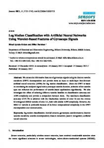
2.1.3 Backpropagation By combining multiple neuron layers together and adapting the perceptron algorithm (such that the derivation of the final error can be traced or “propagated” backwards to previous layers), one can create a neural network trained to replicate classifiers which are not linearly separable. By utilizing multiple layers, the network is able to adjust itself in order to extract non-linear features. In Text Categorization by Backpropagation Network (Ramasundaram and Victor, 2010), this process is used in conjunction with techniques like stemming, stop word removal, and various forms of dimensionality reduction in order to train a neural network to classify text.
Output layer Hidden layer 2
Hidden layer 1
Input layer
Figure 2.1: Architecture of a feed-forward neural network. With the backpropagation algorithm, a network like this can be trained to approximate a given function.
6
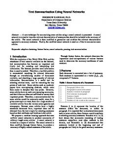
2.1.4 Autoencoder Autoencoders are artificial neural networks whose purpose is to perform dimensionality reduction by creating a compressed version of any input data. The simplest form of autoencoder is simply a feed-forward neural network trained via backpropagation to learn the identity function—while this may seem counterproductive, by restricting the size of the single hidden layer the network learns which of the features are more important to the overall input data (Vincent et al., 2010) (Bengio, 2009).
Hidden layer
Input layer
Output layer
Figure 2.2: Architecture of a autoencoder built from a feed-forward neural network. This autoencoder will compress an layer with five nodes into a layer with two nodes, creating an encoder (to compress a layer down to two nodes) and a matching decoder (to convert the two-node layer back into an approximation of the original five-node layer).
2.2
Informal text
While there has been some research done into analysing informal text (Thelwall et al., 2010), with an emphasis on learning features of text which does not necessarily follow strict and correct grammar, I will not be focusing on this aspect of my dataset, and won’t be applying any special techniques to my evaluation to make use of this heuristic.
7
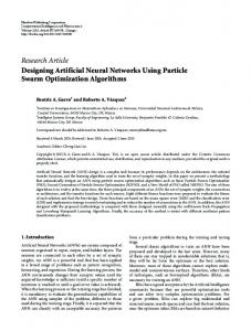
Encoder
Decoder
Figure 2.3: A paired encoder and decoder created from the neural network shown in Figure 2.2. The left hand side (the encoder) represents the weight vector which transforms the input feature vector into its compressed form, and the right hand side is the decoder whose intended purpose is to decompress the smaller feature vector back into its original form.
8
Chapter 3
Project background The main problem to be solved with this project is the issue is automating responses to new player posts on an internet forum. This will improve the forum experience for both the users giving and receiving advice: by reducing the number of repetitive submissions, and by ensuring that new players get the advice that they need.
3.1
The problem
Figure 3.1: Figure showing the Reddit front page, displaying a list of submissions. Reddit is a website which allows users to post content, such as links or text posts. Links allow users to submit a web URL to the site, whereas text posts allow them to add a block of text to their submission— 9
this project will not involve any use of link posts, and will concentrate solely on the text or “self” posts (mainly their body text content). Other Reddit users can then reply to the posts with comments, which in turn can be responded to individually, creating a tree of nested comments. While the techniques and algorithms used in this project could be extended to work with comments, the project will only focus on posts. Both posts and comments can be voted on by other Reddit users—casting a positive vote (or “upvoting”) content raises it higher in the listing, while casting a negative vote (or “downvoting”) lowers its ranking. The concept of voting on submissions and comments is core to the site, as the score of the content is directly tied to its perceived value in the community. Users can also create smaller focused communities dedicated to certain topics, for example video games, politics, or news. Users who create a so-called “subreddit” are given moderation power over the communities they create, allowing them a certain amount of control over their section of the main site. These powers include the ability to prevent users from posting on their subreddit, to remove individual posts, or to add other moderators. Other users can then “subscribe” to any subreddits that they’re interested in, allowing posts from that particular subreddit to appear in their posts feed. Unfortunately, as a subreddit grows in subscriber count, the quality of its content often drops considerably, due to a few factors. While some of these factors are entirely out of the moderators’ control, such as the gradual decline of in-depth content, (due to the increased accessibility of low-effort posts and comments which can be more easily read and voted upon) some of the problems can be dealt with by enforcing strict moderation or by encouraging users to post high-quality content. Automating the moderation of subreddits can often be an effective way to increase the overall quality of content without moderators committing significant effort to enforcing rules.
Figure 3.2: Figure showing a screenshot of an in-progress game of Dota 2. Dota 2 (“Dota 2 blog,” 2015) is a video game developed by Valve Corporation notorious for its steep learning 10
curve and hostile community. Because of this, new players can often be quickly put off, and typically either stop playing or turn to the internet for help. One of the most common types of repeated submission in the Dota 2 subreddit is the “I’m new to the game and don’t know what to do” post, and while the community has a prominent link to some basic guides for new players, most newcomers either need more specific advice, or don’t see the “guides” link. However, more experienced Dota 2 players on Reddit are often irritated by newer users asking for assistance (as a result of the frequency of new player posts) which can sometimes alienate new players.
Figure 3.3: An example of a new player post asking for help with learning the game. Figure 3.3 shows an example of a new player submitting a post asking for help, and while the grammar in this particular example is fairly formal, the vast majority of “I’m new” posts employ very informal English, with shortened words such as “you” substituted with “u”, emoticons like “:)” and “( ͡° ͜ʖ ͡°)”, or a total lack of capitalisation.
Figure 3.4: An example of a new player post containing emoticons and incorrect capitalisation, and therefore does not require a response. 11
3.2
The solution
At the moment, the standard response to these new player posts is linking them to the subreddit’s guides, but this process could be simplified by automating the posting of guides for the new players. By taking into account the textual content of the posts, it should be possible to automatically detect which posts have been created by new players asking for help, and which posts are regular content.
Figure 3.5: An example of a submission that isn’t by a new player. By utilising machine learning techniques, my intention is to create an automated bot that can watch for new posts, correctly separate them into two different classes (new player and otherwise), and respond instantly to new players with useful guides and information to help them get started playing the game.
12
Chapter 4
Project methodology 4.1
Schedule
The schedule as follows was devised on the week beginning February 9th 2015: • February 20th – Have naive Bayes classifier implemented and evaluated
• March 20th – Have feed-forward neural network classifier implemented and evaluated
• April 17th – Have autoencoder-based classifier implemented and evaluated
• Time permitting – Implement and evaluate a deep belief network classifier
Unfortunately, due to a variety of factors, mainly the exploratory nature of the project (as well as implementation obstacles and illness), the schedule was delayed by almost a week. This delay is not reflected in the above schedule, as unforeseen problems were anticipated when the project work began.
13
Week no.
0
1
2
3
4
5
6
7
8
9
10 11 12 13
Naive Bayes implementation / evaluation Backpropagation implementation / evaluation Autoencoder implementation / evaluation Evaluation analysis / report writing
Figure 4.1: A Gantt chart to show the intended project schedule
4.2
Technology
When deciding on which technologies to incorporate into my project, I took into account a number of factors, including my familiarity with each tool as well as the fitness of the tool for the purpose.
4.2.1 Naive bayes For the reference implementation of the Naive-Bayes algorithm, I decided to use the powerful Weka (Hall et al., 2009) software suite, a Java program with a number of in-built classifiers which includes a flexible Naive-Bayes implementation. Weka also features a number of filters which can be applied to data before a classifier is built, including a basic StringToWordVector filter which converts a block of unstructured text into its separate words in order to allow for feature extraction. As I have previously used the Weka software in my second-year Artificial Intelligence module as well as my third-year Text Analytics module, I have become quite familiar with Weka’s features for text analysis and feel confident using it for my reference implementation. Having only studied the theory behind the Naive-Bayes algorithm, I decided to implement my own version rather than use another off-the-shelf implementation. I wanted to further my knowledge by implementing it from scratch by myself, and as one of the most simple and well-documented machine learning algorithms, I expected to be able to produce a working implementation in less than a week. I decided to build my own implementation of Naive-Bayes using the Haskell programming language (Jones, 2003). While I could have used one of the myriad other programming languages suited to this task (including Python (“About python,” 2015), R (Tippman, 2015), and Julia (“The julia language,” 2015)), I decided to use Haskell due to my familiarity with it as well as its strong safety guarantees. Despite there being 14
relatively little chance of running into any security-related problems with the task at hand, its strong static type system allows mathematical code (e.g. an algorithm implementation) to be written without needing to worry about problems other languages may encounter, such as null pointer exceptions and out of bounds errors (Hudak and Jones, 1994). Even though the existing code for the rest of the bot is written in Haskell, it would be relatively simple to produce the core of the algorithm in another language, sending the data into the other program and receiving the results back—however, for the reasons outlined above I have decided to use Haskell.
4.2.2 Feed-forward neural network I again decided to use Weka for the feed-forward network, as my use of the tool for the Naive-Bayes reference implementation means that it will be near-trivial to use the same data with a different algorithm. Simply by selecting the MultilayerPerceptron classifier in Weka, I was able to easily get Weka to generate a feed-forward neural network binary classifier for the problem. For the second implementation of the backpropagation algorithm, I decided to use hnn, the Haskell neural network library (Mestanogullari and Johnson, 2014). The library includes a flexible interface for creating classifiers with backpropagation, which meant it was simple for me to test multiple neural network architectures by varying different parameters.
4.2.3 Autoencoder For my implementation of the autoencoder, I decided to again use the hnn library. By using backpropagation to train a feed-forward neural network with a single hidden layer of a fixed number of nodes, it’s possible to create a compressed version of each input. A new feed-forward network can then be trained to classify the compressed version of the input.
4.2.4 Other tools As well as considering the technologies to use for the core algorithms my project will use, I also needed to decide which programming language I would use to create the scripts to allow the algorithms and data to interface, as well as programs for handling the classifier evaluation itself. The five components of this “glue” code are outlined below:
15
• Reddit post retrieval – This script will retrieve all the relevant (i.e. new player) posts using the Reddit API to use as
the training and test dataset, as well as a selection of non-relevant posts. • Post to ARFF converter – This script will convert the Reddit posts from the custom format to the standard Attribute-
Relation File Format (ARFF) used by Weka. • Evaluate classifiers’ performance – This script will apply each classifier to the dataset, providing an output file with each generated
classifier alongside its performance evaluation. • Classifier performance log parser – This script will parse the output from the classifier performance log and generate a comma-
separated value (CSV) file with the recorded metrics from all the evaluations. • Chart generator – This script will process the CSV file and generate relevant charts for this document.
The two main contenders for the programming language I would use to create these tools were Python and Haskell. Both languages have mature, stable libraries which would allow me to complete all of these tasks easily, but in the end I decided to use Haskell, mainly due to my previous decision to use Haskell for all the rest of the code—converting the dataset back and forth between the two languages for each task would likely have proved too much work for very little gain.
4.3
Conclusion
In conclusion, the main parts of my project will all be using Haskell libraries, either ones that I have already written mysef, or are already existing. The complement will be made up by Weka for the existing implementations of two of the algorithms. Unfortunately due to time constraints, I was unable to work on a deep belief network version of the classifier, for which I would have used the Theano library due to its suitability for deep learning tasks (Bergstra et al., 2010). I could have used it for my own implementations of the algorithms as well, but my 16
lack of familiarity with the library meant I was apprehensive toward trying to learn it from scratch while at the same time implementing an algorithm with which I don’t have much experience.
17
Chapter 5
Design & implementation In this section, I will explore my implementation and uses of the different algorithms, as well as the reasons behind the decisions I made as I wrote my code.
5.1
Naive Bayes classifier
The naive Bayes family of classifiers all base their operations by assuming that all of the input features are completely independent. While this assumption is rarely true, the classifiers are often impressively accurate (Zhang, 2004), and it’s for this reason that naive Bayes classifiers are commonly used as a baseline classifier when comparing other algorithms. Since my features are word counts, I decided to implement the multinomial variant of the classifier, which takes into account the number of times each feature occurs in the input. I implemented the naive Bayes classifier using Haskell’s Map data type, which is implemented using sizebalanced binary trees, as described in Efficient Sets: A Balancing Act (Adams, 1992). By counting the frequency of words in each class, the number of instances in each class, and the number of words in the entire corpus, I built a structure which is able to efficiently learn an instance with just four Map intersections. My implementation is also able to perform online training of data points—that is, the entire training set does not need to be available when training begins. When evaluating the Bayes classifier, I take advantage of the fact that the classifier is a mathematical group; instead of having to re-train the entire classifier in order to test the classifier on a single data point
18
using n-minus-one (also known as leave-one-out) cross-validation, I can simply erase that element from the existing classifier by multiplying the built classifier by the inverse of the instance to be removed.
5.2
Perceptron
As a perceptron is simply a feed-forward neural network with no hidden layers trained with backpropagation (which is the same as the perceptron algorithm when applied to a network with no hidden layers), this “algorithm” is only in this section for completeness’ sake. By telling HNN to simply build a network with |vocabulary| input nodes and one output node, the library creates a network which is functionally identical to a basic perceptron, representing the weights as a single matrix with dimensions (|vocabulary| + 1) × 1. By modifying the weights depending on the final error, the perceptron gradually
learns a more and more accurate representation of the classifier. As with the other neural network implementations I tested, a learning rate of 0.8 was used for all the evaluations.
5.3
Feed-forward neural network
Internally, HNN represents the weights between nodes in a neural network as a stack of matrices. For example, a neural network with a 9-node input layer, a single 5-node hidden layer and a 2 node hidden layer is represented by a pair of matrices, the first with dimensions 10×5, and the second with dimensions 6 × 2. The backpropagation algorithm is applied to these matrices repeately in order to train the network.
By converting each instance of my textual data to a vector of ones and zeros (one representing “this word is present in the instance” and zero representing “this word is not present in the instance”), I can multiply the input vector by each of the matrices in the stack in turn to return a single-element vector representing the classification of the instance. By calculating the error in the output and propagating it backwards through the layers (hence the name) All of the neural network implementations were tested with a learning rate of 0.8.
19
5.4
Autoencoder
The implementation of the autoencoder was relatively simple once I managed to get the feed-forward neural network functioning with the HNN library. By creating a neural network in HNN with x input and output nodes, and a single hidden layer with y nodes, I can split the two halves of the network into two sets of weights—one for compressing (or encoding) the set of input nodes, and another for decompressing (or decoding) the compressed version back to an approximate recreation of its output nodes. Applying this encoder to my input vectors yields a compressed version of my input, which I can then feed into a new perceptron or feed-forward neural network in order to generate a (hopefully more performant) classifier.
5.5
Other tools
As well as getting the algorithms to work, I also needed a few scripts to quickly and automatically obtain the results I needed, so that I could easily launch the scripts on each of the machines on which I evaluated the algorithms.
5.5.1 Automatic evaluation script My initial prototype of this script only included the ability to create a single neural network with a specified architecture, trained a certain number of times, and to evaluate it, printing the evaluation results to the console. I would then have to manually copy and paste the results into a spreadsheet in order to check the results. This was slow, error-prone and tedious, so over time I added many different features to the script, including: • The ability to record the time it took to create each classifier, and how long it took to classify the entire test dataset • A simple way for me to automatically test multiple architectures, while recording their metrics after many different training epochs—for example, the script tracks the performance after 10, 20, 30, etc. epochs, all the way up to 9000 • The ability to take the evaluation logs and convert them to the CSV file format, allowing for me to directly import the logs into a spreadsheet program and browse them
20
Chapter 6
Evaluation methodology Since the core of this project is to compare the performance between different algorithms, the criteria used to determine which of the algorithms perform best are of critical importance. This section outlines the method for evaluating the different algorithms.
6.1
Measuring relevant performance
When considering which of the performance characteristics to use for my evaluation, my main concern was for the intended use of the classifier. For each algorithm evaluation, I decided to record five primary values relevant to their performance: • Time taken to generate the classifier – I measured the total duration taken to generate the classifier from the training dataset.
• Time taken to classify instances – I measured the total duration required to classify the entire test dataset.
• Precision – Defined as
|relevant∩retrieved| , |retrieved|
precision denotes the number of documents which were classi-
fied positively relative to the number of correctly-classified positive documents. • Recall
21
– Defined as
|relevant∩retrieved| , |relevant|
recall is the number of documents which were classified pos-
itively relative to the number of documents which would be returned if the classifier was perfect. • Total percentage correct – While I am recording the total percentage of documents that the classifier correctly classifies,
this measurement is often less useful than precision and recall since it offers less context about how well the classifier performed. The two main attributes of each classifier that I will be taking into account will be precision and classification time. Precision is very important in the context of the bot, as a false positive means that a potentially offensive comment will be posted—responding to an unrelated post with a message saying “you look like you are new to the game” could quite easily be interpreted as insulting, even if the recipient is aware that the message was sent by an automated bot. The time taken to classify each post is also fairly important for the bot, since a slow classification time will result in unread posts queueing up. If the time taken to classify is too long (i.e. longer than the average time between two submitted posts), the queue of un-classified posts will build up indefinitely, rendering the bot essentially useless—however, it would be impossible to give a concrete upper bound on the available time for the classification: the mean time between posts can vary massively over time, and is very likely to only increase over time. Another consideration here is that the finished bot will be running on a virtual private server with much less processing power than either of the two machines on which I will be evaluating the algorithms. While the time taken to generate the classifier will be considered, this metric is much less pertinent to the task, as the dataset can be pre-processed on another machine beforehand and the classifier stored on disk. This means that the classifier can be generated once and kept to use in the classification later. However, classifiers which take a significant period of time to create pose a problem with regards to evaluation: this project is limited by time constraints and I am unable to test multiple classifiers if their creation takes a long time. I will be practically ignoring the “total percentage correct” metric as paying attention to precision and recall is almost universally better and offers me much more context as to whether the algorithms’ evaluations are useful in the context of the whole project. However, the recall statistic is less important to me, as false negatives are easily remediated; similar to how the dataset was created (as outlined below), users can manually flag a submission as relevant for the bot to automatically respond to it. If a post is missed by the classifier, it’s trivial for someone else to manually classify it, meaning the cost of a false 22
negative is very low. A high total correct value can also be misleading as a result of the imbalanced class counts—the number of negatively-classified posts is much greater than the number of positively-classified posts, meaning that simply ignoring the input entirely and classifying every post as negative yields a total of 81% correct classifications.
6.2
Dataset
Due to the difficulties in creating a synthetic dataset for this problem, I decided to use a real dataset for the evaluation of the classifiers. Over the past year, a simplistic version of the automated bot has been active on the Dota 2 subreddit, which allows users to flag a post by mentioning its username in a comment reply. By checking every submitted comment reply for its own username, the bot is able to mark a post as belonging to the positive class. While this semi-automated approach has worked in the vast majority of cases, some users have used the ability to post by proxy to insult others in a comedic manner, as a form of the act known on Reddit as “shitposting”. The vast majority (around 95%) of posts classified by this method are correctly classified, and I have manually removed the positive classification for the others by scouring the dataset by hand. By using Reddit’s API in conjunction with my own Haskell Reddit library, I was able to retrieve the entire set of positively-classified submissions, as well as a randomised selection of unrelated (negativelyclassified) posts, and these two groups of posts are combined to form my dataset.
6.3
Algorithms to evaluate
While my planning for the specific algorithms for evaluation is shown below, due to the exploratory nature of the project, it’s difficult to predict which of them will yield the most promising results and should be explored further.
6.3.1 Naive Bayes classifier As a baseline, I will use my implementation of the naive Bayes classifier to set a minimum evaluation standard which I would hope all other algorithms will meet. I will apply the Weka naive Bayes implementation to the same dataset to see if the results differ significantly.
23
6.3.2 Perceptron and backpropagation For the perceptron evaluation, I will simply train a perceptron to classify the dataset. There are very few parameters to tweak with a perceptron (apart from learning rate, which I will be keeping constant throughout all of my evaluations), so the main result will be from training the simple perceptron many times. Due to the time constraints of the project, I will be focusing my efforts on evaluating neural networks with one or two hidden layers, as these will be the quickest to train while hopefully still yielding significant results. I will experiment more with 3-layer networks (i.e. one hidden layer) due to 4-layers networks’ increased likelihood of getting stuck in a local minima (De Villiers and Barnard, 1993).
6.3.3 Autoencoder In order to evaluate the autoencoder technique, I will create a feed-forward neural network with a small hidden layer and identical input and output patterns. Once the network has been sufficiently trained, I will separate the two weight matrices into an encoder and decoder, and use the encoder to compress my entire test dataset. By training another feed-forward network using this compressed dataset, I will hopefully be able to more train a network using the compressed feature set from the encoder.
6.4
Environment
In order to assess the performance of the different algorithms, I will run my tests on two machines: a laptop and a desktop. The specs of the two computers are listed below—since the algorithms are all primarily CPU-bound, the processors of the machines will likely be the most important and relevant statistic.
6.4.1 Machine specs • Laptop – Mid-2013 MacBook Air – Intel Core i3 processor at 1.3GHz – 4GB memory – Tests performed on Mac OS X
24
• Desktop – Custom-built desktop – Intel Core i5 processor at 3.2GHz – 8GB memory – Tests performed on a Linux virtual machine running on a Windows hosts
6.5
Hypothesis
I expect that the naive Bayes classifier will be very fast—the algorithm itself is not particularly processorbound and is relatively simple. Due to its reputation as a useful baseline, I expect that it will also perform fairly well, but not as well as the feed-forward neural network classifier. I would anticipate that the autoencoder will turn out to be slower and less effective than either of the other two algorithms due to it needing a long time to generate the encoder-decoder pair and the likelihood of taking a significant amount more work to generate a encoder that’s actually useful.
6.6
Conclusion
Each of the algorithms will be tested on the dataset, which will provide the metrics required to make a decision regarding the optimal method of classification. While the combination of precision and classification time will be my primary factors to consider, there is no simple way for me to categorically decide which algorithm is strictly better, and I will have to use the evaluation results to decide which algorithm to implement in the finished bot.
25
Chapter 7
Performance evaluation This section presents the evaluation of each of the algorithms and compares their results in order to determine which of the classifiers is best suited for the purpose—that is, for classifying post submissions as the core algorithm of the automated bot. The table containing all of the evaluation results can be located in Appendix C.
7.1
Precision
7.1.1 Naive bayes implementations Table 7.1: Comparison of the Weka naive Bayes implementation and my own naive Bayes implementation
Weka
Mine
True positive
546
524
True negative
2474
2399
False positive
180
255
False negative
73
95
75.2%
67.3%
Precision
26
While my own implementation of the multinomial naive Bayes classifier performs slightly worse than the Weka version, the two are similar enough that I feel confident that I have implemented the algorithm correctly. The difference in their evaluations can likely be attributed to the tokenisation—Weka’s StringToWordVector is purpose-built for extracting words from a block of text, whereas my process
function simply removes hyphens, splits on periods and spaces, and then removes non-alphanumeric characters. This basic approach works well, but falls short of the more complex algorithm used by Weka.
7.1.2 Neural networks On both machines, the results showed that the feed-forward neural network with one 10-node hidden layer performed the best of all the network evaulations with regard to precision, but it also found that the backpropagation algorithm was prone to overfitting, and the precision actually decreased again after a certain number of training epochs. For example, on the laptop, the best neural network evaluation was the 10-node single hidden layer network after 3000 epochs, achieving a precision value of 75.1%, but it deteriorated as it was trained more, with a precision of 74.3% after 6000 epochs, and with a miserable 21.9% precision after 9000 epochs. This was likely due to eventual overfitting of the training data, which meant that the classifier would perform worse on the other test dataset. I found a similar but less pronounced result with the desktop, where the same single layer 10-node network performed best at 8000 epochs (with 70.0% precision), but dropped to 68.0% after 9000 epochs. The Weka implementation of the feed-forward neural network classifier performed abominably, taking a full week to generate a 504-layer neural network which barely achieved a higher precision than the HNN perceptron trained just 10 times. As this result seems uncharacteristically bad for Weka, the problem is more likely to be me operating the program incorrectly rather than Weka performing badly. I would have liked to try and get the implementation to work better, but due to time constraints I couldn’t justify spending entire weeks experimenting on a reference implementation of a classifier.
7.1.3 Autoencoder The autoencoder implementation with a compressed size of 10 (i.e. 10 hidden nodes in the creation network) performed incredibly badly, and was utterly useless after being trained with a perceptron, classifying every single instance as a positive. While this meant its recall was incredibly impressive (100%), it has no use as it’s worse precision-wise than totally random guesses would be. I would have liked to test the
27
Figure 7.1: Chart showing the relationship between precision and recall as the perceptron over epochs as the perceptron is trained on the desktop. While the recall value decreasing as the network is trained may seem like a problem, it is simply a side effect of the network becoming more stringent in which instances it classifies positively.
Figure 7.2: Chart showing the relationship between precision and the number of training epochs for each of the architectures trained on the desktop. Due to time constraints, different architectures were trained for different maximum epochs. The plateaus visible on the perceptron ([]) precision are likely a result of the algorithm becoming stuck in a local minimum—the sharp increases in precision are a result of the evaluation method: rather than use the same perceptron from 10–100, 100–1000, 1000–5000 etc., a new network was generated from scratch for each order of magnitude.
28
autoencoder at some other sizes, but the time constraints sadly did not allow for this, and I imagine they would not have performed significantly better (or even as well as the feed-forward networks trained with backpropagation).
Figure 7.3: This chart shows the relationship between number of training epochs and precision for the autoencoder implementation, highlighting its lacklustre performance.
7.2
Classification time
For both of the datasets, the perceptrons were consistently the fastest classifying algorithms, taking around 0.1 seconds to classify an entire test dataset on the laptop and around 0.05 seconds to classify the test set on the desktop. This is likely because the classification can be completed in a single matrix multiplication operation. The classification time for each of the neural networks was fairly consistent—the more layers in the network, the longer the classification took. A result that I didn’t expect was the slow classification and fast creation time for the naive Bayes classifier. With the second slowest classification time (per instance) on the laptop, and one of the slowest on the desktop, the naive Bayes classifier surprised me with its lacklustre classification performance time-wise despite its speed in creating the classifier. The algorithm certainly performs more work in classifying each instance than any of the neural network classifiers (which are in essence just a series of matrix transformations), but I didn’t expect the performance difference to be so significant.
29
Figure 7.4: Chart showing the relationship between the classification time and the amount of training on the desktop. This shows that the classification time is constant, only varying when the architecture of the network is modified. The spikes at 10, 100, and 1000 are the results of a bug in my code which meant that the time taken to read the vectors from file on disk were counted in the first classification— unfortunately, due to time constraints, the algorithms could not be re-evaluated with the fixed code. The results nonetheless show the constant classification time.
7.3
Conclusion
In conclusion, the feed-forward neural network with a single hidden layer with a small number of nodes seemed to offer the best combination of precision and classification time, and it seems to be the most appropriate classifier for the purposes of the bot. While the training to build the network might take a significant amount of time, it can be pre-processed and sent to the server with the code such that it only needs to be generated once. However, there is one advantage that my implementation of the naive Bayes classifier holds over any of the neural network-based approaches: it’s able to trivially perform online training—that is, it can trivially add instances to the classifier even after the classifier has been generated for almost zero cost. In contrast, the neural network based approach can be trained with new input instances after its creation, but this takes much more time, which may prove difficult on the processor-limited server the final bot will be running on.
30
Chapter 8
Conclusion 8.1
Limitations
The biggest issue I ran into while working on this project was the lack of time, which proved troublesome for testing neural network performance en masse. If I had had more time to complete the project, I would’ve liked to spend more time experimenting to see if I could eke out better performance from the neural networks, but I found the time it took to iterate with different network parameters to be very limiting. I am a little disappointed that I was unable to achieve 80% precision on a classifier, which was my optimistic goal when I started the project. However, I believe that this goal would be reachable if I were to implement some of the extensions to the project (as outlined below).
8.2
Potential improvements
There are a number of ways in which this project could be improved if not for the time constraints. With more time, I would have been able to explore more of the feed-forward neural networks, as well as potentially improve on the limited work done on autoencoders. There was also the potential for expanding into other areas, such as deep belief networks using the Theano library. Another potential improvement could involve extending the classifiers outside of the area of non-binary classifiers. With the entire project as it is only exploring the positive vs. negative classifications, the opportunity to expand into separating the new player posts by the user’s previously-played games, or even to classifying posts to the subreddit generally.
31
In addition, I could have evaluated other variants of the algorithms used, such as the “dimensionality reduction by term selection” technique described in Machine Learning in Automated Text Classification (Sebastiani, 2002), or by utilising many of the optimisations outlined in Text Categorization by Backpropagation Network (Ramasundaram and Victor, 2010). I could also have improved upon the naive Bayes algorithm by implementing the Transformed Weight-Normalized Complement Naive Bayes method shown in Tackling the Poor Assumptions of Naive Bayes Classifiers (Rennie et al., 2003), or evaluated implementations of completely different algorithms, such as Support Vector Machines (Joachims, 1998).
8.3
Methodology evaluation
The sequential timeline designed early on in the process was useful in ensuring that I didn’t spend too long working on the same algorithms with nothing to show for it. Despite the naive Bayes implementation taking a week longer than expected to create due to performance issues, the separate sequential nature of the project meant that I was able to work on different parts of the project without being roadblocked by the problems with naive Bayes. However, one of the problems I encountered with the timeline was that I severely underestimated the time required to write the actual report. Another of the problems was that the backpropagation algorithms took a long time to complete, and by completing the naive Bayes implementation first, I inadvertently managed to leave myself less time to actually experiment with the algorithm and see how it performed with different parameters—if I were to do the project again, I would implement the neural networks first, and then finish with the comparatively cheap naive Bayes classifier, using the time spent working on naive Bayes to run the algorithm on another machine.
8.4
Objectives
Of the objectives mentioned in the introduction, I was able to complete all but one, as expected. While I unfortunately was unable to explore deep belief networks, this wasn’t particularly surprising given the timeframe available for the project. While only a 10-node autoencoder could be evaluated in time, and the results were less than impresssive, I managed to actually get one working in order to fulfil my objective.
32
8.5
Requirements
Again, of the requirements laid out in the introduction, I was able to complete all but one as I had intended. • I managed to implement my own naive Bayes classifier, and I evaluated it and compared it to Weka’s. • I managed to implement a classifier using feed-forward neural networks and backpropagation, and compared it to Weka’s. • I managed to implement an autoencoder-based classifier, and evaluated it. • I compared the different algorithms evaluated in order to determine which of them was the most fit for purpose.
8.6
Deliverables
As described in the introduction, the deliverables have been produced as follows: • This project report is the main bulk of the deliverables for the project. • Code written: – The code listing for the data-counter package is included as Appendix C.1 – The code listing for the naive-bayes package is included as Appendix C.2 – The code listing for the naive-bayes package is included as Appendix C.3
• The table of results for both the desktop and laptop evaluation trials is included as Appendix D.
8.7
Overall conclusion • The naive Bayes algorithm performs surprisingly well despite its simplicity and unrealistic assumptions. • Without pre-training, the perceptron algorithm performs well, but not as well as feed-forward networks properly trained with backpropagation.
33
• Autoencoders performed abysmally, and are unsuitable for the purposes of the bot (at least the 10-node encoder is). • Although slow to build, the feed-forward based classifier is the most appropriate for the classifier used by the bot. With some tweaking and better pre-processing, I’m certain I would be able to get the precision above 80% and enable the automatic responses on the Dota 2 subreddit. Overall, I’m happy with how my project developed, and although I was unable to find a classifier with my target precision, I have learned a lot and am confident that by applying newer techniques I would be able to improve the classifier to a point where I could use it in the operation of the bot. In the future, I will likely expand on the progress made here in order to develop a fully production-ready automated bot which can be deployed on the Dota 2 subreddit.
34
Appendix A
Materials used A.1
Libraries
As well as my own libraries created for this project, I used a variety of open-source Haskell libraries, listed below:
A.1.1
Diagrams
Embedded domain-specific language for declarative vector graphics https://hackage.haskell.org/package/diagrams
A.1.2
Chart
A library for generating 2D Charts and Plots https://hackage.haskell.org/package/Chart
A.1.3
Cassava
A CSV parsing and encoding library https://hackage.haskell.org/package/cassava
35
A.1.4
HNN
A reasonably fast and simple neural network library https://hackage.haskell.org/package/hnn
A.1.5
Reddit
A Haskell library for interacting with the Reddit API. https://github.com/intolerable/reddit
36
Appendix B
Ethical issues Since all of the external data used for the data set is publicly available on the internet, there are no ethical issues involved in this project. No part of the dataset used for evaluation of the classifiers could reasonably be considered private or personal.
37
Appendix C
Code listings Up-to-date versions of the code written for the project are available on GitHub, located at the following URLs: • https://github.com/intolerable/project-utilities • https://github.com/intolerable/data-counter • https://github.com/intolerable/naive-bayes
C.1
Package data-counter
C.1.1
Data.Counter
module Data.Counter ( Counter(toMap) , singleton , fromCounts , fromList , fromSet , fromMap , toList , increment , lookup , total , unsafeFromMap , valid ) where import Control.Applicative
38
import import import import import import import import
Data.Default Data.Map.Strict (Map) Data.Maybe (fromMaybe) Data.Monoid Data.Set (Set) Prelude hiding (lookup) qualified Data.Map.Strict as Map qualified Data.Set as Set
newtype Counter a = Counter { toMap :: Map a Integer } deriving (Show, Read, Eq) instance Default (Counter a) where def = Counter Map.empty instance Ord a => Monoid (Counter a) where mempty = def Counter m `mappend` Counter n = Counter (Map.unionWith (+) m n) -- | -- > singleton "x" == -- > singleton "x" == singleton :: Ord a => singleton k = Counter
fromCounts [("x", 1)] fromList ["x"] a -> Counter a $ Map.singleton k 1
-- | -- > lookup "y" (fromCounts [("x", 1), ("y", 2)]) == 2 -- > lookup "z" (fromCounts [("x", 1), ("y", 2)]) == 0 lookup :: Ord a => a -> Counter a -> Integer lookup x (Counter m) = fromMaybe 0 $ Map.lookup x m -- | -- > fromMap (Map.fromListWith (+) xs) == fromCounts xs fromMap :: Map a Integer -> Counter a fromMap = Counter . Map.filter (> 0) unsafeFromMap :: Map a Integer -> Counter a unsafeFromMap = Counter fromCounts :: Ord a => [(a, Integer)] -> Counter a fromCounts = Counter . Map.filter (> 0) . Map.fromListWith (+) toList :: Ord a => Counter a -> [(a, Integer)] toList (Counter m) = Map.toList m -- | -- > fromList ["x", "y", "z"] == fromCounts [("x", 1), ("y", 1), ("z", 1)] fromList :: Ord a => [a] -> Counter a
39
fromList = fromCounts . map (\x -> (x, 1)) -- | -- > fromSet xs == fromList . Set.toList fromSet :: Ord a => Set a -> Counter a fromSet = Counter . Map.fromAscList . map ((,) id const 1) . Set. toAscList increment :: Ord a => a -> Counter a -> Counter a increment x (Counter m) = Counter $ Map.insertWith (+) x 1 m -- | Total number of entries in the 'Counter'. total :: Counter a -> Integer total = Map.foldr (+) 0 . toMap -- | Check if the 'Counter' is valid (i.e. no negative values) valid :: Counter a -> Bool valid = Map.null . Map.filter ( Monoid (Classifier a b) where mempty = Classifier mempty Classifier m `mappend` Classifier n = Classifier (Map.unionWith () m n)
40
instance Default (Classifier a b) where def = Classifier def singleton :: a -> Counter b -> Classifier a b singleton c v = Classifier $ Map.singleton c [v] -- | @train c v x@ adds the key @(c, v)@ to the 'Classifier' @x@. train :: (Ord a, Ord b) => a -> Counter b -> Classifier a b -> Classifier a b train c v (Classifier m) = Classifier $ Map.insertWith () c [v] m documentCount :: Classifier a b -> Integer documentCount (Classifier m) = fromIntegral $ length $ mconcat $ Map.elems m countInClass :: Ord b => Classifier a b -> Map a (Counter b) countInClass (Classifier m) = fmap mconcat m totalInClass :: Ord b => Classifier a b -> Counter a totalInClass = Counter.fromMap . fmap Counter.total . countInClass
C.2.2
Data.Classifier.NaiveBayes
module Data.Classifier.NaiveBayes ( NaiveBayes , fromClassifier , remove , test , probabilities ) where import import import import import import import import import
Data.Classifier Data.Counter (Counter(..)) Data.List Data.Map.Strict (Map) Data.Monoid Data.Ord Data.Ratio ((%)) qualified Data.Counter as Counter qualified Data.Map.Strict as Map
data NaiveBayes a b = NaiveBayes { _vocab :: Counter b , _classInstances :: Counter a , _totalWordsInClass :: Counter a , _wordCounts :: Map a (Counter b) } deriving (Show, Read, Eq) instance (Ord a, Ord b) => Monoid (NaiveBayes a b) where mempty = NaiveBayes mempty mempty mempty mempty NaiveBayes v1 ci1 t1 wc1 `mappend` NaiveBayes v2 ci2 t2 wc2 =
41
NaiveBayes (v1 v2) (ci1 ci2) (t1 t2) (Map.unionWith () wc1 wc2) fromClassifier :: (Ord a, Ord b) => Classifier a b -> NaiveBayes a b fromClassifier (Classifier m) = NaiveBayes v is t cs where v = Map.foldr (mappend . mconcat) mempty m is = Counter.fromMap $ fmap (fromIntegral . length) m t = Counter.fromMap $ fmap Counter.total cs cs = fmap mconcat m remove :: (Ord a, Ord b) => Classifier a b -> NaiveBayes a b -> NaiveBayes a b remove (Classifier m) nb = mappend nb $ fromClassifier $ Classifier $ fmap ( fmap (Counter.unsafeFromMap . fmap negate . Counter.toMap)) m probabilities :: (Ord a, Ord b) => NaiveBayes a b -> Counter b -> Map a Rational probabilities (NaiveBayes (Counter.toMap -> v) (Counter.toMap -> c) t w) ( Counter.toMap -> m) = Map.intersectionWith (*) priors' $ fmap (Map.foldr (*) 1) rationals where totalUniqueWords = Map.foldr (+) 0 $ fmap (const 1) v totalInstances = Counter.total $ Counter.fromMap c priors' = fmap (% totalInstances) c rationals = Map.intersectionWith (\ l (Counter.toMap -> r) -> Map.mergeWithKey (\ _ l' r' -> Just $ ((l' + 1) % l) ^ r') (const mempty) (fmap ((1 % l)^)) r m) divisors w divisors = fmap (+ totalUniqueWords) (Counter.toMap t) test :: (Ord a, Ord b, Show b) => NaiveBayes a b -> Counter b -> Maybe a test cls cnt = case sortBy (comparing (Down . snd)) $ Map.toList $ probabilities cls cnt of [] -> Nothing (x, _):_ -> Just x
C.3
Package project-utilities
C.3.1
pull-comments
module Main ( main , go , getAllUserComments , batchGrabPosts ) where import import import import
Control.Concurrent.Async Control.Applicative Control.Monad.STM Control.Concurrent.STM.TMChan
42
import import import import import import import import import import import import import import import
Control.Monad.IO.Class Control.Monad Data.Text (Text) Reddit Reddit.Types.Comment (Comment, CommentID(..)) Reddit.Types.Listing (Listing(..), ListingType(..)) Reddit.Types.Options Reddit.Types.Post (PostID, Post) Reddit.Types.Subreddit Reddit.Types.User (Username(..)) System.Environment System.Exit qualified Data.Text as Text qualified Reddit.Types.Comment as Comment qualified Reddit.Types.Post as Post
main :: IO () main = getArgs >>= \case (map Text.pack -> ["both", user, pass, req]) -> do go user pass req randoms user pass (map Text.pack -> ["user", user, pass, req]) -> go user pass req (map Text.pack -> ["random", user, pass]) -> randoms user pass _ -> do putStrLn "Invalid arguments" exitFailure go :: Text -> Text -> Text -> IO () go u p r = do commentsChan RedditT m () run _ Nothing = liftIO $ atomically $ closeTMChan outChan run n _ | n when (condition c) $ case directParent c of Right _ -> return () Left res -> liftIO $ atomically $ writeTMChan out res run $ Just After a condition c = Comment.subreddit c == R "Dota2" && Comment.commentID c `notElem` dontUse && Comment.author c /= Username "Intolerable" && not (Comment.isDeleted c) && Comment.score c > Just 0 batchGrabPosts :: Text -> Text -> TMChan PostID -> TMChan (Bool, Text, Text, Text, Text) -> IO (Either (APIError RedditError) ()) batchGrabPosts u p inChan outChan = runRedditWithRateLimiting u p run where run = do new liftIO $ atomically $ closeTMChan outChan xs -> do Listing _ _ ps liftIO $ atomically $ writeTMChan outChan x Nothing -> return () run waitFor :: Int -> TMChan a -> STM [a] waitFor 0 _ = return [] waitFor n c = readTMChan c >>= \case Nothing -> return [] Just x -> (:) pure x waitFor (n-1) c output :: Show a => FilePath -> TMChan a -> IO () output filename inChan = loop where loop = atomically (readTMChan inChan) >>= \case Nothing -> return () Just x -> do appendFile filename (show x ++ "\n") loop extract :: Bool -> Post -> Maybe (Bool, Text, Text, Text, Text) extract x p = case Post.content p of Post.SelfPost b _ -> Just (x, i, Post.title p, u, b) where Username u = Post.author p Post.PostID i = Post.postID p _ -> Nothing directParent :: Comment -> Either PostID CommentID directParent c = case Comment.inReplyTo c of Just x -> Right x Nothing -> Left $ Comment.parentLink c firstRelevantPost :: PostID firstRelevantPost = Post.PostID "25yo0g" dontUse :: [CommentID] dontUse = CommentID [ "cm7su6w", "cm7t6n0", , "clhuick", "cmaqw87", , "cn796oz", "cnau2dk", , "cnfdo1g", "cncsuxa", , "cn4s0oh", "cntj0ty", , "cjb0y4t", "cjb0bls", , "cpaekdo" ]
"cm8rzf5", "cmaqids", "cnj7j7k", "cnczkri", "cofjtfz", "cjp6u42",
"cm8s2bn", "cmbetl4", "cnj4zt1", "cnb4t1x", "cof08fe", "cjqh07v",
45
"cm8mzwd", "cmfj6b1", "cnpdfh1", "cn4zw2f", "cof04fd", "ck8o7ux",
"cm4b4lm", "cn86zbf", "cnj8kb6", "cn4zoe0", "coj0cs6", "cknnxpm",
"cm0tfsm" "cn85qe6" "cngmo11" "cn4s0a4" "cosspiq" "cp827i8"
ignoredPosts :: [PostID] ignoredPosts = Post.PostID [ "2mqsb9", "2lf0hk", "2qavkd", "2qaqqr", "2q6yuh", "2q706l", "2q5lo4" , "2pgbpa", "2qg3rw", "2r6316", "2v0z7g" ]
C.3.2
comment-to-arff
module Main where import import import import import import import import import import import
Control.Monad Control.Monad.IO.Class Control.Monad.Trans.Writer Data.Monoid Data.Text (Text) System.Environment System.Exit Text.Read qualified Data.Text as Text qualified Data.Text.IO as Text qualified System.IO.Strict as Strict
main :: IO () main = getArgs >>= \case [infile, outfile] -> go infile outfile _ -> do putStrLn "Invalid arguments" exitFailure go :: FilePath -> FilePath -> IO () go infile outfile = do file case readMaybe line :: Maybe (Bool, Text, Text, Text, Text) of Nothing -> liftIO $ putStrLn $ mconcat [ "Couldn't parse line ", show n, ":\n" , " ", take 30 line, "..." ] Just (relevance, i, t, u, c) -> output $ Text.intercalate "," [ if relevance then "Related" else "Unrelated" , tshow i , tshow t , tshow u , tshow c ] where tshow = Text.pack . show output :: Monad m => Text -> WriterT [Text] m () output = tell . return
C.3.3
produce-results
module Main (main) where import Autoencoder import import import import import import import import import import import import import import import import import import import import import import import
Control.Applicative Control.Monad Control.Monad.ST Data.Array.ST Data.Char Data.Classifier (Classifier) Data.Classifier.NaiveBayes (NaiveBayes) Data.Counter (Counter) Data.Maybe Data.Monoid Data.STRef Data.Text (Text) Data.Time.Clock Numeric.LinearAlgebra.HMatrix (Vector) Prelude System.Environment (getArgs) System.Exit (exitFailure) System.Random (randomR, getStdRandom, RandomGen) Text.Read (readMaybe) qualified AI.HNN.FF.Network as Neural qualified Data.Classifier as Classifier qualified Data.Classifier.NaiveBayes as NaiveBayes qualified Data.Counter as Counter
47
import import import import
qualified qualified qualified qualified
Data.Map as Map Data.Text as Text Numeric.LinearAlgebra.HMatrix as Vector System.IO as IO
main :: IO () main = getArgs >>= \case ["bayes", filename] -> void $ evaluateBayes filename ["neural", filename, readMaybe -> Just trainTimes, readMaybe -> Just layers] -> neural filename trainTimes layers ["generate_autoencoder", filename] -> do IO.hSetBuffering IO.stdout IO.NoBuffering t >= print getCurrentTime >>= print . (`diffUTCTime` t) ["apply_autoencoder", encoder, filename] -> do (v, (e, _)) do void $ evaluateBayes filename neural filename 10 [] neural filename 100 [] neural filename 1000 [] neural filename 10 [10] neural filename 100 [10] neural filename 1000 [10] neural filename 10 [100] neural filename 100 [100] neural filename 1000 [100] neural filename 10000 [10] neural filename 10 [100, 50] neural filename 100 [100, 50] neural filename 1000 [100, 50] _ -> do putStrLn "Invalid arguments" exitFailure applyAutoencoder :: Counter Text -> Encoder -> FilePath -> Int -> [Int] -> IO () applyAutoencoder vocab encoder path times layers = do shuffled >= getStdRandom . shuffle . extractData let (train, test) = splitAt (length shuffled `div` 2) shuffled let trainVectors = map (\(x, y) -> (encode encoder x, y)) $ classifierToVector boolToVector vocab $ mconcat $ map rowToClassifier train
48
let testVectors = map (\(x, y) -> (encode encoder x, y)) $ classifierToVector boolToVector vocab $ mconcat $ map rowToClassifier test case trainVectors of [] -> putStrLn "No data" (v, _) : _ -> do startTime Int -> a -> (a -> m a) -> m [a] iterateM 0 _ _ = return [] iterateM n a f = do v Classifier a b -> Counter b vocabulary = Map.foldr (mappend . mconcat) mempty . Classifier.toMap counterToVector :: Ord a => Counter a -> Counter a -> Vector Double counterToVector (Counter.toMap -> vocab) (Counter.toMap -> m) = Vector.vector $ map snd $ Map.toAscList $ Map.mergeWithKey (\_ v _ -> Just $ fromIntegral v) (const mempty) (fmap (const 0)) m vocab classifierToVector :: (Ord a, Ord b) => (a -> Vector Double) -> Counter b -> Classifier a b -> [(Vector Double, Vector Double)] classifierToVector f vocab (Classifier.toMap -> m) = Map.foldrWithKey (\k v a -> fmap ((,) counterToVector vocab pure (f k )) v a) [] m applyNaiveBayes :: NaiveBayes Bool Text -> [Row] -> [(Bool, Maybe Bool)] applyNaiveBayes classifier rows = foldl (\ a t -> collect (NaiveBayes.remove (rowToClassifier t) classifier) a t) [] rows collect :: NaiveBayes Bool Text -> [(Bool, Maybe Bool)] -> Row -> [(Bool, Maybe Bool)] collect cls acc (b, _, _, _, c) = (b, tested) : acc where tested = NaiveBayes.test cls $ Counter.fromList $ process c type Row = (Bool, Text, Text, Text, Text) extractData :: String -> [Row] extractData = mapMaybe readMaybe . lines createClassifier :: [Row] -> NaiveBayes Bool Text createClassifier = mconcat . map (NaiveBayes.fromClassifier . rowToClassifier) rowToClassifier :: Row -> Classifier Bool Text
51
rowToClassifier (b, _, _, _, c) = Classifier.singleton b $ Counter.fromList $ process c process :: Text -> [Text] process = filter (not . Text.null) . map (Text.map toLower . Text.filter isAlpha) . concatMap (Text.splitOn ".") . Text.splitOn " " . Text.filter (not . (== '-')) -- shuffle from the haskell wiki @ https://wiki.haskell.org/Random_shuffle shuffle :: RandomGen g => [a] -> g -> ([a], g) shuffle xs gen = runST $ do g return (Encoder enc, Decoder dec) _ -> error "colossal failure" encode :: Encoder -> Vector Double -> Vector Double encode (Encoder m) v = Vector.app m $ Vector.vjoin [v, 1] decode :: Decoder -> Vector Double -> Vector Double decode (Decoder m) v = Vector.app m $ Vector.vjoin [v, 1]
C.3.4
parse-output
module Main where import import import import import import import import import import import import import import import import import import import
Control.Applicative Control.Monad Data.Attoparsec.Text.Lazy Data.Counter (Counter) Data.Csv (ToRecord, Record) Data.Monoid Data.Text (Text) Data.Vector (Vector) System.Environment (getArgs) System.Exit (exitFailure) Text.Read qualified Data.ByteString.Lazy.Char8 as ByteString qualified Data.Counter as Counter qualified Data.Csv as CSV qualified Data.Map as Map qualified Data.Text as Text qualified Data.Text.Lazy.IO as Text qualified Data.Vector as Vector Data.ByteString.Lazy.Char8 (ByteString)
data Calc = Neural NeuralCalc | Naive NaiveCalc deriving (Show, Read, Eq)
53
instance ToRecord Calc where toRecord (Neural c) = CSV.toRecord c toRecord (Naive c) = CSV.toRecord c data NeuralCalc = NeuralCalc [Int] Int Double Double (Counter Res) deriving (Show, Read, Eq) instance ToRecord NeuralCalc where toRecord (NeuralCalc ls t ct tt c) = CSV.record [ "neural" , CSV.toField $ show ls , CSV.toField t , CSV.toField ct , CSV.toField tt ] resToRecord c resToRecord :: Counter Res -> Record resToRecord c = CSV.record $ map (\x -> CSV.toField $ Counter.lookup x c) [TruePositive .. UnknownNegative] [CSV.toField $ Counter.total c] data NaiveCalc = NaiveCalc Double Double (Counter Res) deriving (Show, Read, Eq) instance ToRecord NaiveCalc where toRecord (NaiveCalc ct tt c) = CSV.record [ "naive" , mempty , mempty , CSV.toField ct , CSV.toField tt ] resToRecord c data Res = | | | | | deriving
TruePositive TrueNegative FalsePositive FalseNegative UnknownPositive UnknownNegative (Show, Read, Eq, Ord, Enum)
boolsToRes :: (Bool, Maybe Bool) -> Res boolsToRes x = case x of (True, Just True) -> TruePositive (False, Just False) -> TrueNegative (False, Just True) -> FalsePositive (True, Just False) -> FalseNegative
54
(True, Nothing) -> UnknownPositive (False, Nothing) -> UnknownNegative vectToRes :: (Vector Double, Vector Double) -> Res vectToRes (x, y) = case (Vector.toList x, Vector.toList y) of ([1], [1]) -> TruePositive ([-1], [-1]) -> TrueNegative ([-1], [1]) -> FalsePositive ([1], [-1]) -> FalseNegative ([1], [0]) -> UnknownPositive ([-1], [0]) -> UnknownNegative _ -> error "invalid result" main :: IO () main = getArgs >>= \case [filename] -> go filename >>= ByteString.putStrLn x -> do putStrLn "Invalid arguments:" print x exitFailure go :: FilePath -> IO ByteString go filename = do file do print err exitFailure Right xs -> return $ CSV.encode xs resultFile :: Parser [Calc] resultFile = many ((Neural neuralCalc) (Naive naiveCalc)) neuralCalc :: Parser NeuralCalc neuralCalc = do layers >= readParser train ss lineRemainder) ct = readParser ft Parser a -> Parser a label s x = x s mapKey :: (Ord a, Ord b) => (a -> b) -> Counter a -> Counter b mapKey f (Counter.toMap -> m) = Counter.fromMap $ Map.mapKeys f m naiveCalc :: Parser NaiveCalc naiveCalc = do void $ ss $ lineRemainder ct = readParser ft Text -> Parser a readParser x = case readMaybe (Text.unpack x) of Just y -> return y Nothing -> fail "read failed" timingLine :: Parser Double timingLine = double Parser a ss x = x >= go go :: [String] -> IO () go = \case filename : xs -> do Right (headers, csv) charts (Vector.toList headers) (Vector.toList csv) _ -> do putStrLn "Invalid arguments" exitFailure charts :: [ByteString] -> [Map ByteString ByteString] -> IO () charts hs es = do void $ renderableToFile (def & fo_format .~ EPS) (filepath "chart1") toRenderable $ chart1 hs es) void $ renderableToFile (def & fo_format .~ EPS) (filepath "chart2") toRenderable $ chart2 hs es) void $ renderableToFile (def & fo_format .~ EPS) (filepath "chart3") toRenderable $ chart3 hs es) void $ renderableToFile (def & fo_format .~ EPS) (filepath "chart4") toRenderable $ chart4 hs es) void $ renderableToFile (def & fo_format .~ EPS) (filepath "chart5") toRenderable $ chart5 hs es)
( ( ( ( (
filepath :: FilePath -> FilePath filepath fp = "../document-project/images" fp "eps" chart1 :: [ByteString] -> [Map ByteString ByteString] -> Layout LogValue Percent chart1 _hs es = def & layout_plots .~ plots & layout_all_font_styles.font_size *~ 3 & layout_x_axis.laxis_title .~ "Train time (epochs)" & layout_y_axis.laxis_title .~ "Precision / recall" where relevants = filter (\m -> (m ! "layers" == "[]") && (m ! "type" == "neural" )) es field x c = def
57
& plot_lines_values .~ [map (\m -> (LogValue $ bread (m ! "train epochs"), Percent $ bread ( m ! x))) relevants] & plot_lines_style .~ solidLine 5 (opaque c) & plot_lines_title .~ ByteString.unpack x plots = [ toPlot $ field "precision" green , toPlot $ field "recall" red ] bread = read . ByteString.unpack chart2 :: [ByteString] -> [Map ByteString ByteString] -> Layout LogValue Percent chart2 _hs es = def & layout_plots .~ plots & layout_all_font_styles.font_size *~ 3 & layout_x_axis.laxis_title .~ "Train time (epochs)" & layout_y_axis.laxis_title .~ "Precision" where relevants x = filter (\m -> (m ! "layers" == x) && (m ! "type" == "neural") ) es field x c = def & plot_lines_values .~ [map (\m -> (LogValue $ bread (m ! "train epochs"), Percent $ bread ( m ! "precision"))) $ relevants x] & plot_lines_style .~ solidLine 5 (opaque c) & plot_lines_title .~ ByteString.unpack x plots = [ toPlot $ field "[]" green , toPlot $ field "[10]" blue , toPlot $ field "[100]" red , toPlot $ field "[100,50]" magenta ] bread = read . ByteString.unpack chart3 :: [ByteString] -> [Map ByteString ByteString] -> Layout LogValue Double chart3 _hs es = def & layout_plots .~ plots & layout_all_font_styles.font_size *~ 3 & layout_x_axis.laxis_title .~ "Train time (epochs)" & layout_y_axis.laxis_title .~ "Classify time (seconds)" where relevants x = filter (\m -> (m ! "layers" == x) && (m ! "type" == "neural") ) es field x c = def & plot_lines_values .~ [map (\m -> (LogValue $ bread (m ! "train epochs"), bread (ByteString .filter (/= ',') $ m ! "classifying time"))) $ relevants x]
58
& plot_lines_style .~ solidLine 5 (opaque c) & plot_lines_title .~ ByteString.unpack x plots = [ toPlot $ field "[]" green , toPlot $ field "[10]" blue , toPlot $ field "[100]" red , toPlot $ field "[100,50]" magenta ] bread x = case readMaybe $ ByteString.unpack x of Just y -> y Nothing -> error $ ByteString.unpack x chart4 :: [ByteString] -> [Map ByteString ByteString] -> Layout LogValue Percent chart4 _hs es = def & layout_plots .~ plots & layout_all_font_styles.font_size *~ 3 & layout_x_axis.laxis_title .~ "Train time (epochs)" & layout_y_axis.laxis_title .~ "Precision" where relevants x = filter (\m -> (m ! "layers" == x) && (m ! "type" == "auto")) es field x c = def & plot_lines_values .~ [map (\m -> (LogValue $ bread (m ! "train epochs"), Percent $ bread $ m ! "precision")) $ relevants x] & plot_lines_style .~ solidLine 5 (opaque c) & plot_lines_title .~ ByteString.unpack x plots = [ toPlot $ field "[]" green ] bread x = case readMaybe $ ByteString.unpack x of Just y -> y Nothing -> error $ ByteString.unpack x chart5 :: [ByteString] -> [Map ByteString ByteString] -> Layout LogValue Percent chart5 _hs es = def & layout_plots .~ plots & layout_all_font_styles.font_size *~ 3 & layout_x_axis.laxis_title .~ "Train time (epochs)" & layout_y_axis.laxis_title .~ "Train time (seconds)" where relevants x = filter (\m -> (m ! "layers" == x) && (m ! "type" == "auto")) es field x c = def
59
& plot_lines_values .~ [map (\m -> (LogValue $ bread (m ! "train epochs"), Percent $ bread $ ByteString.filter (/= ',') $ m ! "creation time")) $ relevants x] & plot_lines_style .~ solidLine 5 (opaque c) & plot_lines_title .~ ByteString.unpack x plots = [ toPlot $ field "[]" green , toPlot $ field "[10]" red , toPlot $ field "[100]" magenta , toPlot $ field "[100,50]" blue ] bread x = case readMaybe $ ByteString.unpack x of Just y -> y Nothing -> error $ ByteString.unpack x (!) :: (Ord a, Show a) => Map a b -> a -> b m ! k = case Map.lookup k m of Just x -> x Nothing -> error $ "Missing key: " show k autoencoderDiagram :: Diagram B R2 autoencoderDiagram = pad 1.1 $ applyArrows arrs $ hcat' (def & sep .~ 1) $ [ lhs === strutY 0.5 === (text "Input layer" & fontSizeG 0.25) , mhs === strutY 0.5 === (text "Hidden layer" & fontSizeG 0.25) , rhs === strutY 0.5 === (text "Output layer" & fontSizeG 0.25) ] where (ls, lhs) = column "left" 5 (ms, mhs) = column "mid" 2 (rs, rhs) = column "right" 5 arrs = [(ls, ms), (ms, rs)] >>= \(x,y) -> do l = \(x,y) -> do l = \(x,y) -> do l = \(x,y) -> do l square 1 & named x) ps writeEncDia :: FilePath -> Diagram B R2 -> IO () writeEncDia name = renderDia PS.Postscript (PS.PostscriptOptions ("../documentproject/images" name "eps") (Width 800) PS.EPS)
62
Appendix D
Raw evaluation results
63
D.1 Laptop results type
layers
train epochs
creation time
classifying time
wekanb wekamlp
504
naive
true positive
true negative
false positive
false negative
unknown positive
unknown negative
total
precision
recall
total correct
546
2474
180
73
0
0
3273
0.752066115702479
0.882067851373183
0.922700886037275
311
394
894
13
1
24
1637
0.258091286307054
0.959876543209877
0.430665852168601
6.08561
32.967962
524
2399
255
95
0
0
3273
0.672657252888318
0.846526655896607
0.893064466849985
64
neural
[]
10
19.588762
10.514226
286
243
1087
7
1
13
1637
0.20830298616169
0.972789115646258
0.323152107513745
neural
[]
20
25.96088
0.135015
287
401
925
6
1
17
1637
0.236798679867987
0.976190476190476
0.420281001832621
neural
[]
30
31.582138
7.686600E-02
275
744
584
17
2
15
1637
0.320139697322468
0.935374149659864
0.622480146609652
neural
[]
40
37.348501
9.017600E-02
286
584
753
8
0
6
1637
0.275264677574591
0.972789115646258
0.531459987782529
neural
[]
50
43.616551
7.038200E-02
278
795
539
15
1
9
1637
0.340269277845777
0.945578231292517
0.655467318265119
neural
[]
60
50.604196
0.128531
290
255
1083
4
0
5
1637
0.211216314639476
0.986394557823129
0.33292608430055
neural
[]
70
58.551777
8.317500E-02
287
522
807
6
1
14
1637
0.262340036563071
0.976190476190476
0.494196701282834
neural
[]
80
65.274945
0.14751
278
962
375
16
0
6
1637
0.42572741194487
0.945578231292517
0.757483200977398
neural
[]
90
73.133331
9.019800E-02
267
1103
235
27
0
5
1637
0.531872509960159
0.908163265306122
0.836896762370189
neural
[]
100
58.029005
9.745736
283
907
417
20
0
10
1637
0.404285714285714
0.933993399339934
0.726939523518632
neural
[]
200
101.200179
0.146085
257
1108
222
45
1
4
1637
0.536534446764092
0.848184818481848
0.833842394624313
neural
[]
300
151.787875
0.131409
257
1108
221
45
1
5
1637
0.53765690376569
0.848184818481848
0.833842394624313
neural
[]
400
198.761952
0.343966
257
1109
221
45
1
4
1637
0.53765690376569
0.848184818481848
0.834453268173488
neural
[]
500
247.908348
0.104412
257
1109
221
45
1
4
1637
0.53765690376569
0.848184818481848
0.834453268173488
neural
[]
600
293.813752
0.126282
257
1109
221
45
1
4
1637
0.53765690376569
0.848184818481848
0.834453268173488
neural
[]
700
339.390602
0.12012
257
1109
220
45
1
5
1637
0.538784067085954
0.848184818481848
0.834453268173488
neural
[]
800
388.116656
0.12803
257
1109
220
45
1
5
1637
0.538784067085954
0.848184818481848
0.834453268173488
neural
[]
900
435.488447
0.104698
257
1109
220
45
1
5
1637
0.538784067085954
0.848184818481848
0.834453268173488
neural
[]
1000
450.93869
10.66561
244
1171
166
52
1
3
1637
0.595121951219512
0.821548821548822
0.864386072083079
neural
[]
2000
866.943365
0.58884
244
1171
167
52
1
2
1637
0.59367396593674
0.821548821548822
0.864386072083079
neural
[10]
10
76.075942
7.194214
318
40
1268
0
0
11
1637
0.200504413619168
1
0.218692730604765
neural
[10]
20
126.085161
0.630688
317
48
1264
1
0
7
1637
0.200506008855155
0.99685534591195
0.222968845448992
neural
[10]
30
186.198652
0.50642
315
71
1246
2
1
2
1637
0.201793721973094
0.990566037735849
0.235797189981674
neural
[10]
40
248.249208
0.800152
314
179
1130
4
0
10
1637
0.217451523545706
0.987421383647799
0.301160659743433
neural
[10]
50
305.107161
0.832507
316
1
1266
1
1
52
1637
0.199747155499368
0.993710691823899
0.193646915088577
neural
[10]
60
362.318063
0.351603
311
296
982
6
1
41
1637
0.240525908739366
0.977987421383648
0.37080024434942
neural
[10]
70
413.636718
0.250603
313
243
1069
4
1
7
1637
0.226483357452967
0.984276729559748
0.339645693341478
neural
[10]
80
468.291419
0.55966
315
166
1134
2
1
19
1637
0.217391304347826
0.990566037735849
0.293830177153329
neural
[10]
90
524.285324
0.584373
314
162
1149
4
0
8
1637
0.214627477785373
0.987421383647799
0.290775809407453
neural
[10]
100
423.311072
8.004103
310
493
787
12
1
34
1637
0.282588878760255
0.959752321981424
0.490531459987783
neural
[10]
200
784.112582
0.602546
315
428
883
8
0
3
1637
0.262938230383973
0.975232198142415
0.453879047037263
neural
[100]
10
575.849038
14.216303
323
0
1314
0
0
0
1637
0.197312156383629
1
0.197312156383629
auto
[]
10
11.477993
8.474208
281
0
1356
0
0
0
1637
0.171655467318265
1
0.171655467318265
auto
[]
20
11.547633
4.17000E-03
281
0
1356
0
0
0
1637
0.171655467318265
1
0.171655467318265
auto
[]
30
11.613782
4.109000E-03
281
0
1356
0
0
0
1637
0.171655467318265
1
0.171655467318265
auto
[]
40
11.686885
6.118000E-03
281
0
1356
0
0
0
1637
0.171655467318265
1
0.171655467318265
auto
[]
50
11.763188
3.83000E-03
281
0
1356
0
0
0
1637
0.171655467318265
1
0.171655467318265
auto
[]
60
11.837207
3.781000E-03
281
0
1356
0
0
0
1637
0.171655467318265
1
0.171655467318265
65
type
layers
train epochs
creation time
classifying time
true positive
true negative
false positive
false negative
unknown positive
unknown negative
total
precision
recall
total correct
auto
[]
70
11.907505
3.309000E-03
281
0
1356
0
0
0
1637
0.171655467318265
1
0.171655467318265
auto
[]
80
11.985505
3.572000E-03
281
0
1356
0
0
0
1637
0.171655467318265
1
0.171655467318265
auto
[]
90
12.062018
5.262000E-03
281
0
1356
0
0
0
1637
0.171655467318265
1
0.171655467318265
auto
[]
100
10.079833
8.389917
300
0
1337
0
0
0
1637
0.183262064752596
1
0.183262064752596
auto
[]
200
10.832753
3.514000E-03
300
0
1337
0
0
0
1637
0.183262064752596
1
0.183262064752596
auto
[]
300
11.451544
5.461000E-03
300
0
1337
0
0
0
1637
0.183262064752596
1
0.183262064752596
auto
[]
400
12.108283
3.615000E-03
300
0
1337
0
0
0
1637
0.183262064752596
1
0.183262064752596
auto
[]
500
12.818568
3.712000E-03
300
0
1337
0
0
0
1637
0.183262064752596
1
0.183262064752596
auto
[]
600
13.396295
4.06000E-03
300
0
1337
0
0
0
1637
0.183262064752596
1
0.183262064752596
auto
[]
700
13.99895
3.554000E-03
300
0
1337
0
0
0
1637
0.183262064752596
1
0.183262064752596
auto
[]
800
14.623871
3.051000E-03
300
0
1337
0
0
0
1637
0.183262064752596
1
0.183262064752596
auto
[]
900
15.264606
3.589000E-03
300
0
1337
0
0
0
1637
0.183262064752596
1
0.183262064752596
auto
[]
1000
16.441863
9.843239
306
0
1331
0
0
0
1637
0.186927306047648
1
0.186927306047648
auto
[]
2000
22.669123
3.296000E-03
306
0
1331
0
0
0
1637
0.186927306047648
1
0.186927306047648
auto
[]
3000
29.126793
4.053000E-03
306
0
1331
0
0
0
1637
0.186927306047648
1
0.186927306047648
auto
[]
4000
35.129307
3.256000E-03
306
0
1331
0
0
0
1637
0.186927306047648
1
0.186927306047648
auto
[]
5000
41.447418
2.848000E-03
306
0
1331
0
0
0
1637
0.186927306047648
1
0.186927306047648
auto
[]
6000
47.393335
3.126000E-03
306
0
1331
0
0
0
1637
0.186927306047648
1
0.186927306047648
auto
[]
7000
53.534194
4.169000E-03
306
0
1331
0
0
0
1637
0.186927306047648
1
0.186927306047648
auto
[]
8000
59.959524
3.349000E-03
306
0
1331
0
0
0
1637
0.186927306047648
1
0.186927306047648
auto
[]
9000
66.018824
3.268000E-03
306
0
1331
0
0
0
1637
0.186927306047648
1
0.186927306047648
auto
[5]
10
9.082487
8.238988
288
0
1349
0
0
0
1637
0.175931582162492
1
0.175931582162492
auto
[5]
20
9.222786
5.211000E-03
288
0
1349
0
0
0
1637
0.175931582162492
1
0.175931582162492
auto
[5]
30
9.364494
5.322000E-03
288
0
1349
0
0
0
1637
0.175931582162492
1
0.175931582162492
auto
[5]
40
9.488002
3.599000E-03
288
0
1349
0
0
0
1637
0.175931582162492
1
0.175931582162492
auto
[5]
50
9.621891
3.527000E-03
288
0
1349
0
0
0
1637
0.175931582162492
1
0.175931582162492
auto
[5]
60
9.752313
3.638000E-03
288
0
1349
0
0
0
1637
0.175931582162492
1
0.175931582162492
auto
[5]
70
9.876524
3.378000E-03
288
0
1349
0
0
0
1637
0.175931582162492
1
0.175931582162492
auto
[5]
80
10.000262
4.303000E-03
288
0
1349
0
0
0
1637
0.175931582162492
1
0.175931582162492
auto
[5]
90
10.171636
6.024000E-03
288
0
1349
0
0
0
1637
0.175931582162492
1
0.175931582162492
auto
[5]
100
10.465266
8.141362
314
0
1323
0
0
0
1637
0.191814294441051
1
0.191814294441051
auto
[5]
200
11.698325
3.754000E-03
314
0
1323
0
0
0
1637
0.191814294441051
1
0.191814294441051
auto
[5]
300
12.93118
3.987000E-03
314
0
1323
0
0
0
1637
0.191814294441051
1
0.191814294441051
auto
[5]
400
14.138233
3.411000E-03
314
0
1323
0
0
0
1637
0.191814294441051
1
0.191814294441051
auto
[5]
500
15.348635
4.207000E-03
314
0
1323
0
0
0
1637
0.191814294441051
1
0.191814294441051
auto
[5]
600
16.580814
3.521000E-03
314
0
1323
0
0
0
1637
0.191814294441051
1
0.191814294441051
auto
[5]
700
17.762434
3.274000E-03
314
0
1323
0
0
0
1637
0.191814294441051
1
0.191814294441051
auto
[5]
800
18.94814
4.389000E-03
314
0
1323
0
0
0
1637
0.191814294441051
1
0.191814294441051
auto
[5]
900
20.381296
4.593000E-03
314
0
1323
0
0
0
1637
0.191814294441051
1
0.191814294441051
D.2 Desktop results type
layers
train epochs
naive
creation time
classifying time
true positive
true negative
false positive
false negative
unknown positive
unknown negative
total
precision
recall
total correct
2.837042
14.601279
524
2399
255
95
0
0
3273
0.672657252888318
0.846526655896607
0.893064466849985
66
neural
[]
10
7.22641
4.642339
297
295
1017
14
2
12
1637
0.226027397260274
0.94888178913738
0.36163714111179
neural
[]
20
9.226558
5.716200E-02
303
257
1055
9
1
12
1637
0.223122238586156
0.968051118210863
0.34208918753818
neural
[]
30
11.194436
5.795300E-02
294
451
866
19
0
7
1637
0.253448275862069
0.939297124600639
0.455100794135614
neural
[]
40
13.148341
5.276500E-02
285
664
644
28
0
16
1637
0.306781485468245
0.910543130990415
0.579718998167379
neural
[]
50
15.107255
5.155900E-02
281
794
517
31
1
13
1637
0.352130325814536
0.89776357827476
0.65668906536347
neural
[]
60
17.161954
6.174600E-02
274
925
395
39
0
4
1637
0.409566517189836
0.875399361022364
0.73243738546121
neural
[]
70
19.202294
6.509500E-02
284
856
458
28
1
10
1637
0.382749326145553
0.907348242811502
0.696395846059866
neural
[]
80
21.233505
5.322800E-02
271
983
332
42
0
9
1637
0.449419568822554
0.865814696485623
0.766035430665852
neural
[]
90
23.240557
4.837300E-02
280
858
463
31
2
3
1637
0.376850605652759
0.894568690095847
0.695174098961515
neural
[]
100
17.574371
4.381715
284
917
401
25
1
9
1637
0.414598540145985
0.916129032258065
0.73365913255956
neural
[]
200
30.206769
7.549300E-02
275
1086
235
34
1
6
1637
0.53921568627451
0.887096774193548
0.831398900427611
neural
[]
300
43.135262
6.304600E-02
274
1086
235
34
2
6
1637
0.538310412573674
0.883870967741936
0.830788026878436
neural
[]
400
55.955794
5.008300E-02
274
1086
235
34
2
6
1637
0.538310412573674
0.883870967741936
0.830788026878436
neural
[]
500
68.793361
4.901400E-02
274
1086
236
34
2
5
1637
0.537254901960784
0.883870967741936
0.830788026878436
neural
[]
600
81.414521
5.37900E-02
274
1086
235
34
2
6
1637
0.538310412573674
0.883870967741936
0.830788026878436
neural
[]
700
93.862347
5.435800E-02
274
1086
235
34
2
6
1637
0.538310412573674
0.883870967741936
0.830788026878436
neural
[]
800
105.820547
4.75700E-02
274
1087
235
34
2
5
1637
0.538310412573674
0.883870967741936
0.831398900427611
neural
[]
900
117.631442
5.137500E-02
274
1087
234
34
2
6
1637
0.539370078740158
0.883870967741936
0.831398900427611
neural
[]
1000
115.498165
3.787275
214
1221
107
89
3
3
1637
0.666666666666667
0.699346405228758
0.876603543066585
neural
[]
2000
230.421714
4.956700E-02
215
1221
107
89
2
3
1637
0.667701863354037
0.702614379084967
0.87721441661576
neural
[]
3000
340.996189
5.530800E-02
215
1221
107
89
2
3
1637
0.667701863354037
0.702614379084967
0.87721441661576
neural
[]
4000
451.727092
5.535100E-02
215
1221
107
89
2
3
1637
0.667701863354037
0.702614379084967
0.87721441661576
neural
[]
5000
561.947929
4.673800E-02
215
1221
107
89
2
3
1637
0.667701863354037
0.702614379084967
0.87721441661576
neural
[]
6000
674.558549
5.090300E-02
215
1221
107
88
3
3
1637
0.667701863354037
0.702614379084967
0.87721441661576
neural
[]
7000
786.284634
5.149700E-02
215
1221
107
88
3
3
1637
0.667701863354037
0.702614379084967
0.87721441661576
neural
[]
8000
900.401707
4.940500E-02
215
1221
107
88
3
3
1637
0.667701863354037
0.702614379084967
0.87721441661576
neural
[10]
10
42.960758
4.442776
307
59
1266
2
0
3
1637
0.195168467895741
0.993527508090615
0.223579718998167
neural
[10]
20
76.542052
0.234571
293
0
1203
0
16
125
1637
0.195855614973262
0.948220064724919
0.178985949908369
neural
[10]
30
109.419825
0.234823
307
186
1133
2
0
9
1637
0.213194444444444
0.993527508090615
0.301160659743433
neural
[10]
40
140.861031
0.241547
304
114
1203
4
1
11
1637
0.201725282017253
0.983818770226537
0.255345143555284
neural
[10]
50
172.849696
0.233484
303
135
1166
4
2
27
1637
0.206262763784888
0.980582524271845
0.26756261453879
neural
[10]
60
204.674407
0.2265
303
388
937
6
0
3
1637
0.244354838709677
0.980582524271845
0.422113622480147
neural
[10]
70
237.199573
0.236594
297
482
807
8
4
39
1637
0.269021739130435
0.961165048543689
0.475870494807575
neural
[10]
80
270.18379
0.313373
309
41
1286
0
0
1
1637
0.193730407523511
1
0.213805742211362
neural
[10]
90
302.851591
0.232993
302
269
1059
7
0
0
1637
0.221895664952241
0.977346278317152
0.348808796579108
neural
[10]
100
252.85601
4.245851
292
397
892
12
2
42
1637
0.246621621621622
0.954248366013072
0.420891875381796
neural
[10]
200
467.558749
0.22034
263
903
351
32
11
77
1637
0.428338762214984
0.859477124183007
0.712278558338424
neural
[10]
300
680.342327
0.226891
268
997
321
38
0
13
1637
0.455008488964346
0.875816993464052
0.772755039706781
neural
[10]
400
896.259441
0.236063
247
1105
223
59
0
3
1637
0.525531914893617
0.80718954248366
0.825901038485034
neural
[100]
10
605.126753
16.50522
293
5
1339
0
0
0
1637
0.17953431372549
1
0.182040317654246
67
type
layers
train epochs
creation time
classifying time
true positive
true negative
false positive
false negative
unknown positive
unknown negative
total
precision
recall
total correct
auto
[]
10
5.349673
3.868302
311
0
1326
0
0
0
1637
0.189981673793525
1
0.189981673793525
auto
[]
20
5.378771
1.619000E-03
311
0
1326
0
0
0
1637
0.189981673793525
1
0.189981673793525
auto
[]
30
5.407703
1.586000E-03
311
0
1326
0
0
0
1637
0.189981673793525
1
0.189981673793525
auto
[]
40
5.436488
1.56000E-03
311
0
1326
0
0
0
1637
0.189981673793525
1
0.189981673793525
auto
[]
50
5.464189
1.499000E-03
311
0
1326
0
0
0
1637
0.189981673793525
1
0.189981673793525
auto
[]
60
5.492936
1.544000E-03
311
0
1326
0
0
0
1637
0.189981673793525
1
0.189981673793525
auto
[]
70
5.521443
1.551000E-03
311
0
1326
0
0
0
1637
0.189981673793525
1
0.189981673793525
auto
[]
80
5.55008
1.539000E-03
311
0
1326
0
0
0
1637
0.189981673793525
1
0.189981673793525
auto
[]
90
5.578925
1.513000E-03
311
0
1326
0
0
0
1637
0.189981673793525
1
0.189981673793525
auto
[]
100
4.557415
3.847004
321
0
1316
0
0
0
1637
0.196090409285278
1
0.196090409285278
auto
[]
200
4.81852
1.463000E-03
321
0
1316
0
0
0
1637
0.196090409285278
1
0.196090409285278
auto
[]
300
5.080025
2.219000E-03
321
0
1316
0
0
0
1637
0.196090409285278
1
0.196090409285278
auto
[]
400
5.341063
1.517000E-03
321
0
1316
0
0
0
1637
0.196090409285278
1
0.196090409285278
auto
[]
500
5.604682
1.47000E-03
321
0
1316
0
0
0
1637
0.196090409285278
1
0.196090409285278
auto
[]
600
5.867267
1.638000E-03
321
0
1316
0
0
0
1637
0.196090409285278
1
0.196090409285278
auto
[]
700
6.128942
1.514000E-03
321
0
1316
0
0
0
1637
0.196090409285278
1
0.196090409285278
auto
[]
800
6.391208
1.431000E-03
321
0
1316
0
0
0
1637
0.196090409285278
1
0.196090409285278
auto
[]
900
6.652319
1.497000E-03
321
0
1316
0
0
0
1637
0.196090409285278
1
0.196090409285278
auto
[]
1000
6.983019
3.872267
308
0
1329
0
0
0
1637
0.188149053145999
1
0.188149053145999
auto
[]
2000
9.553647
1.475000E-03
308
0
1329
0
0
0
1637
0.188149053145999
1
0.188149053145999
auto
[]
3000
12.157775
1.607000E-03
308
0
1329
0
0
0
1637
0.188149053145999
1
0.188149053145999
auto
[]
4000
14.769395
1.494000E-03
308
0
1329
0
0
0
1637
0.188149053145999
1
0.188149053145999
auto
[]
5000
17.410247
2.251000E-03
308
0
1329
0
0
0
1637
0.188149053145999
1
0.188149053145999
auto
[]
6000
20.000517
1.561000E-03
308
0
1329
0
0
0
1637
0.188149053145999
1
0.188149053145999
auto
[]
7000
22.595342
1.575000E-03
308
0
1329
0
0
0
1637
0.188149053145999
1
0.188149053145999
auto
[]
8000
25.232593
1.451000E-03
308
0
1329
0
0
0
1637
0.188149053145999
1
0.188149053145999
auto
[]
9000
27.876983
1.48000E-03
308
0
1329
0
0
0
1637
0.188149053145999
1
0.188149053145999
auto
[5]
10
4.393624
3.864075
313
0
1324
0
0
0
1637
0.191203420891875
1
0.191203420891875
auto
[5]
20
4.455847
2.088000E-03
313
0
1324
0
0
0
1637
0.191203420891875
1
0.191203420891875
auto
[5]
30
4.517215
2.139000E-03
313
0
1324
0
0
0
1637
0.191203420891875
1
0.191203420891875
auto
[5]
40
4.57959
2.073000E-03
313
0
1324
0
0
0
1637
0.191203420891875
1
0.191203420891875
auto
[5]
50
4.642237
2.205000E-03
313
0
1324
0
0
0
1637
0.191203420891875
1
0.191203420891875
auto
[5]
60
4.703637
1.98000E-03
313
0
1324
0
0
0
1637
0.191203420891875
1
0.191203420891875
auto
[5]
70
4.764211
2.004000E-03
313
0
1324
0
0
0
1637
0.191203420891875
1
0.191203420891875
auto
[5]
80
4.825958
2.273000E-03
313
0
1324
0
0
0
1637
0.191203420891875
1
0.191203420891875
auto
[5]
90
4.889312
2.064000E-03
313
0
1324
0
0
0
1637
0.191203420891875
1
0.191203420891875
auto
[5]
100
4.850349
3.859609
310
0
1327
0
0
0
1637
0.189370800244349
1
0.189370800244349
auto
[5]
200
5.396848
2.106000E-03
310
0
1327
0
0
0
1637
0.189370800244349
1
0.189370800244349
auto
[5]
300
5.945539
2.151000E-03
310
0
1327
0
0
0
1637
0.189370800244349
1
0.189370800244349
auto
[5]
400
6.485171
2.16000E-03
310
0
1327
0
0
0
1637
0.189370800244349
1
0.189370800244349
auto
[5]
500
7.024375
2.117000E-03
310
0
1327
0
0
0
1637
0.189370800244349
1
0.189370800244349
auto
[5]
600
7.560868
2.031000E-03
310
0
1327
0
0
0
1637
0.189370800244349
1
0.189370800244349
auto
[5]
700
8.100882
2.09000E-03
310
0
1327
0
0
0
1637
0.189370800244349
1
0.189370800244349
type
layers
train epochs
creation time
classifying time
true positive
true negative
false positive
false negative
unknown positive
unknown negative
total
precision
recall
total correct
auto
[5]
800
8.637256
2.72000E-03
310
0
1327
0
0
0
1637
0.189370800244349
1
0.189370800244349
auto
[5]
900
9.175018
2.005000E-03
310
0
1327
0
0
0
1637
0.189370800244349
1
0.189370800244349
68
Bibliography About python [WWW Document], 2015. [WWW Document]. URL https://www.python.org/about/ (accessed 5.11.15). Adams, S., 1992. Implementing sets efficiently in a functional language. Bengio, Y., 2009. Learning deep architectures for aI. Foundations and trends in Machine Learning 2, 1–127. Bergstra, J., Breuleux, O., Bastien, F., Lamblin, P., Pascanu, R., Desjardins, G., Turian, J., Warde-Farley, D., Bengio, Y., 2010. Theano: A cPU and gPU math compiler in python, in: Proc. 9th Python in Science Conf. pp. 1–7. De Villiers, J., Barnard, E., 1993. Backpropagation neural nets with one and two hidden layers. Neural Networks, IEEE Transactions on 4, 136–141. Dota 2 blog [WWW Document], 2015. [WWW Document]. URL http://blog.dota2.com/ (accessed 5.11.15). Hall, M., Frank, E., Holmes, G., Pfahringer, B., Reutemann, P., Witten, I.H., 2009. The wEKA data mining software: An update. ACM SIGKDD explorations newsletter 11, 10–18. Hudak, P., Jones, M.P., 1994. Haskell vs. ada vs. c++ vs. awk vs. an experiment in software prototyping productivity. Contract 14, 0153. Joachims, T., 1998. Text categorization with support vector machines: Learning with many relevant features. Springer. Jones, S.L.P., 2003. Haskell 98 language and libraries: The revised report. Cambridge University Press. Kibriya, A.M., Frank, E., Pfahringer, B., Holmes, G., 2005. Multinomial naive bayes for text categorization revisited, in: AI 2004: Advances in Artificial Intelligence. Springer, pp. 488–499. Laplace, P.S. marquis de, 1812. Théorie analytique des probabilités. Mme Ve Courcier.
69
Mestanogullari, A., Johnson, G., 2014. Hnn: The haskell neural network library [WWW Document]. URL https://hackage.haskell.org/package/hnn (accessed 5.11.15). Ng, H.T., Goh, W.B., Low, K.L., 1997. Feature selection, perceptron learning, and a usability case study for text categorization, in: ACM SIGIR Forum. ACM, pp. 67–73. Ramasundaram, S., Victor, S., 2010. Text categorization by backpropagation network. International Journal of Computer Applications 8, 1–5. Rennie, J.D., Shih, L., Teevan, J., Karger, D.R., others, 2003. Tackling the poor assumptions of naive bayes text classifiers, in: ICML. Washington DC, pp. 616–623. Sebastiani, F., 2002. Machine learning in automated text categorization. ACM computing surveys (CSUR) 34, 1–47. The julia language [WWW Document], 2015. [WWW Document]. URL http://julialang.org/ (accessed 5.11.15). Thelwall, M., Buckley, K., Paltoglou, G., Cai, D., Kappas, A., 2010. Sentiment strength detection in short informal text. Journal of the American Society for Information Science and Technology 61, 2544–2558. Tippman, S., 2015. Programming tools: Adventures with r. Nature 517, 109–110. Vincent, P., Larochelle, H., Lajoie, I., Bengio, Y., Manzagol, P.-A., 2010. Stacked denoising autoencoders: Learning useful representations in a deep network with a local denoising criterion. The Journal of Machine Learning Research 11, 3371–3408. Zhang, H., 2004. The optimality of naive bayes. AA 1, 3.
70