Text Compression using Abstract Numeration System on a Regular Language Ryoma Sin’ya1 Department of Mathematical and Computing Sciences, Tokyo Institute of Technology
[email protected] Abstract. An abstract numeration system (ANS) is a numeration system that provides a one-to-one correspondence between the natural numbers and a regular language. In this paper, we define an ANS-based compression as an extension of this correspondence. In addition, we show the following results: 1) an average compression ratio is computable from a language, 2) an ANS-based compression runs in sublinear time with respect to the length of the input string, and 3) an ANS-based compression can be extended to block-based compression using a factorial language. Keywords: abstract numeration system, regular language, factorial language, automaton, compression, combinatorics
1
Introduction
Compression has been closely studied in the past and remains an important issue in the real world today. String compression methods that focus on the input distribution, such as entropy-based compression, have been thoroughly investigated. Grammar-based compressions have also been investigated. This latter method has been formalized as the smallest grammar problem, which constructs a minimal context-free grammar that can generate a given string [1]. Whereas these are the two major approaches to compression, an alternative approach uses the “ordering” of a given string in the given language, namely its ranking. Goldberg and Sipser define ranking-based compression and show that ranking in a context-free grammar is computable in polynomial time [2]. A summary of the ranking-based compression approach is available in the literature [3]. In another approach to ranking, a one-to-one correspondence between the natural numbers and a regular language, namely an abstract numeration system (ANS), has been proposed independently by Lecomte and Rigo [4]. The mathematical properties and abilities of an ANS were studied in [5]. The present paper presents an ANS-based compression on a regular language that uses base conversion between two regular languages, and lays the foundations of this approach. There are three main results from our research. First, we analyze the complexity of the algorithm for an ANS (see Table 1, §3). Second, we can find the average compression ratio of an ANS-based compression (see Theorem 2, §4.2). Third, we propose a block-based compression method that does not reduce the compression ratio by using a factorial language (see Theorem 3, §5).
2
Preliminaries
We first introduce some preliminary notions, notation, and theorems from the literature [6,7,5]. 2.1
Regular languages and automata
The set of nonnegative integers is denoted by N ! 0, and the set of positive real numbers is denoted by R+ . Let A denote a finite set of symbols, with An denoting the set of all ! strings of length n over A. Let A∗ represent the set of all ∞ ∗ strings over A: A := i=0 Ai . The string of length 0 is ε (A0 = {ε}). A subset ∗ L of A is called a language over A. The characters w and σ are used to denote a string w ∈ A∗ and a symbol σ ∈ A. In addition, |w| denotes the length of w and wi , such that 1 ≤ i ≤ |w| denotes the i-th symbol of w. The power set of a set S is written P(S). A finite automaton A is a 5-tuple A = (Q, A, δ, I, F ), comprising a finite set of states Q, a finite set of input symbols A, a transition function δ : Q × A → P(Q), and a set of start and accepting states I ⊆ Q and F ⊆ Q. The symbol like |A| denotes the number of states for the finite automaton A. The set of all acceptable strings of A is denoted by L(A). Definition 1 ([6]). An automaton A = (Q, A, δ, I, F ) is an unambiguous finite automaton (UFA) when it satisfies the following two conditions:
1. for every pair of states (p, q) and every string w in A∗ , there exists at most one transition from p to q on input w (q ∈ δ(p, w)); 2. for every string w in L(A), there exists a unique p in I and a unique q in F such that q ∈ δ(p, w). '
Any deterministic finite automaton (DFA) will clearly satisfy the UFA conditions. To emphasize that an automaton is deterministic, we use D to denote a DFA. Similarly, we use U to denote a UFA, with N being used to denote a nondeterministic finite automaton (NFA). We will now focus on UFAs and DFAs. Although these classes are more limited than the NFA class, they are easy to handle, and are compatible with counting functions because of their unambiguity. We introduce a matrix representation for an automaton. Because an automaton can be viewed as a digraph, its adjacency matrix can be derived naturally. Definition 2 ([6]). The adjacency matrix M (A) ∈ N|A|×|A| of an automaton A is defined as M (A)pq := # {σ ∈ A | q ∈ δ(p, σ)}. The initial (row) vector VI (A) ∈ B|A| and accepting (column) vector VF (A)T ∈ B|A| are defined as follows: VI (A)q := if q ∈ I then 1 else 0,
VF (A)q := if q ∈ F then 1 else 0.
A triple (M (A), VI (A), VF (A)) is called a matrix representation of A.
'
In this paper, we will denote the set of eigenvalues of a matrix M by λ(M ), and denote the zero vector by 0.
2.2
Combinatorial complexity
In formal language theory, combinatorial complexity is formulated in terms of the complexity of the counting function1 CL of a language L [7,5,8], which is defined "n as follows: CL (n) := # {w ∈ L | |w| = n} = #(L ∩ An ), CL≤ (n) := i=0 CL (i). We note that a counting function CL can be calculated by using a trim UFA. Lemma 1 ([5]). Consider a UFA U such that L(U) = L. Then the following equation holds: CL (n) = VI M n VF .
n Proof. The value Mpq of the adjacency matrix of the UFA U is exactly the number of paths of length n from state p to state q. Each value in vector VI M n is therefore the number of paths of length n from an initial state to one of the states. Consequently, the value obtained by multiplying the accepting vector by the vector VI M n , VI M n VF is the number of acceptable paths of length n. Because U is unambiguous, there exists a one-to-one correspondence between paths and strings. ) *
Next, we introduce the important theorem about the asymptotic growth of a counting function for a regular language [9]. (This theorem will be needed in §4.2.) Here, we use the standard O-, Ω-, Θ-notations, and the following more complicated definitions. ¯ Definition 3 ([9]). The notation f (n) = Θ(g(n)) means that f (n) = O(g(n)) ∞ and there exists a sequence {ni }1 and a constant c > 0 such that f (ni ) ≥ c·g(ni ) ¯ for all i. That is, the notation Θ(g(n)) is weaker than the notation Θ(g(n)). ' Definition 4 ([7]). Consider an automaton A. The index of A: Ind(A) is defined as the maximum eigenvalue2 of the adjacency matrix of A: Ind(A) := max{α ∈ λ(M (A))}.
The polynomial index of A: Pd(A) is defined as the value obtained by subtracting 1 from the maximum number of strongly connected components (SCCs) of index Ind(A) connected by a simple path in A. ' Theorem 1 (Shur [9]). Let a regular language L be recognized by a trim DFA ¯ Pd(D) Ind(D)n ) holds. D. Then, CL (n) = Θ(n Remark 1. We omit the proof here, but note some known algorithmic results for graphs and matrices. Let G be a digraph with n vertices and e paths. Then, SCC decomposition is computable in O(n + e) = O(n2 ). The index of G is approximately computable in O(n3 ) using the classical power method [10]. '
Because the definitions of Ind(D) and Pd(D) are slightly complicated, it might be hard to grasp the meaning of Theorem 1. We therefore introduce the following simple examples of Lemma 1 and Theorem 1. 1 2
Also called the complexity function or the growth function. Frobenius root [9].
c, d a, b a q0
b
c, d q 1
e, f
q0
q1
e, f q2
a e, f Fig. 1. Df ib such that L(Df ib ) = {a, ba}∗ Fig. 2. Dpoly such that L(Dpoly ) {a, b}∗ {c, d}∗ {e, f }+
=
Example 1. For the DFA Df ib ; L(Df ib ) = {a, ba}∗ , as shown in Figure 1, consider the counting function CL . The matrix representation of Df ib is: # $ 11 M= , VI = VFT = (1, 0). 10 We can enumerate the sequence CL (n) up to five, as follows:
CL (0) = # {ε} = 1, CL (1) = # {a} = 1, CL (2) = # {aa, ba} = 2, CL (3) = # {aaa, aba, baa} = 3, CL (4) = #{aaaa, aaba, abaa, baaa, baba} = 5.
The adjacency matrix M%is diagonalizable via a matrix P because M has the set √ √ & of eigenvalues λ(M ) = α = 1+2 5 , β = 1−2 5 . Here, we obtain the following equation via Lemma 1: # n+1 $ α − β n+1 αn − β n 1 n n −1 CL (n) = VI M VF = VI P D P VF = √ VI VF αn − β n αn−1 − β n−1 5 * √ +n+1 * √ +n+1 1 1+ 5 1− 5 =√ − . 2 2 5 1
From this, we find that CL (n) is the (n + 1)-th Fibonacci number. √ 1+ 5 2 .
1
'
Example 2. The index of Df ib is In addition, the polynomial index of Df ib is 0 because Df ib contains only one SCC, as does {q0 }. From Theorem 1, the following equation therefore holds. This matches the result of Example 1. ** √ +n + 1+ 5 Pd(Df ib ) n ¯ ¯ CL (n) = Θ(n Ind(Df ib ) ) = Θ . ' 2 Example 3. For the DFA Dpoly such that L(Dpoly ) = {a, b}∗ {c, d}∗ {e, f }+ , as shown in Figure 2, each state is a SCC and there are two self-loop transitions respectively. The index of Dpoly is therefore Ind(Dpoly ) = 2. Furthermore, the set of the SCCs that are connected by a simple path, except for each self-loop, are: {{q0 }, {q1 }}, {{q1 }, {q2 }}, {{q0 }, {q2 }}, {{q0 }, {q1 }, {q2 }}. The polynomial index of the DFA Dpoly is therefore Pd(Dpoly ) = #{{q0 }, {q1 }, {q2 }} − 1 = 2. ¯ 2 2n ) holds from Theorem 1. Consequently, CL (n) = Θ(n '
Fact 1 ([9]) For any DFA D such that L(D) = L, its index Ind(D) is 0 or greater than or equal to 1 because the elements of adjacency matrices are positive integers. Moreover, there are only three possible patterns: 1) Ind(D) = 0 ⇔ L is a finite set, 2) Ind(D) = 1 ⇔ CL (n) has polynomial growth, or 3) Ind(D) > 1 ⇔ CL (n) has exponential growth. In addition, the index of D equals the maximum index of each SCC in D. ' Theorem 1 clarifies the asymptotic growth of the counting function. We now know that the index and polynomial index of a DFA D are not simply values, but are specific values of a regular language L recognized by the DFA D. For this reason, we introduce the following additional definition. Definition 4 (addition). Let a regular language L be recognized by a DFA D, ' Ind(L) := Ind(D), Pd(L) := Ind(D). 2.3
Abstract numeration system
A numeration system is a system that represents a number as a string and vice versa, and is an area of mathematics in itself. Its representation abilities and the properties of algebraic operations on it have been widely studied [5,4,11]. An abstract numeration system has been proposed by Lecomte and Rigo in 1999 [4]. Definition 5 ([5]). Assume that (A, Ind(L( ) = 1, then CR(BS→S " ) = ∞, (iii) If Ind(L) = Ind(L( ) = 1, then: if Pd(L) < Pd(L( ), 0 CR(BS→S " ) = in a finite interval if Pd(L) = Pd(L( ), ∞ if Pd(L) > Pd(L( ).
Proof. Consider w ∈ L and w( ∈ L( such that w( = BS→S " (w). That is, valS (w) = val(S (w). From Definition 8, the following equation holds: CR(BS→S " ) =
|w( | . |w∈L|→∞ |w| lim
Moreover, in the case of lim|w∈L|→∞ , for each value of valS (w), valS " (w( ) and |w( | diverge to infinity. This is because the following inequalities: CL≤ (|w| − 1) ≤ valS (w) < CL≤ (|w|),
CL(≤ (|w( |
− 1) ≤ valS " (w ) < (
(4)
CL(≤ (|w( |)
(5)
clearly always hold, from Definition 6. We can then give a proof for each of the conditions (i)–(iii) based on Inequalities (4) and (5) and the following Equation (6): valS (w) = valS " (w( ).
(6)
In the following derivations, we assume that |w| is sufficiently large for Theorem 1 to apply. Considering condition (i), the following inequality is obtained by applying Lemma 2 in Equation (5) and using some constants u( , l( : "
"
"
"
l( |w( |Pd(L ) Ind(L( )|w | ≤ valS " (w( ) ≤ u( |w( |Pd(L ) Ind(L( )|w | . Similarly, assuming that Ind(L) > 1, the following inequality is obtained by applying Equation (4) and using some constants u, l: l|w|Pd(L) Ind(L)|w| ≤ valS (w) ≤ u|w|Pd(L) Ind(L)|w| . There will then exist two positive real numbers x, x( ∈ R+ such that l ≤ x ≤ u, l( ≤ x( ≤ u( , and "
"
x|w|Pd(L) Ind(L)|w| = x( |w( |Pd(L ) Ind(L( )|w | because of Equation (6). The following equation is obtained by taking the logarithm of the above equation: |w| log Ind(L) + Pd(L) log |w| + log x = |w( | log Ind(L( ) + Pd(L( ) log |w( | + log x( . Dividing this equation by |w( | log Ind(L( ) 3= 0, the following equation is obtained: |w| log Ind(L) Pd(L) log |w| + log x Pd(L( ) log |w( | + log x( + = 1 + . |w( | log Ind(L( ) |w( | log Ind(L( ) |w( | log Ind(L( )
The second terms of both sides of the above equations converge to zero in the limit lim|w|→∞ . The following equation therefore holds: |w| log Ind(L) = 1. |w( | log Ind(L( )
The factor |w|/|w( | on the left-hand side is the reciprocal of the average compression ratio. log Ind(L) ... CR(BS→S " ) = . log Ind(L( ) Similarly, it is easy to prove that CR(BS→S " ) converges to zero in the case of Ind(L) = 1. Considering condition (ii), we can also prove that CR(BS→S " ) diverges to infinity, by a similar argument. Considering condition (iii), by a similar argument to that for condition (i), there will exist two positive real numbers x, x( ∈ R+ such that "
x|w|Pd(L)+1 = x( |w( |Pd(L )+1 . "
The following equation is obtained by dividing this equation by x( |w|Pd(L )+1 : "
x |w( |Pd(L )+1 Pd(L)−Pd(L" ) |w| = = x( |w|Pd(L" )+1
#
|w( | |w|
$Pd(L" )+1
.
The right-hand side is the Pd(L( ) + 1-th power of the average compression ratio. Therefore, the following holds: 2 x Pd(L" )+1 |w|Pd(L)−Pd(L" ) = CR(BS→S " ). (7) x( In the limit lim|w|→∞ , the left-hand side of Equation (7) is: if Pd(L) < Pd(L( ), 0 3 Pd(L" )+1 ( CR(BS→S " ) = x/x if Pd(L) = Pd(L( ), ∞ if Pd(L) > Pd(L( ).
Although the positive real numbers x and x( are in a finite interval, we cannot make further assumptions about convergence in the case of Pd(L) = Pd(L( ). ) *
5
Block-based compression
For a language with exponential growth, large integer arithmetic is required, particularly for the computations valS : L → N and its inverse repS . In a real machine, large integer multiplication implies a correspondingly large cost (see Remark 2). This implies that ANS-based compression for a large input string may be impractical. The goal of this section is to propose a block-based compression method for addressing this drawback via a factorial language. Definition 9. [6,9] We denote the set of all substrings in L as FACT(L). A regular language L is called a factorial language if and only if L = FACT(L). ' Remark 4. For any regular language L, its factorial language FACT(L) is also regular. Consider an automaton A = (Q, A, δ, I, F ). The automaton A( = (Q, A, δ, Q, Q) will recognize the factorial language FACT(L(A)). '
Algorithm 3: Block-based compression using a factorial language Input : a block length ", an original base conversion BS→S " where S = (L, A,