ferent fonts (both serif and sans-serif) in regular, bold and italic styles, and at a variety of font sizes. 3. Word recognizer. Again, the character recognizer produces ...
Text Recognition of Low-resolution Document Images Charles Jacobs, Patrice Y. Simard, Paul Viola, and James Rinker Microsoft Research (cjacobs|viola|patrice)@microsoft.com Abstract Cheap and versatile cameras make it possible to easily and quickly capture a wide variety of documents. However, low resolution cameras present a challenge to OCR because it is virtually impossible to do character segmentation independently from recognition. In this paper we solve these problems simultaneously by applying methods borrowed from cursive handwriting recognition. To achieve maximum robustness, we use a machine learning approach based on a convolutional neural network. When our system is combined with a language model using dynamic programming, the overall performance is in the vicinity of 80-95% word accuracy on pages captured with a 1024x768 webcam and 10-point text.
1. Introduction Although the vast majority of documents are created digitally, we still interact with paper documents much of the time. Digital and paper documents have complementary strengths: paper is lightweight, easy to carry, easy to read, and easy to annotate. Electronic documents, on the other hand, can be searched, stored in a database, and easily distributed over the network. In an ideal world, one would be able to switch between digital and paper versions of a document to benefit from the advantages of each medium. To make this possible, we need a simple, quick way to accurately scan paper documents into the computer. Today, flatbed scanners coupled with OCR software fill this need, but scanners can be bulky, slow, and are far from ubiquitous. On the other hand, handheld phone cameras and webcams are small, able to instantly snap pictures of documents, and are easy to use in a mobile setting. In this paper, we describe a method for performing OCR on low-resolution images (we used an inexpensive 1024x768 webcam for all our examples). We assume the text’s foreground and background color are fairly uniform and that the text is in a western alphabet. The challenge is to capture and recognize the text accurately, given the generally poor quality of document images captured by camera-based systems. For images that provide enough resolution to correctly segment printed characters (such as images from flatbed
scanners or high-resolution cameras with controlled lighting), current OCR methods are highly accurate [1]. Additionally, high-resolution mosaics can be made from a series of low-resolution camera images. While Mirmehdi et al. [8] show that it is possible to do accurate OCR from such a mosaic image, we are looking for a method that can directly recognize text from a single image. Traditional OCR systems operate on binary images (See Doermann et al. [4] for an overview). Deblurring, adaptive or multiscale thresholding, and super-resolution techniques can partially compensate for the loss of information during binarization [9,10,12,13]. Although we have not implemented the many algorithms in the literature, inspection of the published result images and comparison with the low resolution images obtained with our cameras lead us to believe that we can not achieve optimal OCR performance after binarization. Cursive handwriting recognition systems typically attempt to solve recognition and segmentation at the same time [2]. In this respect, they address the same problems we face for low resolution OCR. However, instead of using pen motion (as in handwriting recognition), we work on grayscale image data directly. In summary, low-resolution camera images are so blurry and of such poor quality that segmentation and recognition cannot be done independently. Our approach is therefore to solve these problems together, using a global optimization framework. To build a robust system, we favor a machine learning approach (using a convolutional neural network) trained on a large amount of data. By varying the lighting conditions, fonts, sizes, cameras, angle, focus, and the like, we leave to the machine learning algorithm the task of building a classifier invariant to these factors. Our camera-based OCR system is composed of two parts that work together to recognize the text on a scanned page. We have implemented a neural networkbased character recognizer which is used to predict the character most likely to be present at a given location in the input image. This character recognizer is then used by the word recognizer, which finds the most likely word inside a given rectangle on the page. Word recognition is an optimization problem solved using dynamic programming.
2. Character recognizer At the core of our system is a convolutional neural network-based character recognizer. This recognizer takes a 29x29 window of image data as input, and produces a vector containing a probability distribution over the set of characters in the alphabet. This vector contains, for each character, the probability that the input window contains an image of that character. To normalize the size of a document’s text, we scale the image of each word so that the vertical extent of the word, including ascenders and descenders, fits comfortably inside a 29-pixel tall image. Then, to find the probability distribution for any point we extract a 29x29 image from this scaled word image, and use that as the input to the character recognizer. The convolutional neural network architecture was chosen because it outperformed every other algorithm for OCR on handwriting digit recognition using the MNIST benchmark [6,11]. The architecture is fully described by Simard et al. [11] and is represented in figure 1.
a 29x29 input image
5 (13x13) features
50 (5x5) features
76 350 hidden output units units
Figure 1. Convolutional neural network architecture
The general strategy of a convolutional network is to extract simple features at a higher resolution, and then convert them into more complex features at a coarser resolution. The first layers typically extract very coarse features such as X and Y derivatives, a low pass filtered version of the input, and the X-Y derivative. Because the features are learned on the data, it is impossible to predict what they will actually yield until training has been done. The second convolutional layer extracts much more complex features at a coarse resolution. We hypothesize that the features are loops, intersection, curvature, and the like. These first 2 layers can be viewed as a trainable feature extractor. The last two layers are fully connected, and can be viewed as forming a multipurpose classifier, since a 2-layer fully connected neural network can learn any function [5]. The layers are trained simultaneously, minimizing cross-entropy [3]. Previous experiences with this architecture on both MNIST and Asian alphabets have lead us to believe that the choice of 5 features for the first convolutional layer and 50 features for the second convolutional layer are adequate for a wide range of image-based character recognition, including low-resolution printed OCR [11]. We
Figure 2. Word segmentation. The small (green) hash marks indicate the slice size for segmenting a word. The long (blue) hash marks indicate the slices actually used for the each of the letters in the words “private” and “certainly”.
experimented with training networks with varying numbers of hidden units, and found that networks with between 250 and 750 hidden units all performed well. Further experimentation is needed to find the optimal number of hidden units.
2.1. Training The system is trained by taking example characters from a database of document images, randomly jittering them within the input window, and randomly altering the brightness and contrast of the images. Our training database contains 57,555 characters taken from 15 pages of document text captured using a 1024x768 APLUX webcam under standard office lighting conditions. The documents in this corpus of training data included 6 different fonts (both serif and sans-serif) in regular, bold and italic styles, and at a variety of font sizes.
3. Word recognizer Again, the character recognizer produces a vector giving the probability for any given character to be centered in the network’s input window. Unfortunately, we do not know the locations for the individual letters on the page, so we cannot merely place the recognizer at each character position and record the most likely letter. Additionally, we would like to impose a prior on the word recognizer, preferring to find valid (English, in our case) words. The input to our word recognizer is a series of character recognizer observations, taken by horizontally scanning through the word, invoking the character recognizer at a number of different potential character locations. To define these character locations, our system breaks the word into small pieces, or slices, which are set to be the minimum possible size allowed for a character (in our implementation, these slices are 2 pixels wide). Since we have divided the word into pieces representing the minimum possible size for a character, we may need to concatenate a number of slices (we allow merging up to 4 slices) to find a combined sequence that represents a letter. Figure 2 illustrates how a word is divided into slices. The word recognizer tries to reconcile this sequence of recognizer outputs with a particular word.
We use dynamic programming to determine which word is best explained by this sequence of observations. Dynamic programming finds an optimal solution for a problem by building up a series of optimal solutions for subproblems of the original problem. This allows us to reuse much of the computation for finding optimal subproblems when we determine the globally optimal solution. Typically, dynamic programming proceeds by filling in the cells of a table, where each cell represents a subproblem of the original problem which has been built on a previously computed subproblem. Next, we describe the details of the two word recognizers we implemented to find the optimal interpretation for a sequence of character recognitions.
3.1. Language-neutral model Our first word recognizer has no particular language model built in, but simply tries to produce the most likely interpretation of a sequence of character recognizer observations. We will illustrate how the algorithm works using the word contained in the image in figure 3. This recognizer uses a simple 1-dimensional dynamic programming algorithm where the objective function to be maximized is simply the sum of the scores for each character. Each cell in our table represents an endpoint – the optimal solution for the part of the word ending at the slice corresponding to that cell. In each cell we store a measure of the fitness of that particular subproblem and a link back to the previous cell in the table representing the optimal solution for the part of the word prior to this letter. As our input image has been divided into seven slices, we will have a table with seven cells, as illustrated in figure 4. Since a letter is allowed to span up to four slices, there are four possible choices for the previous subproblem. For example, cell n could correspond to a character consuming only 1 slice (slice n), in which case it would link back to cell n-1. If the letter were to use up 2 slices (slices n and n-1), however, it would link back to the subproblem in cell n-2. The score that gets stored in a particular cell is the sum of the local letter score and the score stored in the previous subproblem. We choose the letter that maximizes this sum. The local character score is the probability score for the most likely character (as returned by the character recognizer), multiplied by a scaling factor that depends on how much the most likely character’s average width differs from the width of the portion of the image being considered for this character.
slice
slice
1
2
3
4
5
6
7
2
3
4
5
6
7
Figure 4. Dynamic programming table. Each cell in the table holds the optimal solution of the problem ending at that point. Each solution is expressed in terms of the optimal solution to a smaller subproblem (as indicated by the arrow). In this example, the word is recognized as “mild”.
When we have filled in the table completely, the last cell represents the optimal word for the entire sequence of observations. The optimal result can be reconstructed by following the links back from the last cell in the table.
3.2. Dictionary model The second word recognizer we implemented – which has given us the best results – is one that tries to find out which word in a dictionary is the most likely match for a given input image. We will first describe a version of the dictionary-based recognizer that simply scans linearly through the entire lexicon, evaluating the probability for each word, and outputting the word with the highest score. Then, we will describe an alternative organization that allows us to interleave the dynamic programming optimization with the dictionary traversal to compute the most likely word much more quickly. In this case, the problem we are solving is somewhat different. Here, we use dynamic programming to find the best score we can get if we are forced to interpret a bitmap as a given word. We run this optimization for every word in the dictionary, and pick the word that gave the best score. This time, we have a 2-dimensional table to fill in. Again, each column in our dynamic programming table represents the subproblems ending at a particular slice in the input sequence, and each row of the table
slice
Figure 3. Example word image and its slices. We will use this example to illustrate our algorithms.
1
1
2
3
4
5
6
7
Figure 5. Dictionary model dynamic programming table. The cells along the optimal path through this table are shown.
represents a letter from the word in question. Stored in this table location is a pointer back to the previous subproblem (the previous letter and the slice where that letter ends) as well as a cumulative score (see figure 5). We use a similar local scoring method as the other word recognizer – the probability that the observation matches the letter implied by the current cell, times a scaling factor that depends on the slice width and the average width for the character. Again, the cumulative score is the score for the current cell plus the cumulative score for the previous partial solution. Once we finish filling in the table, the optimal score for the word is stored in the final (upperright) cell. We then normalize this score by dividing by the number of letters in the word. Without this normalization, long words with relatively poorly-scoring letters can accumulate high scores and beat out shorter words that have very good letter scores – we want to maximize the score for each letter. Since many words in the dictionary share prefixes with other words, we are duplicating a lot of work by computing this shared information for each word. Consider the dynamic programming table used to find the score for the word “mile” – it would have the same first 3 rows as the “mild” example. We would like to share these identical rows when computing scores for words with common prefixes. We employ a method similar to the method described by Lucas et al. [7] to speed up our dictionary search. To traverse the dictionary in an order that maximizes the amount of reused computation, we arrange the dictionary into a trie structure. Any node in the trie represents either a partial word or a complete word (or, both – “mild” is a word and also a prefix of “milder”). Now we can build up the dynamic programming table incrementally as we traverse the dictionary. When we visit a node, we create a new “row” for this virtual table that corresponds to the letter represented by that node, and fill it in. The only context we need for this operation is the previous row, which we pass as a parameter to the recursive trie traversal routine. See figure 6 for an illustration of our trie traversal algorithm. If the node in question represents a full word, we can look at the last entry in the row to find the sum of the scores for the letters in that word. Again,
Figure 6. Trie-based dictionary lookup. As we visit each node in the trie, a new row of the dynamic programming table is created. We can reuse much of the work when evaluating the scores for “mile” and “mild”
we divide this sum by the length of the word to get our final word score. When the trie traversal finishes, we simply return the highest-scoring word we encountered. We implemented two heuristics that speed up the computation immensely. First, we only visit the words starting with letters that are likely to be the initial letter for the word. This optimization gives us a several-fold speedup, especially for words that begin with uncommon letters. A much greater speedup comes from pruning the search to avoid following paths that are unlikely to result in a high-scoring word. If the score for the partial word at a given node (again, normalized by the number of letters) is worse than some threshold times the best score so far, we assume that, no matter how well the remaining letters of the word score, they will never be good enough to beat the best word we’ve seen so far. This second optimization gives us a quite dramatic speedup, without noticeably compromising the results.
4. Results While we have not yet rigorously tested of our system, our initial results are promising. We trained the character recognizer using our set of 15 pages of training data for several hours (133,846 epochs), and used a dictionary of 367,744 English words. We then tested the recognizer using data similar to the training data. For just the alphabetic characters, the character recognizer has an 87% success rate. For the alphanumerics, we drop down to 83% success. When we include all of the punctuation, the accuracy drops to 68%. Considering the poor quality of the input images, though, this is quite promising. On images taken by the 1024x768 APLUX camera, where an entire page of 10-point text fits well inside the frame, our system is able to recognize words in the vicinity of 80-95% word accuracy. The variance in accuracy is due mostly to differences in lighting quality, as well as variations in font size and face. Figure 7 shows an example of our system’s performance. Our current system is quite slow. For the example paragraph in figure 7, it takes a total of 2 minutes and 40 seconds to produce the output shown (on a 2GHz Xeon). Of that time, 2 minutes and 20 seconds are taken up by the character recognizer, and the rest is due to the trie traversal. More comprehensive training and evaluation still need to be done, but the results are very encouraging. By way of comparison, ScanSoft was almost completely unable to recognize the text in these types of images, getting a few words here and there amid a sea of gibberish. On the other hand, for high-resolution images, ScanSoft outperforms our method, is able to recognize a wider variety of fonts, and is much faster.
Figure 7. An example of our system recognizing text from 20,000 Leagues Under the Sea. We used a 1024x768 webcam to snap an image of a full page of 10-point text. Ignoring punctuation, our system only missed 14 of the 118 words or word fragments in the text. This drops to 8 if we ignore the problem of hyphenated words, where the word fragments do not appear in our dictionary. The words shown in figure 2 are from this image.
5. Conclusion We have presented a camera-based OCR system that can recognize text from poor-quality images of text documents. We solve character segmentation and recognition simultaneously, using the grey level image. To achieve maximum robustness, we use a machine learning approach based on convolutional neural network trained on a large amount of data. The system chooses the correct word as the most likely choice up to 95% of the time. Word accuracy is much higher for getting the correct word in the top 2 choices. Accuracy is also higher for words of 3 characters or more. While the accuracy of our system may not be good enough for conversion of paper documents to digital versions, it is more than enough for document retrieval. One of the promises of learning-based recognizers, such as our convolutional neural net recognizer, is that they should be easy to use in novel situations (e.g. different alphabets), simply by re-training the system. We hope to verify this by using our system to handle other languages and alphabets, as well as a wider variety of fonts and text styles.
6. References [1] Baird, H., “Anatomy of a versatile page reader,” Proceedings of the IEEE, vol. 80, No. 7, July 1992, pp. 1059-1065.
[2] Bengio Y., LeCun Y., Nohl C., and Burges C., ”LeRec: A NN/HMM Hybrid for On-Line Handwriting Recognition,” Neural Computation, vol. 7, no. 6, pp. 1289--1303, 1995.
[3] Bishop C. M., Neural Networks for Pattern Recognition, Oxford University Press, (1995). [4] Doermann D, Liang J, Li H., “Progress in Camera-Based Document Image Analysis,” Proceedings Seventh ICDAR 2003. Edinburgh, Scotland, pp. 606-616.
[5] Hornik K. M., Stinchcombe M., White H., “Universal Approximation of an Unknown Mapping and its Derivatives using Multilayer Feedforward Networks,” Neural Networks, v. 3, pp. 551-560, (1990). [6] LeCun Y., “The MNIST database of handwritten digits,” http://yann.lecun.com/exdb/mnist.
[7] Lucas, S.M., Patoulas, G and Downton, A. C. 2003. “Fast Lexicon-Based Word Recognition in Noisy Index Card Images,” In Proceedings ICDAR 2003 7th International Conference on Document Analysis and Recogntion, Edinburgh, Scotland, August 3-6, 2003, Volume 1: 462-466.
[8] Mirmehdi, M., Clark, P. and Lam, J., “Extracting Low Resolution Text with an Active Camera for OCR,” In Proceedings of the IX Spanish Symposium on Pattern Recognition and Image Processing, pp. 43-48. 2001. [9] Newman W., Dance C., Taylor A., Taylor S., Taylor M., and Aldhous T., “CamWorks: A Video-based Tool for Efficient Capture from Paper Source Documents,” In Proc. IEEE ICMCS, 1999, Volume 2, pp. 647-653.
[10] Pilu, M., and Pollard, S., “A light-weight text image processing method for handheld embedded cameras,” In British Machine Vision Conference, Sept 2002. [11] Simard P. Y., Steinkraus D. and Platt J., “Best Practice for Convolutional Neural Networks Applied to Visual Document Analysis.” International Conference on Document Analysis and Recogntion (ICDAR), IEEE Computer Society, Los Alamitos, pp. 958-962, 2003.
[12] Taylor M. J. and Dance C. R., “Enhancement of Document Images from Cameras,” In Proc. of IS&T SPIE EIDR V, pp. 230-241 1998. [13] Trier O. D. and Taxt T., “Evaluation of Binarization Methods for Document Images,” PAMI, Vol. 17, No. 3, pp. 312-315, 1995.