consistently attracted to a fixed point in space, such as their resting site (as with CRW, we restrict our analysis to one dimension for analytical tractability).
Text S6: Random movement in a home-range Animals often have a home-range and/or a preferred territory for their movement [1; 2]. To model this we suppose animals performing random walks in one dimension (Ω = R) are consistently attracted to a fixed point in space, such as their resting site (as with CRW, we restrict our analysis to one dimension for analytical tractability). We assume that the resting site is located at the origin and, much like a ball in a gravity well, the farther the animal is from its resting site, the faster its rate of return. Such a motion with stochastic effects may be modeled by the Ornstein-Uhlenbeck process [3] dx = −γx + η(t) dt where x is position, γ −1 is a measure of average return-time to the resting site, and η(t) is a Gaussian white noise with mean zero and variance 2D. Let Pm (x, t) be the probability density of an animal being at location x ∈ Ω at time t ≥ 0. The initial value problem that determines the evolution of Pm is given by ∂Pm ∂(γxPm ) ∂ 2 Pm = +D ∂t ∂t ∂x2
Pm (x, 0) = δ(x)
and
∂Pm (x, 0) = 0 ∂t
and its solution is [3] √
(
x2 ) Pm (x, t) = √ exp − 2σ(t)2 2πσ(t)2 1
where
σ(t) =
D (1 − e−2γt ) γ
(1)
Below, we compute the summary statistics of Ps . Mean of Ps : Multiply Eq (1) by x and integrate over Ω to get µm (0) = 0 It then follows from Eq (1) of Text S1 that µs = 0. Scale of Ps : To determine σs2 we first note that the second moment of Pm is µ2m (t) = σ(t)2 =
D (1 − e−2γt ) γ
(2)
Straightforward calculations involving Eqs 1, 4 of Text S1, and (2), and (3*) lead to σs2 (D, γ) =
D (1 − (1 + 2γb)−a ) γ
(3)
where a and b are parameters of gamma distributed retention times of Eq (3*). By intro2 ducing the dimensionless quantities z = µr γ = abγ and ξ 2 = σµr2 = a1 , we obtain r
σs2 (D/γ, z, ξ) =
D 2 (1 − (1 + 2zξ 2 )−1/ξ ) γ
1
Shape of Ps : To determine κs we first determine µ4m (t) (the fourth moment of Pm ). Multiplying Eq (1) by x4 , integrating over Ω, and then solving for µ4s produces µ4s =
) 2D2 ( −a −a 1 − 2(1 + 2γb) + (1 + 4γb) ) γ2
Utilizing the dimensionless parameters z and ξ, µ4s
) 3D2 ( 2 −1/ξ 2 2 −1/ξ 2 = 2 1 − 2(1 + 2zξ ) + (1 + 4zξ ) ) γ
(4)
Eq (1) of Text S1, (3), and (4) and the relation µs = 0 together imply that µ4 κs (z, ξ ) = s4 − 3 = 3 σs 2
{
1 − 2(1 + 2zξ 2 )−1/ξ + (1 + 4zξ 2 )−1/ξ (1 − (1 + 2zξ 2 )−1/ξ2 )2 2
2
} −3
As shown in Figures (2*) (recall that * represents the maintext) and (1) in this supplementary text, the scale and kurtosis converge to their counterparts in the diffusion model as γ → 0. Form of Ps : For this movement model we are unable to obtain a closed form for the seed dispersal kernel (Ps ) but we can compute it using numerical integration (see Fig S(2)). We see that its qualitative features, that larger seed retention time variability leads to a larger dispersal probability beyond a certain distance, agrees with that of other movement models.
2
1 0
28
(d)
21 14
γ=0.0 (diffusion limit) γ=0.1 γ=1.0
7 0
0
3 6 9 Diffusion constant (D)
3 2 1 0
3 6 9 Diffusion constant (D)
Scale of Ps (σs)
2
(b)
8
0 3 6 9 Mean retention time (µr)
3 2.5 2 1.5
(e)
4 0 0 3 6 9 Mean retention time (µr)
(c)
1 0.5 0 0
Kurtosis of Ps (κs)
Scale of Ps (σr)
3
0
Kurtosis of Ps (κs)
4 (a)
Kurtosis of Ps (κs)
Scale of Ps (σs)
4
3 6 9 SD retention time (σr)
200 (f) 150 100 50 0
0 3 6 9 SD retention time (σr)
Figure S 1: Scale (σs ) and kurtosis (κs ) of the seed dispersal kernel for animals moving in their home-rage. Scale as a function of: (a) The diffusion constant, D; Parameters: µr = 0.5 and σr = 1.0. (b) Mean seed retention time, µr ; Parameters: D = 0.5 and σr = 1.0. (c) Standard deviation (SD) of seed retention time, σr ; Parameters: D = 1.0 and µr = 1.0. Excess kurtosis as a function of: (d) The diffusion constant, D; Parameters: µr = 0.5 and σr = 1.0. (e) Mean seed retention time, µr ; Parameters: D = 0.5 and σr = 1.0. (f) Standard deviation (SD) of seed retention time, σr ; Parameters: D = 1.0 and µr = 1.0.
References [1] Moorcroft PR, Lewis MA (2006) Mechanistic home range analysis. Princeton University Press. [2] Borger L, Dalziel BD, Fryxell JM (2008) Are there general mechanisms of animal home range behaviour? A review and prospects for future research. Ecol Lett 11: 637–650. [3] Gardiner CW (2003) Handbook of stochastic methods for Physics, Chemistry and the Natural Sciences. Springler-Verlag, 3rd edition.
3
σr=0.0
0.4 0.3
σr=0.25
0.2
σr=1.0
0.1 0
0
1
2
3
4
5
Seed dispersal kernel (Ps)
Seed dispersal kernel (Ps)
(a)
0.5
(b) 4e-05
2e-05
x02 4
x12 4.1
4.2
Distance from the parent plant (|x|)
Distance from the parent plant (|x|)
Figure S 2: Random walk in home-range. (a) The seed dispersal kernel as a function of distance from the source tree (|x|) and standard deviation in seed retention time (σr ). The case σr = 0 corresponds to a Gaussian kernel. (b) The seed dispersal kernel at larger distances. The symbol xij (e.g., x02 ) indicates the distance at which a seed dispersal kernel with σr = j (e.g., σr = 2) begins to have more long distance dispersal events than a seed dispersal kernel with σr = i (e.g., σr = 0). Note that x02 < x12 . Parameters: D = 1.0, µr = 1.0 and γ = 1.0.
4