Textbook of Computer applications and

TEXTBOOK OF

COMPUTER APPLICATIONS AND BIOSTATISTICS Dr. S. B. Bhise

M. Pharm PhD Principal, Singhad Institute of Pharmaceutical Sciences, Lonavala [email protected]

Dr. R. J. Dias

M. Pharm PhD MBA Professor, Singhad Institute of Pharmaceutical Sciences, Lonavala [email protected]

K. K. Mali

M. Pharm (Biopharm) Associate Professor, Satara College of Pharmacy, Satara [email protected]

P. H. Ghanwat

DIE, MCA Visiting Lecturer, Satara College of Pharmacy, Satara [email protected]

INNOVATE

P

TRINITY PUBLISHING HOUSE

PUBLISH

Serving Pharmacy Profession

Textbook of Computer Applications and Biostatistics Published by Mrs. Anita R. Dias For Trinity Publishing House, 475/8, F-3, Suryanandan Apartments, Near Hotel Suruban, Sadar Bazaar, Satara - 415 001. India. Mobile: +91 9850953955, +91 8087250235 E-mail: [email protected]

© 2011 Trinity Publishing House All rights reserved. No part and style of this book be reproduced or transmitted, in any form, or by any means- electronic, mechanical, photocopying, recording or otherwise, without prior permission of the publishers and authors.

Disclaimer: As new information becomes available, changes become necessary. The editors/authors/contributors and the publishers have, as far as it is possible, taken care to ensure that the information given in this book is accurate and up-to-date. In view of the possibility of human error or advances in medical science neither the editor nor the publisher nor any other party who has been involved in the preparation or publication of this work warrants that the information contained herein is in every respect accurate or complete. Readers are strongly advised to confirm. This book is for sale in India only and cannot be exported without the permission of the publisher in writing. Any disputes and legal matters to be settled under Mumbai jurisdiction only. ISBN 978-81-920565-1-7 Rs. 350/Printed at Vikram Printers Pvt. Ltd. 31 & 34, Parvati Industrial Estate, Pune-Satara Road, Pune- 411 009. India. Phone: (020)24220890, 24228905. www.vikram-printers.com Designed by Srushti Computers, Satara. G-2, ‘Venna’, Adarshnagar, Khed, Satara. [email protected].

Distributed by Amit Book Company Pvt. Ltd. B-3/16, Darja Ganj, Near The Time of India, New Delhi - 110 002. Phone: 011 - 43538989. [email protected].

INNOVATE

P

TRINITY PUBLISHING HOUSE PUBLISH

PREFACE We are very pleased to put forth the first edition of book, ‘Textbook of Computer Applications and Biostatistics’. This book is intended to be an introduction to pharmacy students regarding applications of computers and biostatistics to pharmacy. The basic knowledge of computers and their applications is covered in details as it is essential to students in every walk of their lives. The procedures for operating MS-Office 2003 is discussed here as many colleges still use this version. However our second edition will have the procedures for operating latest versions of Windows. We regret for inconvenience caused to few readers, due to this. The concepts of biostatistics are discussed here with minimum of maths, so as to drive away the maths phobia in pharmacy students. Moreover, most of the statistics can be handled through computers using excel and we have emphasized in every chapter on how to use computers for statistical needs. This will help students to handle the data and infer about their experiments easily. This book is an sincere effort to bring statistical concepts in simple, understandable form so that every student will enjoy to learn them with ease. The learning objectives, summary, multiple choice questions and exercise in all twenty two chapters makes the book more interesting. We acknowledge the help and co-operation extended by various persons in bringing out this book. We are highly indebted to the authors of the various books and articles mentioned in bibliography which became a major source of information for writing this book. We also thank the publishers and designers who graciously worked hard to publish this book in time. Our request to all users of this book is to provide constructive criticism in improving further editions of the book. We sincerely hope that readers will certainly welcome the book.

SB Bhise RJ Dias KK Mali PH Ghanwat

Satara January 15, 2011.

(iii)

CONTENTS Chapter No.

1.

2.

3.

4.

5.

6.

7.

8.

9.

Title of the Chapter

Introduction to Computers Introduction, History of computers, Evolution and generations of computers, Characteristics of computer, Types of computers, Applications of computers. Anatomy and Computer Peripherals Anatomy of computer system, Parts of computer system, Hardware, Software, Input devices, Output devices, Memory, Binary numbers in computers, Unit of size, Computer language. Operating System Introduction, Functions, Types of operating systems, MS-DOS, MS-Windows, Working in Paint, Wallpaper, Screensaver. Microsoft Word Introduction, Features of word processing, Opening Microsoft Word, Components of the screen in MS-Word, Creating, editing and saving the document, Formatting the text, Printing a document, Quitting Microsoft Word. Microsoft Excel Introduction, Features of Microsoft Excel, Opening of Spreadsheet, Components of an Excel workbook, Entering data and saving a new workbook, Mathematical calculations, Moving and copying data, Deleting and adding rows and columns, Aligning data, Changing the size of row and column, Creating a graph, Adding, renaming or deleting a sheet from the workbook, Closing the workbook, Quitting Microsoft Excel. Microsoft PowerPoint Introduction, Features of PowerPoint presentation, Starting PowerPoint presentation, Components of MS-PowerPoint, Exploring PowerPoint views, Creating and saving a PowerPoint presentation, Adding slides, chart, picture, text box to a presentation, Duplicating and deleting slides, Adding animation to a presentation, Making slide show, Closing a PowerPoint presentation, Quitting a PowerPoint presentation. Computer Networking and Internet Applications Introduction, Types of networking, Topology, TCP/IP protocol, Advantages of Networking, Internet, Internet connection, Requirements for connecting to the Internet, Internet services, WWW, DNS, URL’s, E-mail, Intranet, Net surfing, Chatting, Computer virus. Applications of Computers to Pharmacy Use of computers in Manufacturing of drugs, Quality control, Quality assurance, Pharmaceutical analysis, Inventory control, Clinical research, Retail pharmacy, Drug information services, Marketing and sales, Hospital pharmacy, Clinical services, Bioequivalence testing, Basic research, etc. Introduction to Biostatistics Definition, Types of statistics, Applications and uses of Biostatistics, Types of variables, Identification of the type of variable. (v)

Page No.

1

13

34

60

75

95

110

141

148

CONTENTS Chapter No.

10.

11. 12.

13.

14. 15.

16.

17.

18. 19.

20.

21.

22.

Title of the Chapter

Presentation of Data Tabulation of data, Graphical presentation of categorical and metric data, Charting of data using MS-Excel. Shape of Distribution of Data Shapes of data, Bell shaped distribution, Skewness, Kurtosis. Measures of Central Tendency Measures of location: Mode, Median, Mean, Measures of spread: Percentile, Range, Interquartile range, Standard deviation, Use of Excel in measures of central tendency. Probability and Probability Distribution Classic probability, Probability of simple and composite event, Probability involving two variables and conditional probability, Probability distribution. Sampling Techniques Methods of Sampling, Precision, Accuracy and Bias. Estimation of Confidence Interval Concept of confidence interval, Standard error of the mean, Estimation of confidence interval. Hypothesis Testing Hypothesis testing, Decision rule, Types of errors, One-tailed and two-tailed test, Defining the critical region for statistical test. Choice of Statistical Tests Parametric and Non-parametric tests, Choice of statistical tests, Commonly used hypothesis tests. Hypothesis Testing for One Sample One sample z-test, One sample t-test. Hypothesis Testing for Two Samples Two samples z-test, Two samples t-test, Paired t-test, Use of MS-Excel in hypothesis testing for two samples One Way Analysis of Variance (ANOVA) Definition, Calculations of ANOVA by using definitional and computational formula, One way ANOVA using MS-Excel. Correlation Definition, Types of correlation, Calculation of correlation coefficient by definitional and computational formula, Correlation using MS-Excel. Linear Regression Definition, Meaning of regression, Regression coefficient, Linear regression using MS-Excel. Important Points & Formulaes At A Glance Appendices Bibliography

(vi)

Page No.

157

187 193

231

244 251

259

266

271 282

305

327

340

351 354 358

Chapter 8

APPLICATIONS OF COMPUTERS TO PHARMACY Learning objectives When we have finished this chapter, we should be able to: 1. Understand applications of computers to pharmacy. 2. Know various computer programmes used in different areas of pharmacy field. Introduction The utility of computer in collection, evaluation, organisation and dissemination of information has made their presence virtually in every walk of life. Their potential in every field of pharmacy has led to its extensive use encompassing research of drug, its manufacturing and till its proper usage. The following properties of computers have made them to bring biggest revolution of the twenty first century known as information technology. The properties are: 1. Large storage capacity 2. Speed and accuracy 3. Flexibility 4. Ease of dissemination and transmission 5. Multiple user capacity 6. Can do repetitive tasks. Let us see the applications of computers to various fields of pharmacy as given below: 1. Use of computers for manufacturing of drugs The manufacturing of drugs in various dosage forms requires sophisticated instruments and machinery which are now-a-day controlled by computers. The touch screen panels provided to these machines can be utilised for controlling various manufacturing variables thereby producing quality medicines. Automation brought in manufacturing area has increased the efficiency, quality and safety manifold. Computer- aided manufacturing (CAM) is the use of computers to plan and control manufacturing process. A well designed CAM system allows manufacturers to become much more productive. Not only a greater number of products are produced, but also speed and quality is increased. Softwares available: Marg pharmaceutical software for manufacturers, DMC Medical Manufacturing, Taylor Pharmaceutical Manufacturing, TGI Process manufacturing, MISys Manufacturing software, etc.

141

142

Textbook of Computer Applications and Biostatistics

2. Use of computers in quality control The quality of medicine is utmost important for any manufacturing plant and every batch has to pass stringent quality control norms. Computers play very important role in quality control department by analyzing and interpreting whether raw materials and finished products match the expected quality norms, as per the specifications given in official book. Softwares available: Darwin LIMS software for QA/QC, DMC quality control software, Monark software for Pharma QC system, MasterControl QC software etc. 3. Use of computers in quality assurance The computers are used in documentation of every process for assuring quality medicine. The preparation of standard operating procedures, validating their use, and ensuring their adherence according to guidelines are few areas where computers are necessary. Softwares available: Qtor Pharmaceutical QA software, EtQ software, Marg QA, DMC QA software, etc 4. Use of computers in pharmaceutical analysis Various analytical methods like high performance liquid chromatography (HPLC), Gas chromatography (GC), Gas chromatography with mass spectrometry (GC-MS), Infrared spectroscopy (IR), UV visible spectroscopy (UV) etc are used for analysing various drugs. Computers are useful in all these techniques for identifying and interpreting the compounds. For example, Gas liquid chromatography separates the individual components and MS identifies it. This operation generates hundreds of spectra in few minutes containing number of peaks. Computer when used for interpretation of this data, stores these spectra for some time and then represents it in the graphical form. For identification of mass spectrometry computer compares the spectrum of the given sample with the spectrum of pure compound. Softwares available: DeWinter, Drug Testing Software Management Suit, DrugPak IPA CoreAnalysis,Assistant Pro 4.1, etc. 5. Use of computers in inventory control The inventory control includes purchasing of raw materials as per the demand, supply of finished goods, distribution of raw materials to various departments, and maintaining the stocks effectively. Softwares can be utilized to provide reports on stock status, opening and closing balance and to prepare purchase orders. Softwares available: mSupply, IMS Leon, Meditab IMS, CASI, DMC, etc. 6. Use of computers in clinical research Computer is utilized for coding of data and statistical analysis of results of clinical trials. Computer process ensures uniformity, completeness and accuracy of data collected from various centres and helps in evaluating efficacy of design protocols on investigational drugs. Computers has been extensively used in multicentric clinical trials on investigational drugs. Softwares available: OpenClinica, TEMPO, Cytel, InferMed, Clinplus, TrackWise, Metadata ClinAxys II, etc.

Applications of Computers to Pharmacy

143

7. Use of computers in managing drug store (Retail pharmacy) In retail pharmacy store, inventory control is done using computers. Computers also helps in sales analysis and purchasing of the medicines. Computers can be used for storage of patient records and the drug history profiles. The software are also available which shows drug interactions in prescribed medication and patient instructions to be given. This allows pharmacists to do better patient counseling job. Software available: Dava plus, PharmaSoft, ApotheSoft Rx, PEPID, Essel, Abascus Pharmacy, MediVision, etc. 8. Use of computers in drug information services The vast data is available on drugs and disease state and computerization of this data is needed to retrieve the information needed. The user oriented drug information systems are available whereby drug information guide for patients and full text database of drug is given as ready reckoner. Drug information centres using computers can answer drug related queries like how, why, what and when of medication immediately. Softwares available: MicroMedeX Websites: RxFacts .org, medind.nic.in, www.uiowa.edu, www.health.umt.edu, Lexicomp online, Drugs.com, Davi’s Drug Guide online, etc. 9. Use of computers in marketing and sales The use of computers in every arena of marketing and sales department have made the field more promising and lucrative. In this field computers are used in market research, consumer survey, advertizing, sales promotion campaigns, product management, developing dealer distribution network, sales analysis etc. E marketing is newer concept in which medicines are purchased or sold online eg. Dava Bazaar. Softwares available: Medisno Pharma CRM, Metastorm, Marg online MR software, Marg ethical marketing software, etc. 10. Use of computers in hospital pharmacy Use of computer in managing bigger hospitals have saved a lot of money and man hours. A complete hospital information system is a multiterminal database management system that provides facilities for integrated handling of information regarding registration of patients; investigation, treatment, follow up etc. Some of the other areas covered under this system are inventory control and purchase of medicine, drug information database, adverse effects and drug interaction management, drug distribution within hospital, prescription monitoring and preparation of hospital formulary. Softwares available: Meditab IMS, WinPharm, WorkPath, MediNovs, HMS-Leon, etc. 11. Use of computers in clinical services Computer programmes have been designed to assist in the monitoring of patients with chronic diseases like diabetes, hypertension and asthma. Therapeutic drug monitoring based upon plasma concentration of a drug is possible using computer programmes. Softwares available: NAMAH, Pharmacy Plus, VirtualCare, MEDIPHOR, etc.

144


12. Use of computers in bioequivalence testing centres Bioequivalence of generic drugs with reference innovator’s drug is very important regulatory need for marketing off patented drugs. Various bioequivalence centres use computer programes to accumulate, sort and use the data for bioequivalence testing. Softwares available: WinNonlin, DDSolver, EquivTest, MONOLIX, Study Size 2.0, etc. 13. Use of computers in basic research The softwares available today are playing important role in drug design. Computer aided drug design (CADD), Qualitative Structure Activity Relationship (QSAR), Molecular modeling are promising areas that help the researchers in doing their research with ease. Available softwares: AMBER, CHARMM and GROMACS are widely used to carry out molecular modeling. FTDock and DARWIN has tremendous application in the rational drug design process. Other softwares available: Prochemist, Tripos, Oxford Molecular QSAR, HYPERCHEM, MATLAB, DRAGON, RECKON, Spartan, etc. 14. Use of computers in Medicine Many of the modern-day medical equipment have small, programmed computers. Many of the medical appliances of today work on pre-programmed instructions. The circuitry and logic in most of the medical equipment is basically a computer. Computer software is used for diagnosis of diseases. It can be used for the examination of internal organs of the body.Advanced computer-based systems are used to examine delicate organs of the body. Some of the complex surgeries can be performed with the aid of computers. The different types of monitoring equipment in hospitals are often based on computer programming. Medical imaging is a vast field that deals with the techniques to create images of the human body for medical purposes. Many of the modern methods of scanning and imaging are largely based on the computer technology. It has been possible to implement many of the advanced medical imaging techniques, due to the developments in computer science. Magnetic resonance imaging employs computer software. Computed tomography makes use of digital geometry processing techniques to obtain 3-D images. Sophisticated computers and infrared cameras are used for obtaining high-resolution images. Computers are widely used for the generation of 3-D images in medicine. Softwares available: CliniScript, Clinichem, LIFEDATA EMR, LDRA, EasyDiagnosis, Diagnosis Pro, COMPUTER CLINIC, DICOM, 3D-DOCTOR, MIM, etc. 15. Use of computers in Biostatistics Every data generated during the research is to be handled or manipulated carefully for drawing inference from it. Both the types, descriptive and inferential statistics can be applied by researcher using MS Excel or relevant softwares. Softwares available: SigmaStat, GraphPad Prism, Minitab, SPSS, SAS, DesignExpert, SigmaXL, etc.


145

16. Use of computers in Patent searching Now a days computers are widely used for searching patents available online on various countries official websites. The important sites available for the same are given in table below: Important websites for patent search Sr. No.

Title

1. 2. 3. 4. 5. 6. 7. 8. 9. 10. 11. 12.

US Patent and Trademark Office UK Patent Office (IPO) European Patent Office Japanese Patent Office Word Intellectual Property Organisation Indian Patent Office Australian Patent Office Singaporean Patent Office Chinese Patent Office Google Patent Search free online Patent search Espace Patent database

Official websites www.uspto.gov www.ipo.gov.uk www.epo.org www.jpo.go.jp www.wipo.int www.ipindia.nic.in www.ipaustralia.gov www.ipos.gov.sg www.chinatrademarkoffice.com www.google.com/patents www.freepatentsonline.com http//wordwide.espacenet.com

17. Use of computers in pharmacology simulations Now a days computers are widely used as alternative for animal experimentation. Various simulated pharmacology experiments are generated with the help of computers and are widely used for the learning of undergraduate students. Softwares available: Biosoft, Neurosim, LabTutor, X-Cology, Cardiolab, MacDogLab, Ex-pharm, PCCAL, etc. 18. Use of computers in pharmacokinetics simulations It is a simulation method used in determining the safety levels of a drug during its development. It gives an insight to drug efficacy and safety before exposure of individuals to the new drug that might help to improve the design of a clinical trial. Simcyp Simulator and GastroPlus (from Simulations Plus) are simulators that take account for individual variabilities. GastroPlus is an advanced software program that simulates the absorption, pharmacokinetics, and pharmacodynamics for drugs in human and preclinical species. Softwares available: NONLIN, KINPAK, ESTRIP, STRIPACT, PK solutions, KINETICS, SimBiology, etc. 19. High performance computing bioinformatics The advent of high throughput technologies like genome sequencing, microarrays and proteomics has transformed biology into a data rich information sciences. The huge data generated needs to be organized in a structured manner to facilitate the use of data mining tools for extracting knowledge. The ultimate objective of these efforts is to improve our understanding of human health and thereby provide rationale solutions to overcome disease. The use of computers in this area has made performance computing possible. Softwares available: Amber, Alchemy, Sybyl, MOE, Cerius, Bioconductor, ISYS v.1.35,

146


MetaCore, etc. 20. Literature storage and retrieval system Computers have been utilized to offer bibliographic, indexing and abstracting services. the articles can be referred through keywords, titles, authors or journals. Automated on-line literature retrieval systems like Medline and Chemline are offered by National Library of Medicine, USA. International Pharmaceutical Abstracts (IPA) and Martindale’s Extra Pharmacopoeia are also available on compact disks. Databases available: Excerpta Medica, LIMS,AMA/NET Information base, etc. Summary Use of computer in various fields of Pharmacy is given in following table: Sr. No. Use of Computers in Pharmacy SoftwaresAvailable 1. Manufacturing of drugs Marg, DMC, Taylor, TGI, MIsys 2. Quality control Darwin LIMS, DMC-QC, Maonark, MasterControl 3. Quality assurance Qtor, EtQ, Darwin LIMS, Marg, DMC-QA 4. Pharmaceutical analysis DeWinter, Drugpak, IPACore,Assistant Pro, DTSMS 5. Inventory control mSupply, IMS Leon, Meditab IMS, CASI, DMC 6. Clinical research OpenClinica, Clinplus, Cytel, Metadata, TrackWise 7. Retail drug store and wholesalers PharmaSoft,Apothesoft, PEPID, Medivision,Abacus 8. Drug information services MicroMedex, Lexicomp Platinum, Davi’s Drug Guide Tarascon’s Pharmacopoeia, DIT Drug Risk Navigator 9. Marketing and sales Marg Ethical Marketing, Pharma CRM, Metastorm 10. Hospital management and pharmacy WinPharm, WorkPath, MediNous, HMS-Leon 11. Clinical services PharmacyPlus, VirtualCare, TEICTDM, NAMAH MEDIPHOR, MW/Pharm 12. Bioequivalence testing centres WinNonlin, DDSolver, EquivTest, MONOLIX 13. Research and development Prochemist, Tripos,AMBER, DRAGON, RECKON Spartan, CHARMM, GROMACS, MATLAB 14. Biostatistics SAS, SPSS, Minitab, SigmaStat 15. Medical Diagnosis and Imaging DICOM,3D-DOCTOR, Easy Diagnosis, MIM, LDRA 16. Patent search www.uspto.gov, www.wipo.int, www.epo.org, www.ipo.gov.uk, www.ipindia.nic.in, etc 17. Pharmacology simulations LabTutor, X-Cology, Ex-Pharm, Biosoft, Neurosim 18. Pharmacokinetic simulation NONLIN, KINETICS, KINPAK, ESTRIP 19. Bioinformatics MetaCore, BioSpice, ISYS, 3Dslicer, Bioconductor 20. Literature survey Pubmed, Medline, Google, IPA, LIMS


147

Multiple Choice Questions: 1. _________ is used to plan and control manufacturing process. a. CAM b. CADD c. QSAR d. NONLIN 2. ________ includes purchasing, supply, distribution and maintenance of stocks using computers. a. Clinical research b. Inventory control c. Quality control d. Pharmaceutical analysis 3. The following software is used in the field of Clinical Research. a. PharmaSoft b. MicroMedex c. Prochemist d. OpenClinica 4. Automated on-line literature retrival system offered by National Library of Medicine, USA is_____. a. MEDIPHOR b. Medline c. IPA d. Minitab 5. Bioequivalence testing centre uses following software. a. VirtualCare b. X-Cology c. KINETICS d. Equivtest 6. The following software is used for statistical analysis. a. LabTutor b. MONOLIX c. SAS d. DRAGON 7. Which of the following website helps online patent search. a. www.medind.nic.in b. www.health.umt.edu c. www.wipo.int d. www.Rxfacts.org 8. _________ is programme that simulates pharmacokinetics of drug. a. Expharm b. GastroPlus c. DavaPlus d. ClinPlus 9. The example of e-marketing, in which medicines are purchased or sold online is _______. a. DavaPlus b. GastroPlus c. ClinPlus d. Dava Bazaar 10. The laboratory pharmacology simulations are given by following software. a. LabTutor b. PharmacyPlus c. Workpath d. DD Solver Exercise: 1. Give an account on application of computers to pharmacy. 2. Discuss the use of computers in basic research. 3. Give various softwares available for pharmaceutical manufacturing. 4. How literature storage and retrieval is possible with computers? 5. Give the use of computers in pharmacokinetics. Answers: Multiple Choice Questions 1. a 2. b 3. d

4. b

5. d

6. c

7. c

8. b

9. d

10. a

Chapter 9

INTRODUCTION TO BIOSTATISTICS Learning objectives When we have finished this chapter, we should be able to: 1. Explain types of statistics with their components. 2. Explain the difference between nominal, ordinal, metric discrete and metric continuous variables. 3. Identify the type of a variable.

What is Biostatistics? As defined by Daniel in 1978, “Biostatistics is a field of study concerned with the organisation and summarisation of data from health sciences and drawing of inferences about a body of data when only a part of the data are observed”. In simpler terms, biostatistics can be defined as the branch of statistics applied to biological sciences whereby collection, classification, summarizing, analysis and interpretation of data is done. Types of Statistics All statistical procedures can be divided into general categories- descriptive or inferential. Descriptive statistics As the name implies, descriptive statistics describes data that we collect or observe (empirical data). They represent all of the procedures that can be used to organise, summarise, display, and categorise data collected for a certain experiment or event. It includes tabulation, graphical presentation, measures of central tendency, etc. Inferential statistics Inferential statistics represents a wide range of procedures (tests) that are used to infer or make predictions about a large body of information based on sample observations. The inferential statistics include z test, t test, analysis of variance, etc. Statistical samples and population Statistical data usually involve a relatively small portion of an entire population, and decisions and interpretations (inferences) are made about that population through numerical manipulation. The population may be defined as the entire number of observations that constitute a particular group. Samples are generally a relatively small group of observations that have been taken from a defined population. Parameters are characteristics of populations while statistic are characteristics of samples representing summary measures computed on observed sample values. Parameters or population values are usually represented by Greek symbols (e.g. m, s, y) and sample 2 statistic are denoted by letters (e.g. `X, S , r). 148

Introduction to Biostatistics

149

Table 9.1 Examples of populations and samples Population parameter

Examples (task)

Sample statistic

Characterisation of the weights of tablets in a particular batch

All tablets that constitute the batch

100 tablets removed for weighing

Measurement of the incidence of heart disease in Maharashtra in patients over 45 years of age

All inhabitants of Maharashtra over the age of 45

300 patients attending GP clinics at specified geographical locations throughout Maharashtra

Evaluation of the incidence of asthma in a certain chemical company employing 500 workers

All employees of the company

50 named workers at the company

Samples, as given in above examples, are only a small subset of a much larger population and are used for nearly all statistical tests. By using various formulas, these descriptive sample results are manipulated to make predictions (inferences) about the population from which they are sampled. Population Parameter (Unknown) Best Estimate

Sampling

Sample Statistic

Descriptive Statistic (Known)

Mathematical Manipulation

Inferential Statistic Figure 9.1 Descriptive statistics and inferential statistics Applications and Uses of Biostatistics 1. Problem Solving Often the research is conducted on a limited scale due to scarcity of resources. Biostatistics helps us in interpreting the data of whole population by taking a sample from that population. 2. Use in Clinical Trials Biostatistics can be used in designing and analysing study whereby the relative potency of a new drug with respect to a standard drug can be found out. 3. Use in Manufacturing of Pharmaceuticals The changes in manufacturing variables, machines and manpower to improve the efficiency of manufacturing of pharmaceuticals can be tested and confirmed by using statistical methods. 4. Use in Quality Control of Pharmaceuticals The quality of pharmaceuticals can be controlled by performing various quality control tests on limited samples and interpreting the results for whole batches manufactured.

150


5. Use in Bioequivalence study The bioavailability of test drug can be compared to innovators drug and the decision of its bioequivalence is based on passing the appropriate statistical test for the purpose. 6. Use in Research and Development of Drugs and Technology Biostatistics can be applied to test the significance of any experiment in research and development of drugs and technology by comparing the obtained results with the result given by standard drug and technology. 7. Use inAnatomy and Physiology Biostatistics is used in anatomy and physiology i. to define what is normal or healthy in a population and to find limits of normality in variables. e.g. weight and pulse rate. ii. to find the difference between means and proportions of normal at two places or in different periods. The mean height of boy in Maharashtra is less than the mean height in Punjab. Whether this difference is due to chance or a natural variation or because of some other factors such as better nutrition playing a part, has to be decided. 8. Use in Pharmacology Biostatistics is used in pharmacology i. to find the action of drug by giving it to animals or humans to see whether the changes produced are due to the drug or by chance. ii. to compare the action of two different drugs or two successive dosages of the same drug. 9. Use in Medicine Biostatistics is used in medicine i. to compare the efficiency of a particular drug, operation or line of treatment by comparing it with control groups. ii. to find an association between two attributes such as cancer and smoking. iii. to identify signs and symptoms of a disease or syndrome. Cough in typhoid is found by chance and fever is found in almost every case. The proportional incidence of one symptom or another indicates whether it is a characteristic feature of the disease or not. 10. Use in Community Medicine and Public Health Biostatistics is used in medicine and public health i. to test usefulness of sera and vaccines in the field: Here the percentage of attacks or deaths among the vaccinated subjects is compared with that among the unvaccinated ones to find whether the difference observed is statistically significant. ii. In epidemiological studies: The role of causative factors can be statistically tested. Deficiency of iodine as an important cause of goitre in a community is confirmed only after comparing the incidence of goitre cases before and after giving iodised salt. 11. Use in Health and Vital statistics Health and Vital statistics are essential tools in demography, public health, medical practice


151

and community services. Biostatistics as a science of figures can tell a. the leading causes of death, b. the important causes of sickness, severity of disease, its prevalence, etc, 12. Use in Biotechnology, Bioinformatics and Computational Biotechnology It can be used in analysis of genomics data, for example from microarray or proteomics experiment, offten concerning diseases or disease stages. Statistical methods are beginning to be integrated into Medical informatics, public health informatics, bioinformatics and computational biology. Types of Variables A variable is something whose value can vary. For example age, sex, and blood type are variables. Data are the values we get when we measure or observe a variable. There are two major types of variables- categorical variables and metric variables. Each of these can be further divided into two sub-types as shown in table 9.2. Table 9.2 Types of Variables Type of variables Categorical variables Metric variables

Sub type Nominal Ordinal Discrete Continuous

Characteristics

Unit

No units No units Counted units Continuous values on numeric scale Measured units Values in arbitrary categories Values in ordered categories Integer values on numeric scale

Categorical variables 1. Nominal categorical variables Consider the variable blood type, O, A, B and A/B. The variable ‘blood type ‘ is a nominal categorical variable. A typical characteristics of this variable are that they do not have any units of measurement, and the ordering of the categories is completely arbitrary. In other words, the categories cannot be ordered in any meaningful way. Therefore, we can easily write the blood type categories asA/B, B, O,Aor B, O,A,A/B or B,A,A/B, O, or whatever. 2. Ordinal categorical variables The Child Pugh Score is an ordinal categorical variable. This data too do not have any units of measurement as like that of nominal variables but the ordering of the categories is not arbitrary as it was with nominal variables. It is now possible to order the categories in a meaningful way. Ordinal data are not real numbers. They cannot be placed on the number line. The reason is that the Child Pugh Score data, and the data of most other clinical scales, are not properly measured but assessed in some way, by the clinician working with the patient. This is a characteristic of all ordinal data. As ordinal data are not real numbers, it is not appropriate to apply any of the rules of basic arithmetic to sort this data. We can not add, subtract, multiply or divide ordinal values. This limitation has marked implications for the analyses of such data.

152


Metric Variables 1. Continuous metric variables The variable ‘weight’ is a metric continuous variable. With metric variables, proper measurement is possible and therefore these variables produce data that are real numbers, and can be placed on the number line. Some common examples of metric continuous variables include: Birth weight (g), blood pressure (mmHg), blood cholesterol (mg/ml), waiting time (minutes), body mass index (kg/m2), peak expiry flow (1 per min), and so on. These variables have units of measurement attached to them. In contrast to ordinal values, the difference between any pair of adjacent values of continuous metric variables is exactly the same. The difference between birth weights of 3000 g and 3001 g is the same as the difference between 3001 g and 3002 g, and so on. Metric continuous variables can be properly measured and have units of measurement. 2. Discrete metric variables Continuous metric data usually comes from measuring while discrete metric data, usually comes from counting. For example, number of deaths, number of pressure sores, number of angina attacks, and so on, are all discrete metric variables. The data produced are real numbers, and are invariably integer (i.e. whole number). They can be placed on the number line, and have the same interval and ratio properties as continuous metric data. Metric discrete variables can be properly counted and have units of measurement- ‘numbers of things’. An aid to identify type of variable The easiest way to identity whether data is metric or categorical, is to check whether it has units attached to it, such as: g, mm, oC, μg/cm3, number of pressure sores, number of deaths, and so on. If not, it may be ordinal or nominal and if the values can be put in any meaningful order then it is ordinal. Figure 9.2 is an aid to variable type recognition. Importance of Identifying variable In order to select the correct inferential test procedure, it is essential that as researchers, we should understand the variables involved with our data. The type and subtype of variable is very much important for selecting appropriate statistical test. The details of selection of statistical tests are given in chapter 17.


153 Has the variable got units?

No Can the data be put in meaningful order? Arbitrary

Ordered

Categorical nominal

Categorical ordinal

Yes

Do the data come from measuring or counting? Counting

Measuring

Metric discrete

Metric continuous

Figure 9.2 An algorithm to help identify variables type Problem: Identify the type of the following variables: 1. Dosage form - tablet/ capsule / ointment 2. Bioavailability measurements (Cmax, Tmax,AUC) 3.Age ( in years). 4. Hypertension -Mild, Moderate and Severe 5. Smoking history (cigarattes per day) 6. Hardness 7. Dissolution test- pass or fail criteria 8. Tablet weight 9. Male vs female subjects 10. Scores for patient responses to treatment Solution: Sr. No. 1. 2. 3. 4. 5. 6. 7. 8. 9. 10.

Variable

Type of Variable

Characteristics

Categorical, Nominal No unit, No order Metric, continuous Unit present, can be measured Metric, continuous Unit present, can be measured Hypertension -Mild, Moderate and Severe Categorical, Ordinal No unit, ordered form Metric, discrete Unit- numbers of things Smoking history (cigarattes per day) counting can be done Metric, continuous Unit present, Hardness can be measured Categorical, Nominal No unit, arbitrary Dissolution test- pass or fail criteria Metric, continuous Unit present, Tablet weight can be measured Categorical, Nominal No unit, arbitrary Male vs female subjects Scores for patient responses to treatment Categorical, Ordinal No unit, ordered form Dosage form - tablet/ capsule / ointment Bioavailability measurements (Cmax, Tmax, AUC) Age ( in years)

154


Summary Biostatistics It can be defined as the branch of statistics applied to biological sciences whereby collection, classification, summarising, analysis and interpretation of data is done. Types of Statistics 1. Descriptive Statistics: It describes collected data. 2. Inferential Statistics: It infers about a large body of information based on sample. Types of Variables 1. Categorical Nominal : No any units of measurement and values in arbitrary categories. 2. Categorical Ordinal: No any units of measurement and values in ordered categories. 3. Metric Continuous: It can be properly measured and have units of measurement. 4. Metric Discrete: It can be properly counted and have units of measurement. Multiple choice questions 1.Biostatistics is branch of statistics applied to_______ science whereby collection, classification, summarising, analysis and interpretation of data is done. a. pharmaceutical b. medicinal c. biological d. chemical 2. Descriptive statistics represents all of the procedures that can be used to_______. a. organise, summarise b. display and categorise c. a &b d. none of above 3. The population is_________. a. the entire number of observations that constitutes a particular group. b. the entire number of samples that constitutes a particular group. c. a & b d. None of above 4. Categorical variable can be divided into__________. a. nominal & continuous b. nominal & discrete c. discrete & continuous d. nominal & ordinal 5. Metric data can be divided into a. nominal & continuous b. nominal & discrete c. discrete & continuous d. nominal & ordinal 6.The goal of ___________ is to focus on summarizing and explaining a specific set of data. a. inferential statistics b. descriptive statistics c. none of the above d. all of the above 7. Metric variable can be properly_________. a. measured b. counted c. a & b d. none of the above


155

8. In categorical variables, values are in ________ categories. a. arbitrary & counted b. arbitrary & measured c. arbitrary & ordered d. counted & measured 9. Bioavailability measurement is a ___________ variable. a. metric continuous b. metric discrete c. categorical continuous d. categorical ordinal 10. Scores for patient responses to treatment is a ____________ variable. a. metric continuous b. metric discrete c. categorical continuous d. categorical ordinal Exercise 1. Define biostatistics and enumerate applications of it. 2. Give various types of variables with their characteristics. 3. Give the importance of identifying type of variable in biostatistics. 4. Identify the type of variables associated with clinical trials of a drug given below, a. Sex b.Age c. Height d. Weight e. Blood type (A, B,AB, O) f. Blood pressure (Mild, Moderate, Severe) g. Blood glucose level h. Fed vs fasted state i. Manufacturer (generic vs brand) j. Smoking history (no of cigarettes per day) 5. Identify the types of variables given below, associated with manufacturing a batch of tablets of Ciprofloxacin. a. Impurities- present or absent b.Amount of active ingredient (content uniformity) c. Disintegration time d. Dissolution test- pass or fail criteria e. Friability- pass or fail criteria f. Hardness g.Appearance (good, better, best) h. Machine efficiency score (-5 to +5) i. Weight variation test (pass of fail) j. Human resources employed (No of persons)

156


6. Give various types of biostatistics. 7. Distinguish between parameter and statistic. 8. Distinguish between categorical and metric variables. 9. How will you identify the type of given variable? 10. What do you mean by sample and population? Explain. Answers: Multiple Choice Questions 1. c 2. c 3. a 4. d 5. c 6. b 7. c 8. c Exercise 4. a. Sex- categorical nominal b.Age- metric continuous c. Height- metric continuous d. Weight- metric continuous e. Blood type (A, B,AB, O)- categorical nominal f. Blood pressure (Mild, Moderate, Severe)- categorical ordinal g. Blood glucose level- metric continuous h. Fed vs fasted state- categorical nominal i. Manufacturer (generic vs brand)- categorical nominal j. Smoking history (no of cigarettes per day)- metric discrete 5.

9. a

a. Impurities- present or absent- categorical nominal b.Amount of active ingredient (content uniformity)- metric continuous c. Disintegration time- metric continuous d. Dissolution test- pass or fail criteria- categorical nominal e. Friability- pass or fail criteria- categorical nominal f. Hardness- metric continuous g.Appearance (good, better, best)- categorical ordinal h. Machine efficiency score (-5 to +5)- categorical ordinal i. Weight variation test (pass of fail)- categorical nominal j. Human resources employed (No of persons)- metric discrete

10. d

Chapter 10

PRESENTATION OF DATA Learning objectives When we have finished this chapter, we should be able to: 1.Construct the tables of frequency, relative frequency,cumulative frequency and relative cumulative frequency. 2. Construct grouped frequency table and a cross-tabulation table. 3. Choose the most appropriate graph for the given data type. 4. Draw pie charts, bar charts, histograms, frequency polygons and ogives. 5. Interpret and explain what a table or graph reveals. Introduction Whenever the data is collected for some project, it is usually in the ‘raw’ form and not in a organised way. Descriptive statistics deals with sorting this raw data by putting it into a table or by presenting it in an appropriate chart or summarising it numerically. An important consideration in sorting the raw data is the type of variable concerned. The data from some variables are best described with a table, some with a chart, and some with both. However, a numeric summary is more appropriate for some types of variable. Tabulation of Data Tabulation is the first step before the data is used for analysis or interpretation. Frequency distribution tables presents data in a relatively compact form, ready to use but certain information may be lost. The data can be reduced to manageable form using frequency tables. The frequency table The frequency table can have one or all the following parameters, depending on the type of data. 1. Frequency: Frequency is the repetition of observations or actual number of subjects in each category. 2. Relative frequency: Relative frequency is the frequency converted into percentage of the total number of observations.

Relative frequency =

Number of observations in category ´100 Total number of observations

...1

3. Cumulative frequency: It is the cumulative total of frequencies and is obtained by adding the frequency of 157


158

observations at each level point to those frequencies of the preceding level (s). 4. Cumulative relative frequency: It is cumulative frequency converted into the percentage of the total number of observations. Let us take the examples of various types of data and construct the frequency table. 1. Frequency table for nominal data Example 10.1 In blood group detection camp, 95 pharmacy students were sampled to have following blood groups. Blood groups of 95 pharmacy students were as follows: B, AB, A, A, B, A, AB, A, B, A, A, AB, B, A, A, B, A, AB, A, B, A, A, B, A, AB, A, B, A, B, B, A,AB, A, B, B, A, O,AB, B, A, A, AB, O, B, A, A, B, O, B, A, B, A, A, B, A, A, B, A, B, A, A, AB, A, A, AB, B, A, A, AB, B, A, A, B, A, A, B, A, B, A , B, A, A, AB, A, AB, A, A, O, AB, A, AB, A, A, B, A. Solution As we know, the ordering of nominal categories is arbitrary, and in this example they are shown by the number of students in each – largest first. The total frequency (n = 95), is shown at the top of the frequency column. This is helpful for the reader. 1. Frequency Table 10.1 Frequency table showing the distribution of blood group of 95 pharmacy students Category of Blood group

A B AB O

Tally marks |||| |||| |||| |||| |||| |||| |||| |||| |||| |||| |||| |||| |||| |||| |||| || |||| |||| |||| ||||

Frequency (number of students) n=95

49 27 15 04

2. Relative frequency Table 10.2 Relative frequency table showing the percentage of students in each blood group Category of Blood group

A B AB O


49 27 15 04

Relative Frequency (% of students in each category)

(49/95)*100 = (27/95)*100 = (15/95)*100 = (04/95)*100 =

51.6 28.4 15.8 04.2

Presentation of Data

159

3. Cumulative frequency It makes no sense to calculate cumulative frequency for nominal data, because of the arbitrary category order. Hence, cumulative frequency is not calculated. 2. Frequency table for Ordinal Data When the variable in question is ordinal, we can allocate the data into ordered categories. Example 10.2 Let us take an example of ‘level of satisfaction’ of 60 final year students regarding infrastructure available in the college. The following data is given in numbered form for easy understanding: (4- very satisfied, 3- satisfied, 2- neutral, 1-dissatisfied, 0- very dissatisfied). Data: 3, 0, 2, 1, 3, 4, 0, 3, 4, 0, 2, 3, 4, 1, 3, 2, 3, 4, 0, 1, 3, 4, 3, 4, 0, 3, 2, 1, 3, 4, 2, 1, 3, 3, 1, 4, 3, 1, 3, 4, 1, 3, 4, 3, 4, 0, 3, 2, 3, 4, 1, 3, 1, 0, 3, 4, 3, 2, 1, 0 Solution: Level of satisfaction is clearly an ordinal variable. ‘Satisfaction’ cannot be properly measured, and has no units. But the categories can be meaningfully ordered, as they have been given here. The frequency values indicate that more than half of the patients were happy with their infra structural facilities, 34 students (13+21), out of 60. Much smaller numbers expressed dissatisfaction. Table 10.3 The frequency distributions for the ordinal variable ‘level of satisfaction’ with infrastructure available in college Satisfaction with infrastructure

Tally marks


Very satisfied (4) Satisfied (3) Neutral (2) Dissatisfied (1) Very dissatisfied (0)

|||| |||| ||| |||| |||| |||| |||| | |||| || |||| |||| | |||| |||

13 21 07 11 08

Table 10.4 The relative frequency distributions for data Satisfaction with infrastructure



Relative Frequency (% of students in each level of satisfaction)

13 21 07 11 08

(13/60)*100 = 21.7 (21/60)*100 = 35 (07/60)*100 = 11.7 (11/60)*100 = 18.3 (08/60)*100 = 13.3


160

Table 10.5 The Cumulative and relative cumulative frequency distributions for data Satisfaction with infrastructure



13 21 07 11 08

Cumulative Frequency (Cumulative number of students)

13 13+21= 34 34+07= 41 41+11= 52 52+08= 60

Relative Cumulative Frequency (Cumulative % of students)

(13/60)*100 = 21.7 (34/60)*100 = 57.7 (41/60)*100 = 68.3 (52/60)*100 = 86.7 (60/60)*100 = 100

3. Frequency Table for Metric Continuous data Organising raw metric continuous data into a frequency table is usually impractical, because there are such a large number of possible values. The most useful approach with metric continuous data is to group them first, and then construct a frequency distribution of the grouped data. The construction of frequency distributions in case of metric continuous data requires following three steps: 1. Choosing of class intervals, 2. Tallying the data into these classes, and 3. Counting the tallies in each class (frequency) While choosing the class intervals, the number of observations to be grouped are very important. We seldom use fewer than 6 or more than 15 classes. The general guide to decide number of intervals for various sample sizes (observations) are given in table below as per Sturges’rule. Table 10.6 Number of intervals for various sample sizes using Sturges’Rule Sample Size

23-45 46-90 91-181 182-363 364-726 727-1454 1455-2909

K Intervals

6 7 8 9 10 11 12

In a grouped frequency distribution. 1) all class intervals must be of same width, or size; 2) the intervals should be mutually exclusive and exhaustive; 3) the interval widths should be assigned so the lowest interval includes the smallest observed outcome and the top interval includes the largest specified outcome.

Presentation of Data

161

Let’s see one example of grouping metric continuous data Example 10.3 The following are the weights in kg of 60 final year pharmacy students. 50, 61, 70, 61, 78, 56, 71, 63, 66, 75, 77, 52, 80, 45, 56, 57, 58, 60, 62, 72, 78, 48, 50, 63, 51, 64, 67, 52, 53, 54, 55, 56, 57, 70, 71, 62, 72, 57, 73, 64, 65, 66, 67, 62, 63, 64, 65, 52, 60, 54, 56, 63, 58, 57, 61, 76, 58, 84, 46, 50, Solution: Here, the smallest value in the observations is 45 while the largest one is 84, the difference of 39. So, 8 groups of width 5 can be taken, to cover all observations. Table 10.7 The frequency distribution table for metric continuous data Weight ( kg)

Tally marks

Frequency n=60

45-49 50-54 55-59 60-64 65-69 70-74 75-79 80-84

||| |||| |||| |||| |||| || |||| |||| |||| |||| | |||| || |||| ||

03 10 12 15 06 07 05 02

1. Class: The group of observations is called as class. In this example there are 8 classes ( 45-49, 5054, 55-59, 60-64, 65-69, 70-74, 75-79, 80-84). 2. Class limits: The minimum value that can be included in the class is lower class limit while the maximum value that can be included in the class is upper class limit. In this example, for class 45-49, the lower class limit is 45 while upperclass limit is 49. 3. Class boundaries: Consider the classes 45-49, 50-54, 55-59, 60-64, 65-69, 70-74, 75-79, 80-84 in this example. 49 is the upper class limit for 45-49 class while 50 is the lower class limit for 50-54 class. Here, class limits are not continuos and therefore we have to subtract 0.5 from lower limit and add 0.5 from upper limit. Thus class become continuous as shown in table below and they are called as class boundaries. In case of classes 45-50, 50-55, 55-60, 60-65, 65-70, 70-75, 75-80, 80-85 the class limits are called continuous and hence class limits are called as class boundaries.


162

Table 10.8 Class boundaries for non continuous class limits Class limits

Class Boundaries

44.5-49.5 49.5-54.5 54.5-59.5 59.5-64.5 64.5-69.5 69.5-74.5 74.5-79.5 79.5-84.5

45-49 50-54 55-59 60-64 65-69 70-74 75-79 80-84

Class interval: The difference between class boundaries is called class interval or class width. Table 10.9 The relative, cumulative and relative cumulative frequency distribution table Weight ( kg)

Frequency n=60

45-49 50-54 55-59 60-64 65-69 70-74 75-79 80-84

03 10 12 15 06 07 05 02

Relative frequency

05 16.7 20 25 10 11.7 8.3 3.3

Cumulative frequency

Relative Cumulative frequency

03 13 25 40 46 53 58 60

05 21.7 41.7 66.7 76.7 88.3 96.7 100

Class mark: Class marks are simply the midpoints of the classes and they are found by adding lower and upper limits of a class (or its lowest and upper boundaries) and dividing by two.

Class mark (midpoint) =

Lower class boundary + upper class boundary 2

...2

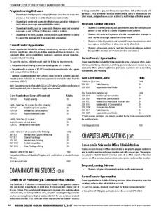
Open Ended Groups One problem arises when one or two values are a long way from the general mass of the data, either much lower or much higher. These values are called outliers. Their presence can mean having lots of empty or near-empty rows at one or both ends of the frequency table. For example, if one student is having weight of 24 kg in above example, then the groups (class intervals) 40-44, 35-39, 30-34 and 25-29 will have empty cells. In this case open-ended group can be used, here 0 asymmetric tail with more values above the mean - Skewness < 0 asymmetric tail with more values below the mean Skewned data is required to be treated using non parametric tests while normal curve data is treated using parametric tests. Kurtosis Kurtosis is a property associated with a frequency distribution and refers to the shape of the distribution of values regarding its relative flatness and peakedness. Compared with normal distribution, the interpretation of the kurtosis is: Kurtosis > 0 peaked relative to Normal distribution Kurtosis < 0 flat relative to Normal distribution Here are some examples of the shapes described above.

Shape of Distribution of Data

191

6

Peaked (Leptokurtic)

5 4

Normal (Mesokurtic)

3

Flatter ( Platykurtic) 2 1 0 0

2

4

6

8

10

Figure 11.8 Chart showing Kurtosis of distribution of data

Summary Shapes of data: 1. Uniform distribution 2. Positively skewed distribution 3. Negatively skewed distribution 4. Symmetric or Mound-shaped distribution 5. Bimodal or Multimodal distribution If the data is skewed it is required to be treated using non parametric tests while normal data is treated using parametric tests. Normal distribution: It is a bell shaped curve, symmetric and usually has Mean = Mode = Medium Skewness Skewness measures asymmetry around the mean. Kurtosis Kurtosis measures relative flatness and peakedness.

Multiple Choice Questions 1. If a distribution is skewed to the left, then it is __________. a. Negatively skewed b. Positively skewed c. Symmetrically skewed d. Symmetrical 2. If a test was generally very easy, except for a few students who had very low scores, then the distribution of scores would be _____. a. positively skewed b. negatively skewed c. not skewed at all d. normal


192

3. A measure of asymmetry is given by_________. a. kurtosis b. normal distribution c. skewness d. uniform distribution 4. A bell shaped distribution of data is said to be________. a. normal distribution b. positively skewed distribution c. negatively skewed distribution d. bimodel distribution 5. If the shape of distribution is flatter as compared to normal distribution, then the curve is _______. a. Leptokurtic b. Platykurtic c. Mesokurtic d. Skewed Exercise: 1. Describe shapes of data. 2. Write characteristics of normal distribution. 3. Why knowing the shape of the data is important? 4. Explain skewness with the help of diagram. 5. Explain kurtosis with the help of diagram. Answers: Multiple Choice Questions 1. a 2. b 3. c

4. a

5. b

Chapter 12

MEASURES OF CENTRAL TENDENCY Learning objectives When we have finished this chapter, we should be able to: 1. Explain what a summary measure of location is, and calculate the mode, median and mean for a set of values. 2. Demonstrate the role of data type and distributional shape in choosing the most appropriate measure of central tendency. 3. Explain what a percentile is, and calculate any given percentile value. 4. Explain what a summary measure of spread is, and calculate, the range, the interquartile range and the standard deviation. 5. Estimate percentile values from an ogive. 8. Demonstrate the role of data type and distributional shape in choosing the most appropriate measure of spread. 9. Draw a boxplot and explain how it works. 10. Explain the use of Excel in estimating all measures of central tendency. Introduction As we have seen in the previous two chapters, we can ‘describe’ raw data by charting it, or arranging it in table form or we can examine its shape. These procedures helps us to see patterns in the data. However, it is often more useful to summarise the data numerically. There are two principal features of a set of data that can be summarised with a single numeric value: 1. Measure of Location: A value around which the data has a tendency to congregate or cluster, is called as summary measure of location. 2. Measure of Dispersion: A value which measures the degree to which the data are spread out is called a summary measure of spread or dispersion. With these two summary values we can compare different sets of data quantitatively. Summary measures of location A summary measure of location is a value around which most of the data values tend to congregate or centre. Let us discuss three measures of location: the mode; the median; and the mean. 1. The Mode The mode is that category or value in the data that has the highest frequency (i.e. it occurs most often).The mode is not particularly useful with metric continuous data where no two values are

193


194

same. The other shortcoming of this measure is that there may be more than one mode in a set of data. 1. Mode for Ungrouped data Example 12.1 Calculate mode for ungrouped data given below 6, 8, 9, 7, 12, 3, 2, 4, 8, 1, 8, 5 Solution 1. First arrange the data in ascending order 1, 2, 3, 4, 5, 6, 7, 8, 8, 8, 9, 12. 2. Mode is frequently occuring value. In this example 8 is frequently occuring and hence mode is 8. 2. Mode for grouped data The mode for grouped data can be calculated by using the formula

æ f1 - f 0 ö ÷÷ ´ i Mode = l1 + çç è 2f1 - f 0 - f 2 ø Where, l1 = Lower limit of modal class

...1

f1 = Frequency of modal class f0 = Frequency before the modal class f2 = Frequency after the modal class i = Class interval of modal class Example 12.2 Calculate mode for following grouped data Table 12.1 Frequency distribution of Sales Per day Sales volume (Class interval) Number of days (Frequency)

53-56 2

57-60 4

61-64 5

65-68 4

69-72 4

72 and above 1

Solution Since the largest frequency corresponds to the class interval 61-64, hence it is the modal class. l1 = Lower limit of modal class = 61; f1 = Frequency of modal class = 5; f0 = Frequency before the modal class = 4; i = Class interval of modal class = 3 Formula æ f1 - f 0 ö ÷÷ ´ i Mode = l1 + çç è 2f1 - f 0 - f 2 ø

f2 = Frequency after the modal class = 4

Measures of Central Tendency

195

æ 5- 4 ö Mode = 61 + ç ÷ ´ 3 = 62.5 è 10 - 4 - 4 ø Hence, the modal sale is of 62.5 units. Example 12.3 Calculate mode for following grouped data Table 12.2 Frequency distribution for the heights of the Pharmacy students Height (inches) Frequency

57-59 47

59-61 23

61-63 65

63-65 51

65-67 20

67-69 08

Solution Since the largest frequency corresponds to the class interval 61-63, hence it is the modal class. l1 = Lower limit of modal class = 61; f1 = Frequency of modal class = 65; f0 = Frequency before the modal class = 23; f2 = Frequency after the modal class = 51 i = Class interval of modal class = 2 Formula æ f1 - f 0 ö ÷÷ ´ i Mode = l1 + çç è 2f1 - f 0 - f 2 ø

æ 65 - 51 ö Mode = 61 + ç ÷ ´ 2 = 61.5 è 130 - 23 - 51 ø Hence, the modal height is of 61.5 inches. 2. The Median If we arrange the data in ascending order of size, the median is the middle value. Thus, half of the values will be equal to or less than the median value, and half will be equal to or above it. The median is thus a measure of central-ness. If we have an even number of values, the median is the average of the two values either side of the ‘middle’. An advantage of the median is that it is not much affected by skewness in the distribution, or by the presence of outliers. However, it discards a lot of information, because it ignores most of the values, apart from those in the centre of the distribution. 1. Median for ungrouped data In this case the data is arranged in either ascending or descending order of magnitude. If the number of observations (n) is an odd number, then the median is represented by the numerical value corresponding to (n+1)/2th ordered observation.

196


æ n +1ö Median = Size or value of ç ÷ th observation ...2 è 2 ø If the number of observations (n) is an even number, then the median is defined as the arithmetic mean of the numerical values of n/2th and (n/2 + 1)th observations in the data array. n ö æn th + ç + 1÷ th observation 2 2 ø è ...3 Median = 2

Example 12.4 Calculate the median of the following data that relates to the number of patients per day in the outpatient ward in a Civil Hospital. 100, 200, 120, 170,130, 150, 180. Solution: 1. First arrange the data in an ascending order 100, 120, 130, 150, 170, 180, 200. 2. Since the number of observations in the data array are odd (n=7), the median for this data is æ n +1ö Median = Size or value of ç ÷ th observation è 2 ø æ 7 +1ö Median = ç ÷ = 4th observation è 2 ø

4th observation in the data array = 150. Thus the median number of patients examined per day in OPD in a Civil Hospital are 150. Example 12.5 Calculate the median of the following data that relates to the sale in lakh per month of a company in last one year. 12, 18, 15, 14, 13, 12, 20, 10, 11, 18, 19, 16 Solution: 1. First arrange the data in ascending order 10, 11, 12, 12, 13, 14, 15, 16, 18, 18, 19, 20. 2. Since the number of observations in the data array are even (n=12), the median for this data is n æn ö th + ç + 1÷ th 2 è2 ø Median = 2 12 æ 12 ö th + ç + 1÷th 2 è2 ø = (6th value + 7th value) = 14 + 15 = 14.5 Median = 2 2 2

Thus the median sale of company per month is 14.5 lakhs.


197

2. Median for grouped data (Metric continuous) To find the median for grouped data, first we need to identify the class interval which contains the median value or (n/2)th observation of the data set. To identify such class interval, we should find the cumulative frequency of each class until the class for which the cumulative frequency is equal to or greater than the value of (n/2)th observation. The value of the median within that class is found by using interpolation. It is assumed that the observation values are evenly spaced over the entire class interval. The following formula is used to determine the median of grouped data:

Median = l1 +

(n/2) - c.f. ´ i f

...4

Where l1 = Lower limit of median class. c.f. = Cumulative frequency of the class prior to the median class. f = Frequency of median class. i = Class interval of median class. th

Median class is the class in which n/2 observation lies. To use above formula, data should be continuous. Example 12.6 A survey was conducted to determine the age (in years) of 130 pharmacists. The result of such a survey is as follows: Table 12.3 Frequency distribution of age of Pharmacist Age of pharmacist Number of Pharmacist

20-25 6

25-30 13

30-35 29

35-40 48

40-45 22

45-50 8

50-55 4

Solution: First, we should find the cumulative frequencies to locate the median class ( see table 12.4). Table 12.4 Calculations for median age of pharmacist Age of pharmacist (in years)

No of pharmacist (f)

Cumulative frequency (cf)

20-25 25-30 30-35 35-40 40-45 45-50 50-55

06 13 29 48 22 08 04 n=130

06 19 48 96 118 126 130

Median class


198

Here the total number of observations are n = 130. Median is the size of (n/2)th = 130/2 = 65th observation in the data set. This observation lies in the class interval 35-40. l1 = Lower limit of median class = 35 c.f.= Cumulative frequency of the class prior to the median class interval = 48 f = Frequency of median class = 48 i= Class interval of median class = 5 Formula (n/2) - c.f. Median = l1 + ´ i f (130/2) - 48 17 Median = 35 + ´ 5 = 35 + ´ 5 = 35 + 1.77 = 36.77 48 48 Hence the median age of pharmacist is 36.77 years. Example 12.7 A survey was conducted to determine the height (in inches) of 50 pharmacists. The result of such a survey is as follows: Table 12.5 Frequency distribution of age of Pharmacist Height of pharmacist Number of Pharmacist

44-48 1

48-52 2

52-58 7

58-62 8

62-66 18

66-70 12

70-74 2

Solution: First, we should find the cumulative frequencies to locate the median class ( see table 12.6). Table 12.6 Calculations for median age of pharmacist Height of pharmacist (in inches)

44-48 48-52 52-58 58-62 62-66 66-70 70-74

No of pharmacist (f)

01 02 07 08 18 12 02 n=50


01 03 10 18 36 48 50

Median class

Here the total number of observations are n = 50. Median is the size of (n/2)th = 50/2 = 25th observation in the data set. This observation lies in the class interval 62-66. l1 = Lower limit of median class = 62


199

c.f.= Cumulative frequency of the class prior to the median class interval = 18 f= Frequency of median class = 36 i= Class interval of median class = 4

(n/2) - c.f. í f (50/2) - 18 Median = 62 + ´ 4 = 62.78 36

Median = l1 +

Hence the median age of pharmacist is 62.78 inches. 3. Median for Metric Discrete data Median for metric discrete data is calculated as follows Median = value of (n/2)th observation Example 12.8 The information on the number of defective components in 1000 boxes, is given below Table 12. 7 Data of number of defective components in 1000 boxes No. of defective components 0 Number of boxes 25

1 306

2 402

3 200

4 51

5 10

6 6

Calculate the median of defective components for the whole of the production line. Solution For the calculation of median defective components for the whole production line the frequency table as shown in table 12.8 is required. Table 12.8 Frequency table for calculation of median for Metric discrete data No. of defective components

No. of Boxes (f)


0 1 2 3 4 5 6

25 306 402 200 51 10 06 n = 1000

25 331 733 933 984 994 1000

Median = value of (n/2)th observation = value of (1000/2) th observation = value of 500th observation

200


In cumulative frequency column 500th observation comes after 331 and before 733. Hence median is 2 defective components. 3. The Mean The mean, or the arithmetic mean, is more commonly known as the average. One advantage of the mean over the median is that it uses all of the information in the data set. However, it is affected by skewness in the distribution, and by the presence of outliers in the data. This may, sometimes, produce a mean that is not very representative of the general mass of the data. Moreover, it cannot be used with ordinal data (as ordinal data are not real numbers, so they cannot be added or divided). 1. Mean for Ungrouped data The mean of ungrouped data is calculated by adding the values of all observations and dividing the total by the number of observations. Mean ( X ) =

Sum of all observations ( å X) Total number of observations (N)

...5

Example 12.9 The following data gives weight of 20 paracetamol tablets in mg. Calculate average weight of a paracetamol tablet. 625, 617, 633, 630, 620, 631, 618, 620, 619, 632, 625, 628, 626, 624, 622, 625, 627, 631, 619, 624. Solution: Mean (X) =

Sum of all observations (å X) 12496 = = 624.8 Total number of observations (N) 20

Hence mean weight of paracetamol tablet is 624.8. Example 12.10 The blood serum cholesterol levels of 10 subjects are given as: 245 262 292 247 253 286 274 265 Calculate mean. Solution: Mean (X ) =

Sum of all observations (å X) 2655 = = 265.5 Total number of observations (N) 10

Hence mean cholesterol levels of 10 subject is 265.5.

279

252


201

2. Mean for metric continuous data (grouped data) Mean for metric continuous grouped data can be calculated by using following formula å fd ´ i Mean ( X ) = A + ...6 N Where A=Assumed mean f = frequency of ith class interval N = Summation of all frequencies d = (mi -A)/ i, deviation from assumed mean m = mid value of ith class interval i = width of the class interval Example 12.11 A company is planning to improve plant safety. For this, accident data for the last 50 weeks was compiled. These data are grouped into the frequency distribution as shown below. Calculate mean of the number of accidents per week. Table 12.9 Number of accidents in last 50 weeks No. of accidents Number of weeks

0-4 5

5-9 22

10-14 13

15-19 8

20-24 2

Solution 1. Construct frequency distribution table as per given in table 12.10. Table 12.10 Calculations for mean accidents per week No. of Accidents class interval

0-4 5-9 10-14 15-19 20-24

No of weeks (f)

5 22 13 8 2 N= 50

Mid value of class interval (m)

Deviation from assumed mean (d )

02 07 12 17 22

-2 -1 0 1 2

A

fd

-10 -22 0 8 4 å fd = -20

2. Take the mid point of any class interval as assumed mean (A). Here we have taken the mid point of class interval of 10-14, which is 12, as assumed mean. 3. Set third column as d. That gives deviation from assumed mean, which is calculated by using formula: (mid point of ith class interval - assumed mean)/ width of class interval. Here class interval is 5.


202

4. Finally set forth column fd and calculate å fd. 5. Now put the values in formula for calculation of mean for grouped data Data: A=Assumed mean = 12 N = Summation of all frequencies = 50 åf d = -20 i = width of the class interval = 5 Formula:

Mean ( X ) = A +

å fd ´ i

Mean ( X ) = 12 +

N

- 20 ´ 5 = 10 50

Hence mean of the number of accidents per week is 10. Example 12.12 The following are the weights in kg of 60 final year pharmacy students. Calculate mean weight. Table 12.11 Weights of 60 final year students Weight (kg) Frequency

45-49 50-54 3 10

55-59 12

60-64 15

65-69 6

70-74 7

75-79 5

80-54 2

Solution 1. Construct frequency distribution table as per given in table 12.12. Table 12.12 Calculations for mean weight of final year students Weight ( kg)

Frequency n=60

Mid value of class interval (m)

45-49 50-54 55-59 60-64 65-69 70-74 75-79 80-84

03 10 12 15 06 07 05 02 N= 60

47 52 57 62 67 72 77 82

A

Deviation from assumed mean (d)

-3 -2 -1 0 1 2 3 4

fd

-9 -20 -12 0 6 14 15 8 å fd = 2


203

2. Take the mid point of any class interval as assumed mean (A). Here we have taken the mid point of class interval of 60-64, which is 62, as assumed mean. 3. Set third column as d. That gives deviation from assumed mean, which is calculated by using formula: (mid point of ith class interval - assumed mean)/ width of class interval. Here class interval is 5. 4. Finally set forth column fd and calculate å fd. 5. Now put the values in formula for calculation of mean for grouped data Data: A=Assumed mean = 62 N = Summation of all frequencies = 60 åf d = 2 i = width of the class interval = 5 Formula: åf d í Mean ( X ) = A + N 2 Mean ( X ) = 62 + ´ 5 = 62 .16 60 Hence mean weight of final year pharmacy students is 62.16 kg. 3. Mean for Metric Discrete data (frequency data) When observations are grouped as a frequency distribution, then mean is calculated by using following formula:

Mean (X) =

åf X i

i

...7

N

Where N = å fi fi = frequency with which variable Xi occurs Example 12.13 Following data gives number of times that inhaler used in past 24h by 53 children with asthma. Find mean number of times inhaler used by children with asthma. Table 12.13 Number of times inhaler used by children No. of times inhaler used Number of children

0 6

1 16

2 12

3 8

4 5

5 3

6 2

7 1


204

Solution: 1. Construct frequency distribution table as per given in table 12.14. 2. Set third column as fiXi. 3. Determine summation of fi and fiXi. 4. Now put the values in formula for calculation of mean for grouped discrete data Table 12.14 Calculation of mean for metric discrete data Number of children (fi)

Number of times inhaler used in past 24 h (Xi)

0 1 2 3 4 5 6 7

06 16 12 08 05 03 02 01 N= åfi = 53

fiXi

0 16 24 24 20 15 12 7 å fiXi = 118

Applying formula 7, the mean is

Mean (X) =

åf X i

N

i

=

118 = 2.23 53

Hence mean number of times inhaler used by children with asthma in past 24 h was 2.23. Example 12.14 Calculate mean number of living children per woman from the following table. Table 12.15 Number of living children per woman No. of living children Number of women

0 42

1 49

2 57

3 40

4 31

5 22

Solution: 1. Construct frequency distribution table as per given in table 12.16. 2. Set third column as fiXi. 3. Determine summation of fi and fiXi. 4. Now put the values in formula for calculation of mean for grouped discrete data.


205

Table 12.16 Calculation of mean for metric discrete data Number of Women (fi)

Number of living children (Xi)

0 1 2 3 4 5

42 49 57 40 31 22 N= åfi = 241

fiXi

0 49 114 120 124 110 å fiXi = 517

Applying formula 7, the mean is

Mean (X) =

åf X i

N

i

=

517 = 2.145 241

Hence mean number of living children per woman was 2.145. Choosing the most appropriate measure The most appropriate measure of location for given set of data is given below in the table 12.10. The main thing to remember is that the mean cannot be used with ordinal data (because they are not real numbers), and that the median can be used for both ordinal and metric data (particularly when the latter is skewed). Table 12.17 Aguide to choosing an appropriate measure of location Type of variable

Nominal Ordinal Metric continuous Metric discrete

Mode

yes yes yes yes

Summary measure of location Median

no yes yes, if skewed yes, if skewed

Mean

no no yes yes

4. Percentiles The measures of central values discussed so far are averages. They locate the centre or mid point of a distribution. It may also be of interest to locate other points in the range like percentiles. They are values of a variable which divide the total observations by an imaginary line into two parts, expressed in percentages such as 10% and 90% or 25% and 75%, etc. In all, there are 99 percentiles. Percentiles are values in a series of observations arranged in ascending order of magnitude which divide the distribution into 100 equal parts. Thus, the median is 50th percentile. The 50th percentile


206

will have 50% observations on either side. Accordingly, 10th percentile will have 10% observations to the left and 90% to the right. Quartiles are three different points located on the entire range of a variable- Q1, Q2 and Q3. Q1 or lower quartile will have 25% observations falling on its left and 75% on its right: Q2 or median will have 50% observations on either side and Q3 or upper quartile will have 75 % observations on its left and 25% on its right. Quintiles are four in number and divide the distribution into 5 equal parts. So 20th percentile or first quintile will have 20% observations falling to its left and 80% to its right. Deciles are nine in number and divide the distribution into 10 equal parts, first decile or 10th percentile will divide the distribution into 10% and 90% while 9th decile will divide into 90% and 10% . Calculating a percentile value Percentile value is calculated by using formula Pth Percentile =

P (N + 1)th value 100

...8

Where P = percentile N = number of values Example 12.15 Following table records the percentage mortality in 26 ICUs. Calculate the 25th and 75th percentiles for the ICU percent mortality values. Table 12.18 Percent mortality in 26 ICUs ICU 1 % mortality 15.2

2 3 31.3 14.9

4 5 6 7 8 9 10 16.3 19.3 18.2 20.2 12.8 14.7 29.4

11 21.1

12 20.4

13 13.6

ICU 14 % mortality 22.4

15 14

16 17 18 19 20 21 22 23 14.3 22.8 26.7 18.9 13.7 17.7 27.2 19.3

24 16.1

25 13.5

26 11.2

Solution: 1. First, arrange values in ascending order for 26 ICUs as shown below 1 ICU % mortality 11.2

2 3 4 5 6 12.8 13.5 13.6 13.7 14

ICU 14 15 16 17 % mortality 18.2 18.9 19.3 19.3 th

7 8 9 10 14.3 14.7 14.9 15.2

11 16.3

12 16.1

13 17.7

18 19 20 21 22 23 20.2 20.4 21.1 22.4 22.8 26.7

24 27.2

25 29.4

26 31.3

2. Now, the 25 percentile can be calculated by using formula


Pth Percentile =

207


P= 25th percentile = 25 N= no. of ICU = 26 25 th Percentile =

25 (26 + 1) = 0.25 ´ 27th value = 6.75th value 100

th

th

The 6 value is 14 % while the 7 value is 14.3%, A difference is of 0.3, th

The 25 percentile is 14% + 0.75 of 0.3, 14% + 0.75 x 0.3% = 14% + 0.225 =14.225 th So, the 25 percentile for the ICU percent mortality is 14.225.

th

3. Now, the 75 percentile can also be calculated using same formula, P = 75 and N = 26. 75th Percentile = th

75 (26 + 1) = 0.75 ´ 27th value = 20.25th value 100 st

The 20 value is 21.1 % while the 21 value is 22.4%, a differences of 1.3, The 75th percentile is 21.1% + 0.25 of 1.3 = 21.1% + 0.25 x 1.3% = 21.1% + 0.325 =21.425 So, the 75th percentile for the ICU percent mortality is 21.425. Summary measures of spread There are three main measures of spread or dispersion in common use. Here also, the type of data influences the choice of an appropriate measure. 1. The Range The range is the distance from the smallest value to the largest. The range is not affected by skewness, but is sensitive to the addition or removal of an outlier value. Range = Lowest value to Highest value. ...9 Example 12.16 Weight of six paracetamol tablets in mg are given below. Find weight range for paracetamol tablet. Data: 625, 612, 615, 632, 628, 618 Solution: 1.Arrange data in ascending order 612, 615, 618, 625, 628, 632 2. Lowest value = 612 mg 3. Highest value = 632 mg


208

Range is 612 to 632 mg. 2. The interquartile range (iqr) One solution to the problem of the sensitivity of the range to extreme value (outliers) is to chop a quarter (25 per cent) of the values off both ends of the distribution, which removes any troublesome outliers, and then measure the range of the remaining values. This distance is called the interquartile range, or iqr. The interquartile range is not affected either by outliers or skewness, but it does not use all of the information in the data set since it ignores the bottom and top quarter of values. Calculating interquartile range To calculate the interquartile range, first we need to determine two values: 1. The value which cuts off the bottom 25th percentile of values; this is known as the first quartile and denoted as Q1. 2. The value which cuts off the top 75th percentile of values, known as the third quartile and denoted as Q3. The interquartile range is then written as (Q1 to Q3). Example 12.17 Calculate the iqr for the ICU percentage mortality values in table 12.19 . Table 12.19 Percent mortality in 26 ICUs 1 ICU % mortality 15.2

2 3 31.3 14.9

4 5 6 7 8 9 10 16.3 19.3 18.2 20.2 12.8 14.7 29.4

11 21.1

12 20.4

13 13.6

ICU 14 % mortality 22.4

15 14

16 17 18 19 20 21 22 23 14.3 22.8 26.7 18.9 13.7 17.7 27.2 19.3

24 16.1

25 13.5

26 11.2

Solution 1.Arrange the data in ascending order 2. Calculate 25th percentile as a Q1 3. Calculate 75th percentile as a Q3 4. We have already calculated the 25th and 75th percentiles before in example 12.15 Q1 = 14.225%, Q3 = 21.425% Therefore interquartile range = (14.225 to 21.425) %. Estimating the median and interquartile range from Ogive We can also estimate interquartile range from ogive. If we draw horizontal lines from the values 25 per cent, 50 per cent and 75 per cent on the y axis, to the ogive, and then down to the x axis, the points of intersection on the x axis approximately gives values for Q1, Q2 (the median), and Q3.


209

Example 12.18 Estimate iqr for the data of weight in kg of 60 final year pharmacy students given in Table 10.6. Table 12.20 Weights of 60 final year students Weight (kg) Frequency

45-49 50-54 3 10

55-59 12

60-64 15

65-69 6

70-74 7

75-79 5

80-54 2

% Relative cumulative frequency

Solution We have already drawn ogive of this example. Ogive is drawn by plotting % cumulative frequency on Y axis against midpoint of class interval on X axis. Now, draw perpendicular to ogive at 25th percentile (Q1), 50th percentile (Q2) and 75th percentile (Q3) as shown in figure below. 100

Q3= 66

75

Q2= 58.5

50

Q1= 53

25

0 40

50 60 70 Mid point of class interval

80

90

Figure 12.1 % cumulative frequency curve of weight to estimate median and iqr The weight values corresponding to these perpendiculars are taken as Q1, Q2 and Q3 and here they are Q1=53, Q2 = 58.5 and Q3 =66 Interquartile range (IQR)= Q1 to Q3 Interquartile range (IQR)= 53 to 66 The interquartile range for the data of weights of final year students is 53 to 66 kg. The Boxplot Now that we have discussed the median and interquartile range, we can now better understand the boxplot which we had seen in chapter 11. Boxplots provide a graphical summary of the three quartile values, the minimum and maximum values, and any outliers. They are usually plotted with value on the vertical axis. Like the pie chart, the boxplot can only represent one variable at a time, but a number of boxplots can be set alongside each other.


210

Let’s understand the boxplot, 1. The bottom end of the lower ‘whisker’(the line sticking out of the bottom of the box), corresponds to the minimum value. 2. The bottom of the box is the 1st quartile value, Q1. 3. The line across the inside of the box, is the median, Q2. The median line will always not be at the centre. The more asymmetric (skewed) the distributional shape, the median line will be further away from the middle of the box. If it is closer to the top of the box, it indicates negative skew while if it is closer to the bottom of the box, it indicates positive skew. 4. The top of the box is the third quartile Q3. 5. The top end of the upper whisker is the ‘maximum’. This is the maximum value that can be considered still to be part of the general mass of the data. 6. There is one outlier. This is, the actual maximum value in the data.

Percentage of label claim

120

110

100

90

80

n = 50 Figure 12.1 Boxplot

Example 12.21 Sketch the box plot for the percentage mortality in ICUs shown in table 12.10. We have already calculated Q1 and Q3 for same. Solution: Calculation of Q2, Median The 50th percentile can be calculated using formula

Pth Percentile = th


P = 50 percentile = 50; N = 26


211

50 (26 + 1) = 0.5 ´ 27th value = 13.5th value 100 The 13th value is 17.7 % while the 14th value is 18.2%. A differences of 0.5.

50th Percentile =

The 50th percentile is 17.7% + 0.5 of 0.5 = 17.7% + 0.5 x 0.5% = 17.7% +0.25 =17.95 So, the 25th percentile for the ICU percent mortality is 14.225. So, the 50th percentile for the ICU percent mortality is 17.95. So, the 75th percentile for the ICU percent mortality is 21.425. Now, the box plot can be sketched as under

Maximum

75th percentile 50th percentile 25th percentile

Minimum

Figure 12.2. Box plot for percentage mortality in ICUs 3. Standard Deviation and Variance The limitation of the interquartile range as a summary measure of spread is that, it is not using all the information in the data, since it omits the top and bottom quarter of values. An alternative approach we can use is to measure the mean (average) distance of all the data values from the overall mean of all of the values. The smaller this mean distance is, the narrower the spread of values will be, and vice versa. This approach is known as the standard deviation, or s.d. Standard deviation can be calculated by using following steps: 1. Subtract the mean of the sample from each of the n sample values in the sample, to give the difference values. 2. Square each of these differences. 3. Add these squared values together (called the sum of squares). 4. Divide the sum of squares by (N – 1); i.e. divide by 1 less than the sample size. 5. Take the square root. This is the standard deviation Variance is the square of standard deviation and is used instead of standard deviation. Example 12.23 A microbiologist found 8, 10, 19, 12, 6 and 5 E. coli in six culture. Calculate standard


212 2

deviation, s and variance, s . Solution 1. Let us calculate the mean

8 + 10 + 19 + 12 + 6 + 5 = 10 6 2. Now, construct the table as shown below: Mean, X =

(x - `x ) -2 0 9 2 -4 -5

x 08 10 19 12 06 05

(x - `x )2 4 0 81 04 16 25

å(x - `x )2=130 3. Let us use å(x - `x ) value in the formula Formula 2

Standard deviation (s) =

å(X - X) 2 N -1


130 = 26 = 5.1 6 -1

...10

2

4. Thus, standard deviation, s was found to be 5.1 while variance, s was found to be 26. However, the calculations using this formula can be tedious when the numbers and mean are in decimals. So, the computing formula used is as follows Formula (å X)2 å X2 N ...11 Standard deviation (s) = N -1 Let us calculate standard deviation using this formula x 08 10 19 12 06 05 åx = 60

2

x 64 100 361 144 36 25 åx =730 2


213

Hence: N = 6, åX = 60, åX =730 2


(60) 2 10 = 5.1 6 -1

730 -

2

The, standard deviation, s by this method is also 5.1 and variance, s is 26. 1. Standard deviation (s) in ungrouped data For calculation of standard deviation in ungrouped data following formula is used, where assumed mean method is used so that squaring of large values can be avoided.


(å X )2 N N -1

å X2 -

... 12

Where, N = number of observations X = deviation from assumed mean = x-A. A=Assumed mean x = given observations Example 12.23 Find standard deviation of incubation period of smallpox in 9 patients where it was found to be 14, 13, 11, 15, 10, 7, 9, 12, and 10. Solution 1. Construct calculation table as per given in table no 12.21. 2. Set any assumed mean from set of observations (x). 3. Set second column as deviation from assumed mean i.e. X=x-A. 4. Set third column as square of deviation i.e X

2 2

5. Determine summation of deviation from assumed mean (X) and square of deviation (X ). 6. Finally put the values in equation 10 so as to get standard deviation for ungrouped data.


214

Table 12.21 Calculation of standard deviation for ungrouped data Incubation period of smallpox (x)

14 13 11 15 10 7 9 12 10

Deviation from assumed mean (X= x - 11)

3 2 0 4 -1 -4 -2 1 -1 åX = 2

A

Data

Square of deviation X2

9 4 0 16 1 16 4 1 1 2 åX = 52

N=9 Summation of deviation from assumed mean, X =2 2

Summation of square of deviation, X = 52 Formula (å X)2 å X2 N Standard deviation (s) = N -1

22 9 = 9 -1

52 Standard deviation (s) =

51.56 = 8

6 .443 = 2.54

Therefore, standard deviation of incubation period of smallpox in 9 patients was 2.54. Example 12.24 The following data gives weight of 10 paracetamol tablets in mg. Find standard deviation. 625 617 633 630 620 631 618 620 619 632 Solution 1. Construct calculation table as per given in table no 12.22. 2. Set any assumed mean from set of observations (x). 3. Set second column as deviation from assumed mean i.e. X=x-A. 2

4. Set third column as square of deviation i.e X

2

5. Determine summation of deviation from assumed mean (X) and square of deviation (X ). 6. Finally put the values in equation 10 so as to get standard deviation for ungrouped data.


215

Table 12.22 Calculation of standard deviation for ungrouped data Weight of Paracetamol tablets (x)

625 617 633 630 620 631 618 620 619 632

Deviation from assumed mean (X= x - 625)

Square of deviation X2

0 -8 8 5 -5 6 7 -5 -6 7

0 64 64 25 25 36 49 25 36 49

åX= -5

åX = 373

A

2

Data N = 10 Summation of deviation from assumed mean, X = -5 2

Summation of square of deviation, X = 373 Formula (å X) 2 å X2 N Standard deviation (s) = N -1


- 52 10 = 6.416 10 - 1

373 -

Therefore, standard deviation of weight of 10 paracetamol tablets was 6.416. 2. Standard deviation (s) in grouped data Standard deviation in grouped data is calculated by using formula:


( å fd ) 2 N í N -1

å fd 2 -

Where, f = frequency N = summation of frequency, f = Sf

...13


216

d = (m.p. - A)/ i m.p. = mid point A=Assumed mean i = class interval Example 12.25 Calculate SD of following data Table 12.23 IQ of 50 students IQ 0-20 Number of students 3

20-40 4

40-60 3

60-80 4

80-100 13

100-120 12

120-140 8

140-160 3

Answer: 1. Construct calculation table as per given in table no 12.24. 2. Construct third column as mid value of class interval. 3. Set any assumed mean (A) from set of mid points (m.p.). 4. Set forth column as deviation from assumed mean i.e.d= (m.p. -A)/ i. 2

5. Determine fd and fd . 2

6. Determine summation of f, fd and fd . 7. Finally put the values in equation 11 so as to get standard deviation for grouped data. Table 12.24 Calculation of SD in grouped data No of Students (f)

IQ

0-20 20-40 40-60 60-80 80-100 100-120 120-140 140-160

Mid value of class interval (m.p.)

3 4 3 4 13 12 8 3

N=Sf = 50 Data: Class interval, i = 20; Assumed mean, A= 90; N=Sf = 50; Sfd=3;

10 30 50 70 90 110 130 150

A

d (mp - A)/i

-4 -3 -2 -1 0 1 2 3

d

2

16 9 4 1 0 1 4 9

fd

f d2

-12 -12 -6 -4 0 12 16 9

48 36 12 4 0 12 32 9

Sfd=3 Sfd2= 171


Sfd = 171 Formula:

217

2


( å fd ) 2 N í N -1

å fd 2 -

Solution: Now, putting the values in above formula, we get

( 3) 2 50 ´ 20 = 3.48 ´ 20 = 37 .2 Standard deviation (s) = 50 - 1 Therefore standard deviation of given IQ data is 37.2. 171 -

Example 12.26 Calculate SD of following data of intelligence quotient (IQ) of 50 students. Table 12.25 Given data Classes Frequency

0-10 5

10-20 10

20-30 15

30-40 20

40-50 25

50-60 12

60-70 8

70-80 4

80-90 1

Answer: 1. Construct calculation table as per given in table no 12.26. 2. Construct third column as mid value of class interval. 3. Set any assumed mean (A) from set of mid points (m.p.). 4. Set forth column as deviation from assumed mean i.e. d= (m.p. -A)/ i. 2

5. Determine fd and fd . 6. Determine summation of f, fd and fd2. 7. Finally put the values in equation 11 so as to get standard deviation for grouped data. Table 12.26 Calculation of SD in grouped data 2 Frequency Mid value of Classes d d fd f d2 (f) class interval (m.p.) (mp - A)/i 0-10 5 5 -4 16 -20 80 10-20 10 15 -3 9 -30 90 20-30 15 25 -2 4 -30 60 30-40 20 35 -1 1 -20 20 A 40-50 25 45 0 0 0 0 50-60 12 55 1 1 12 12 60-70 8 65 2 4 16 32 70-80 4 75 3 9 12 36 80-90 1 85 4 16 4 16 2 Sfd=-56 Sfd = 346 N=Sf = 100


218

Data: Class interval, i = 10; Assumed mean, A= 45; N=Sf = 100; Sfd=-56; Sfd = 346 Formula: 2

( å fd ) 2 N N -1

å fd 2 -


í

Solution: Now, putting the values in above formula, we get

( - 56 ) 2 100 ´ 10 = 17.8 100 - 1

346 -


Therefore standard deviation of given data is 17.8. 3. Standard deviation in metric discrete data Standard deviation for metric discrete data is given by the formula:

(å f i X i ) 2 N N -1

å fiXi 2


...14

Where, fi = frequency with which variable Xi occurs N = åfi Example 12.27 Calculate standard deviation of Example 12.13 No. of times inhaler used Number of children

0 6

1 16

2 12

3 8

4 5

5 3

6 2

7 1


219

Solution 1. Construct the frequency table as shown below: Number of children Number of times inhaler used in past 24 h fiXi (fi) (Xi) 0 06 0 1 16 16 2 12 24 3 08 24 4 05 20 5 03 15 6 02 12 7 01 7 N= åfi = 53 å fiXi = 118

Xi2

fiXi2

0 0 1 16 4 48 9 72 16 80 25 75 36 72 49 49 2 åfiXi = 412

Data N= åfi = 53 å fiXi = 118 åfiXi2 = 412 Formula 2


(å fiX i )2 N N -1

å fiX i -

2. Now put the values in the formula


(118 ) 2 53 = 53 - 1

412 -

412 - 262.71 = 1.72 53 - 1

So, the standard deviation was found to be 1.72. Measurement related to sample standard deviation The variability of data may often be better described as a relative variation rather than as an absolute variation (i.e., the standard deviation). This can be accomplished by calculating the coefficient of variation (CV) that is the ratio of the standard deviation to the mean. SD ...15 Coefficient of variation (CV) = mean The CV is usually expressed as a percentage (relative standard deviation or RSD) and can be useful in many instances because it places variability in perspective to the distribution center. Relative Standard Deviation = CV x 100 ...16

220


Example 12.28 In two series of adults aged 21 years and children 3 months old, following values were obtained for the height. Find which series shows greater variation? Persons Mean height SD Data Adults 160 cm 10 cm Children 60 cm 5 cm Formula: CV = SD/mean RSD = CV x 100 Solution: Put the values in equation Adults CV of adults = 10/160 = 0.0625 RSD = 0.0625 x 100 = 6.25 % Children CV of children = 5/60 = 0.0833 RSD = 0.0833 x 100 = 8.33 % Thus, heights in children show greater variation than adult. Example 12.29 Chest circumference in cm of 10 malnourished children and normal children aged one year, are given below. Find which series shows greater variation? Data Children Mean height SD Malnourished 48.5 4.53 Normal 34.8 4.57 Formula: CV = SD/mean RSD = CV x 100 Solution: Put the values in equation Malnourished CV = 4.53/48.5 = 0.09 RSD = 0.093 x 100 = 9.3 % Normal CV = 4.57/34.8 = 0.131 RSD = 0.131 x 100 = 13.1 % Thus, Normal children show greater variation than malnourished children.


221

Choosing an appropriate measure of spread Table 12.27 Choosing an appropriate measure of spread Type of variable

Nominal Ordinal Metric

Range

no yes yes

Summary measure of spread Interquartile range

no yes yes, if skewed

Standard deviation

no no yes

Use of Excel in Measures of Central Tendency We can easily calculate both measures of central tendency i.e measures of location and measures of dispersion in excel where we need not have to worry about any formulas. Excel will readily calculate these values for us. So, lets see how we can use excel for calculating measures of central tendency. Installing theAnalysis ToolPak in Excel Excel includes a number of add-in tools to assist with a number of data handling, reporting and analysis functions. So, first we will install this analysis toolpak as given below: 1. Open New workbook from MS-Excel and click to Tools menu from Menu bar. 2. Instantly, it will display pull-down menus. 3. Select onAdd-Ins option. 4. In the Manage box, selectAdd-ins-Analysis ToolPak as shown in figure. 6. Then, click on OK button. This unpacks the chosen Excel Add-in tools and makes them available for use. If the Add-in list is empty, there may have been a limited installation of MS Office. In this case, the MS Office CDs will be needed to install theseAdd-in tools.

Figure 12.3 Window of Add-Ins

222


Use of Excel in Descriptive Statistics The Data Analysis ToolPak has a Descriptive Statistics tool that provides us with an easy way to calculate summary statistics for a set of sample data. Summary statistics includes Mean, Standard Error, Median, Mode, Standard Deviation, Variance, Kurtosis, Skewness, Range, Minimum, Maximum, Sum, and Count. This tool eliminates the need to type individual functions to find each of these results. Excel includes elaborate and customizable toolbars. We can follow the below steps: Step 1. Open New Excel file. In sheet 1 put labels in first row (i.e A1, B1) and enter the data below these labels. Step 2. Select the Tools menu from menu bar. Then, it will display pull-down menus. Step 3. Click on the data analysis option. Instantly, dialog box will appear. Step 4. Choose Descriptive Statistics from Analysis Tools list of Data Analysis dialog box. Lastly, click on OK button. This will display the Descriptive Statistics dialog box on the screen.

Figure 12.4 Window of Data Analysis Step 4. When the dialog box appears; Enter range of data or select range (along with labels) in the Input Range box. Tick mark on Labels in first row and summary statistics of Output options, as shown below: Note: Ensure that labels are given in first row. Step 5. Ignore remaining settings and click on Ok button.

Figure 12.5 Window of Descriptive statistics


223

Step 6. We will get result of descriptive statistics as shown below. Column1 Mean Standard Error Median Mode Standard Deviation Sample Variance Kurtosis Skewness Range Minimum Maximum Sum Count

Summary The mean, median and mode, are common measures of location which represent either a typical or representative score and/or a value about which the data tend to center. Mode The mode (denoted by M) represents the most frequently occurring score. When more than two scores occur with the greatest frequency, the data set is said to be multimodal. Mode for grouped data æ f1 - f 0 ö ÷÷ ´ i Mode = l1 + çç è 2f1 - f 0 - f 2 ø Median th

The median of a set of scores represents the middle value (50 percentile) when the scores are arranged as an array in order of increasing (or decreasing) magnitude. Median for ungrouped data Odd number æ n +1ö Median = Size or value of ç ÷ th observation è 2 ø Even number

n ö æn th + ç + 1 ÷ th 2 ø è2 Median = value of observation 2

Median for grouped data Median = l1 +

(n/2) - c.f. ´ i f

Median for Metric Discrete data Median = value of (n/2)th observation


224

Mean Mean represents the most appropriate measure of central tendency for continuous-type data. It is obtained by adding all of the scores and dividing this sum by the number of scores. Mean for ungrouped data Sum of all observations (å X) Mean (X) = Total number of observations (N) Mean for grouped data Mean ( X ) = A +

Mean for Metric Discrete data

Mean (X) =

å fd ´ i

åf X i

N

i

N

Percentile Percentiles are values in a series of observations arranged in ascending order of magnitude which divide the distribution into 100 equal parts. P Pth Percentile = (N + 1)th value 100 The range, interquartile range, standard deviation are common measures of spread and represents the extent of spread of data Range The range is the distance from the smallest value to the largest. Range = Lowest value to Highest value. The interquartile range The interquartile range is Q1 to Q3 Q1 is the value which cuts off the bottom 25th percent of values and is known as the first quartile (25th percentile),while Q3 cut off top 25th percent of values and is known as third quartile (75th percentile). Standard Deviation (SD) The standard deviation measures the variation of scores about the mean (average) score, and can be defined as the “root mean squared deviation.” Variance is square of standard deviation. Standard deviation of ungrouped data Standard deviation (s) =

(å X )2 N N -1

å X2 -

Standard deviation of grouped data Standard deviation (s) =

( å fd ) 2 N í N -1

å fd 2 -


225

Standard deviation for metric discrete data


(å f i X i ) 2 N N -1

å f i X i2 -

Measurement related to sample standard deviation Coefficient of variation (CV) =

SD mean

Relative Standard Deviation = CV x 100 Choosing an appropriate measure of central tendency Type of variable

Nominal Ordinal Metric

Summary measures of location Mode Mean Median

yes yes yes


no no yes

Summary measures of spread Range SD Iqr

no yes yes


no no yes

Multiple choice questions 1. The range of a sample gives an indication of the________. a. way in which the values cluster about a particular point b. number of observations bearing the same value c. maximum variation in the sample d. degree to which the mean value differs from its expected value. 2. The observation which occurs most frequently in a sample is the__________. a. median b. mean deviation c. standard deviation d. mode 3. What is the median of the sample 5, 5, 11, 9, 8, 5, 8 ? a. 5 b. 6 c. 8 d. 9 4. What is the median of the following set of scores? 18, 6, 12, 10, 14 ? a. 10 b. 14 c. 18 d. 12 5. All of the following are measures of central location except________. a. range b. arithmetic mean c. median d. mode 6. The measure of central location that has half of the observations below it and half of the observations above it is the__________. a. arithmetic mean b. geometric mean c. median d. mode 7. The most commonly used measure of central location is the________. a. mean b. range c. median d. mode

226


8.All of the following are measures of dispersion except______. a. interquartile range b. percentile c. variance d. standard deviation 9. The ______ is the value we calculate when we want the arithmetic average. a. Mean b. Median c. Mode d. All of the above 10. The _______ is often the preferred measure of central tendency if the data are severely skewed. a. Mean b. Median c. Mode d. Range 11. Which of the following is the formula for range? a. H + L b. L x H c. L - H d. H – L 12. Why are variance and standard deviation the most popular measures of variability? a. They are the most stable and are foundations for more advanced statistical analysis b. They are the most simple to calculate with large data sets c. They provide nominally scaled data d. None of the above 13. Which of the following is NOT a measure of variability? a. Median b. Variance c. Standard deviation d. Range 14. Which range characterizes the interquartile range? a. From 5th percentile to 95th percentile b. From 10th percentile to 90th percentile c. From 25th percentile to 75th percentile d. From 1 standard deviation below the mean to 1 standard deviation above the mean 15. The measure of dispersion most commonly used in conjunction with the arithmetic mean is the: a. interquartile range b. range c. standard deviation d. variance Exercise 1. Amount of 10 tablets of Atenolol were determined for its quality control. Calculate the mode of the observed amounts. Data: 20, 22, 18, 24, 24, 24, 18, 19, 18, 18. 2. Calculate mode for following data Data: 8, 5, 10, 10, 9, 6, 8, 8, 10, 8, 6, 8, 10, 10, 7. 3.Anovel antidiabetic drug is developed by researcher. The reduction in glucose in 10 patients after 2 hours administration of drug is recorded. Calculate the mean reduction in blood glucose levels in the 10 patients. Data: 20, 15, 22, 18, 25, 17, 23, 27, 19, 21. 4. The weights of 20 tablets, removed from a batch for quality control purpose are given below. Calculate the mean and median values of the tablet weights.


Data:

227

250, 252, 255, 245, 251, 260, 258, 256, 248, 275, 268, 240, 257, 262, 270, 280, 266, 279, 258, 265.

5. Serum bilirubin levels are measured for 10 cirrhosis patients as given below. Determine the range. Data: 1, 8, 5, 7, 10, 2, 15, 12, 3, 9. 6. Drug content of injection were determined using ultraviolet spectroscopy. Results are reported in mg/ml. Calculate mean and standard deviation of the drug content of injection. Data: 50.3, 48.1, 48.9, 51.5, 52.5, 50.6, 49.5, 53, 47.5, 50. 7. Time taken for dissolution of 50% of the original mass of drug from 10 tablets are summarized below. Determine the mean and standard deviation of the time required for the release of 50% of the original mass of drug. t50% (h): 24.7, 20.1, 25.3, 22, 22.5, 28.6, 21.6, 20.4, 23.5, 25.1. 8. Calculate mean and standard deviation of 15 readings in the preliminary study of urinary lead concentrations, micro mol/24h. Data: 0.1, 0.4, 0.6, 0.8, 1.1, 1.2, 1.3, 1.5, 1.7, 1.9, 1.9, 2.0, 2.2, 2.6, 3.2 9. Results of new therapeutic agent with 50 mg/tablet administered to six healthy volunteers are listed below. Report median and mean. 1 60

Volunteer number Cmax mg/l

2 71

3 111

4 46

5 81

6 96

10. Calculate median and mean of following assay data of 30 tetracycline capsules. Assay result Frequency

245 1

246 1

247 2

248 3

249 4

250 7

251 5

252 3

253 2

254 2

11. Calculate mode, median, mean and standard deviation for the following data. Age in years No of persons

0-10 4

10-20 6

20-30 10

30-40 20

40-50 10

50-60 6

60-70 4

12. In addition to studying the lead concentration in the urine of 140 children, the paediatrician asked how often each of them had been examined by a doctor during the year 2010. Calculate mean, median and standard deviation. No of Visits to doctor No of Children

0 2

1 8

2 27

3 45

4 38

5 15

6 4

7 1


228

13. Age at Death (in days) of 78 cases of sudden infant death syndrome (SIDS) are given in following table. Age in days 1-30 No. of deaths 6

31-60 61-90 91-120 120-150 151- 180 13 23 18 7 5

181-210 3

211-240 241-270 2 1

Determine Mean, median and standard deviation. 14. Ages of Patients Diagnosed with Multiple Sclerosis are given in following table. Age in days 20-29 No. of deaths 4

30-39 44

40-49 124

50-59 124

60-69 48

70-79 25

80-89 4

Determine Mean and standard deviation. 15. The elimination half-lives of two synthetic steroids have been determined using two groups, each containing 15 volunteers. The results are shown below, with the values ranked from lowest to highest for each steroid. Find the median, range and quartiles. Steroid 1 Rank 1 2 3 4 5 6 7 8 9 10 11 12 13 14 Half life (h) 3.9 4.0 5.4 6.4 6.5 7.2 7.8 8.6 9.2 9.3 10 10.6 11.1 15.8 Steroid 2 Rank 1 2 3 4 5 6 7 8 9 10 11 12 13 14 Half life (h) 4.4 4.5 5.5 5.8 5.9 6.1 6.6 7.2 7.2 7.3 7.8 8.5 8.6 9.1 16. From the 140 children whose urinary concentration of lead were investigated, 40 were chosen who were aged at least 1 year but under 5 years. The following concentrations of copper were found. Find the median, range and quartiles. Data 0.70, 0.45, 0.72, 0.30, 1.16, 0.69, 0.83, 0.74, 1.24, 0.77, 0.65, 0.76, 0.42, 0.94, 0.36, 0.98, 0.64, 0.90, 0.63, 0.55, 0.78, 0.10, 0.52, 0.42, 0.58, 0.62, 1.12, 0.86, 0.74, 1.04, 0.65, 0.66, 0.81, 0.48, 0.85, 0.75, 0.73, 0.50, 0.34, 0.88 17. Erythromycin contents of 10 tablets from an Alpha and a Bravo tabletting machine was determined and given below. Determine coefficient of variation and relative standard deviation. Give your comment on it. Mean SD Alpha machine 248.7 8.72 Bravo machine 251.1 3.78


229

18. Fifteen patients were provided with their drugs in a child-proof container of a design that they had not previously experienced. A note was taken of the time it took each patient to get the container open for the first time. Determine median and quartile. The results are shown below Times taken to open a child-proof container (s) 2.2 3 3.1 3.2 3.4 3.9 4 4.1 4.2 4.5 5.1 10.7 12.2 17.9 24.8 19. The percentage of ideal body weight was determined for 18 randomly selected insulin-dependent diabetics. The outcomes (%) are 107 119 99 114 120 104 124 88 114 116 101 121 152 125 100 114 95 117 Determine mean, CV and RSD. 20. Calculate all the following measures of central tendency for data given below: 9.4 7 7.6 6.3 6.7 8.6 6.8 10.6 8.9 9.4 a. Mean b. Median c. 25th percentile d. 75th percentile e. 10th percentile f. Range g. Iqr h. Standard deviation i. Variance j. Coefficient of variance k. Relative standard deviation Answers: Multiple Choice Questions 1. c 2. d 3. c 4. d 5. a 6. c 7. a 8. b 11. c 12. a 13. a 14. c 15. c Exercise 1. Mode 18. 2. Mode 10. 3. Mean 20.7. 4. Median 258, mean 259.75. 5. Range 1 to 15. 6. Mean 50.2, standard deviation 1.8. 7. Mean 23.4, standard deviation 2.6. 8. Mean 1.5, standard deviation 0.84. 9. Mean 3.1, median 3. 10. Mean 250, median 250. 11. Median 35, Mean 35 , Mode 35, standard deviation 15.40 . 12. Mean 3.25, median 3, standard deviation 1.25. 13. Median 86, Mean 56.68 , standard deviation 51.85.

9. a

10. b

230


14. Mean 51.94 , standard deviation 11.42. 15. Steroid 1. Median 8.2, Range: 3.9 to 15.8, Quartile Q1 6.15, Q3 10.15. Steroid 2. Median 6.9, Range: 4.4 to 9.1, Quartile Q1 5.73 , Q3 7.97. 16. Median 0.71, Range (0.1 to 1.24), Quartile Q1 0.54, Q3 0.83. 17.Alpha: CV 0.035, RSD 3.5; Bravo: CV 0.015, RSD 1.5. The tablets prepared by Alpha machine show more variability than those prepared by Bravo machine. 18. Median 4.1, Quartile Q1 3.3, Q3 7.9. 19. Mean 112.78, SD 14.42, CV 0.128, RSD 12.8. 20. a. Mean 8.13 b. Median 8.1 c. 25th percentile 6.925 d. 75th percentile 9.4 e. 10th percentile 6.34 f. Range 6.3 to 10.6 g. Iqr 6.925 to 9.4 h. Standard deviation 1.44 i. Variance 2.09 j. Coefficient of variance 0.177 k. Relative standard deviation 17.7%.

Chapter 13

PROBABILITY AND PROBABILITY DISTRIBUTION Learning objectives When we have finished this chapter, we should be able to: 1. Define probability and calculate simple probabilities. 2. Explain the proportional frequency approach to calculate probability. 3. Explain probabilities of simple and composite outcomes, probability involving two variables and conditional probability. 4. Explain how probability can be used with the area properties of the normal distribution. 5. Explain probability distribution, binomial distribution and poisson distribution. Classic Probability Statistical concepts are essentially derived from probability theory. Thus, it would be only logical to review some of the fundamentals of probability. Probability is a measure of the chance of getting some outcome of interest from some event. The event might be rolling a dice and the outcome of interest might be getting a six. Some basic ideas about probability are given below: 1. The probability of a particular outcome from an event will lie between zero and one. 2. The probability of an event that is certain to happen is equal to one. For example, the probability that everybody dies eventually. 3. The probability of an event that is impossible is zero. For example, throwing a seven with a normal dice. 4. If an event has as much chance of happening as of not happening (like tossing a coin and getting a head), then it has a probability of 1/2 or 0.5. 5. If the probability of an event happening is p, then the probability of the event not happening is 1 – p. Calculating Probability We can calculate the probability of a particular outcome from an event by using the following formula: Number of outcomes that favour the event (m) ...1 Probability [P E ] = Total number of outcomes (N) The probability of a particular outcome from an event is equal to the number of outcomes that favour that event, divided by the total number of possible outcomes.

231


232

Example 13.1 What is the probability of getting an odd number when we roll a dice? Solution Total number of possible outcomes = 6 (1 or 2 or 3 or 4 or 5 or 6) Total number of outcomes favouring the event ‘an odd number’= 3 (i.e. 1 or 3 or 5) So probability of getting an odd number = 3/6 = ½= 0.5 The above method for determining probability works well with experiments where all of the outcomes have the same probability, e.g. rolling dice, tossing a coin, etc. In the real world, however, we will require to use the proportional frequency approach, which uses existing frequency data as the basis for probability calculations. Example 13.2 Each box contains 10 strips of paracetamol. As a check on quality such 50 boxes were tested and distribution regarding number of defectives and the proportional frequency is calculated as category frequency divided by total frequency. Table 13.1 Frequency table showing number of defective strips in 50 boxes No. of defectives

0 1 2 3 4 5

Frequency (n=50)

30 10 5 3 1 1

Proportional frequency

30/50 10/50 5/50 3/50 1/50 1/50

= = = = = =

0.6 0.2 0.1 0.06 0.02 0.02

Notice that the proportional frequencies sum to one, similar to probability. Now if we ask the question, ‘What is the probability that if we chose one of these 50 boxes at random and we will get one defective strip in it? The answer is the proportional frequency for the ‘one’ defective strip i.e. 0.2. In other words, we can interpret proportions as equivalent to probabilities. Probability of simple outcomes The outcomes that are mutually exclusive and exhaustive are called as simple outcomes. Let us see one example of determining probability of simple outcome. Example 13.3 There are 52 cards in a deck, of which 26 are red; therefore, the probability of drawing a red card is P(Red) = 26/52 = 0.50 Note that cards must be red or black, and cannot be both; thus representing mutually

Probability and Probability Distribution

233

exclusive and exhaustive simple outcomes. Probability of composite outcomes When the probability of group of simple outcomes is collectively taken it is referred to as probability of composite outcomes. Addition theorem According to addition theorem, the likelihood of two or more mutually exclusive outcomes equals the sum of their individual probabilities. P(Ei or Ej)= P(Ei) + P(Ej) ...2 Example 13.4 The probability of a composite outcome of drawing a face card (jack, queen or king) would equal the sum of their probabilities P (Face card) = P (King) + P (Queen) + P (Jack) = 1/13 +1/13 +1/13 = 3/13 = 0.231. Probability of complementary event For any outcome E, there is a complementary event (È ) which can be considered "not E," Since either E or È must occur, but cannot occur at the same time then P(E) + P(È ) = 1 or written for the complement. p(È ) = 1 - p(E) ...3 Probability involving two variables In the case of two different variables, it is necessary to consider the likelihood of both variables occurring, p(A) and p(B), which are not mutually exclusive. A conjoint or union (AÈB) is used when calculating the probability of either A or B occurring. An intersect (AÇB) or joint probability is employed when calculating the probability of bothAand B occurring at the same time. 1. Probability of Intersect (AÇB) The probability of an intersect is easily determined using the multiplication theorem, in which p(AÇB) = p(A) x p(B) ifAand B are independent of each other. p(Aand B) = p(A) x p(B) Example 13.5 What is the probability of drawing a card which is both a queen and a heart (figure 13.1) Intersect Universe `Q

`H Q

H

Figure 13.1 Probability of drawing a card which is both a queen and a heart


234

p(queen and heart) = p(QÇH ) = 1/ 52 p(queen and heart) = p(queen) x p(heart) =1 /13 x 1/ 4 =1/ 52 In this case there is obviously only one queen of hearts in a deck of cards. 2. Probability of conjoint The probability of either A or B occurring i.e conjoint can be determined by using addition theorem and subtracting intersect. The p(A or B) equals the sum of the two probabilities minus the probability associated with the intersect. P(AÈB) =p (A) + p (B) - p(AÇB) Example 13.6 Take example of probability of drawing either queen or heart. Conjoint Universe `Q

`H Q

H

Figure 13.2 Schematics of Conjoint Probability Distribution Solution: We can compute the conjoint as given below p(queen or heart) = P(QÈH) = p(Q) + p(H) - p(QÇH) p(queen or heart) = P(QÈH) = 4/ 52 + 13/52 - 1/52 =16/52 Here there are 13 heart cards and four queens for a total of 17, but one of the queens is also a heart, thus the 16 possible outcomes. Let us take example illustrating conjoint and intersect. Example 13. 7 Consider that in a survey of 407 villages in Satara district, 219 villages had medical shops while 305 had doctors in their villages; and 192 villages had both doctor and medical shops. Assuming that this sample is representative of villages nationally, 1. What is the probability of selecting a village at random and finding that this village has a medical shop (MS)? 2. What is the probability of selecting a village at random and finding that this village has doctors? 3. What is the probability of selecting a village at random and finding that this village does not have doctor?


235

4. What is the probability of selecting a village at random that has both medical shop and doctor (intersect)? 5. What is the probability of selecting a village at random who has either medical shop or doctor but both (conjoint)? Solution: 1. Probability of medical shop, p(MS) m(MS) = No of outcomes favoring event (here medical shop) = 219 N= No of possible outcomes (here villages) = 407 p(MS)= m(MS)/N= 219/407=0.538 The probability of selecting a village having medical shops at random is 0.538. 2. Probability of Doctor, p(D) m(D) = 305; N= 407 p(D) = m(D) /N= 305/407= 0.749 The probability of selecting a village having doctor at random is 0.749. 3. Probability of no Doctor, p(nD) m(nD) = (407-305); N= 407; p(D) =0.749 p(n D) = m(n D)/N = (407 -305)/407 = 0.251 or p(n D) = 1- p(D) = 1- 0.749 = 0.251 The probability of selecting a village having no doctor at random is 0.251. 4. Probability of medical shop and doctor m (MSÇD) = 192;

N = 407

p(medical shop and doctor)= p(MSÇ D) = m (MSÇD)/ N= 192/407 =0.472 The probability of selecting a village having both medical shops and doctor at random is 0.472. 5. Probability of medical shop or doctor p(MS or D) p(MS)= 0.538,

p(D) = 0.749, p (MSÇD) = 0.472

p (medical shop or doctor) = p(MSÈD)= p(MS) + p(D) - p (MSÇD) = 0.538 + 0.749 -0.472 = 0.915 The probability of selecting a village having medical shop or doctor at random is 0.915. Conditional Probability Many times it is necessary to calculate the probability of an outcome, given that a certain value is already known for a second variable. For example, what is the probability of event A occurring given the fact that only a certain level (or outcome) of a second variable (B) is considered. p(A) given B = p(A|B) = p(AÇB) /p(B)

... 4

236


Example 13.8 What is the probability of drawing a queen from a stack of cards containing all the hearts from a single deck? Solution p(QÇH) = 1/52, p(H)=13/52 Probability of (Queen| Heart), p(Q|H)= p(QÇH)/p(H)= (1/52)/(13/52)=1/13 In this example, if all the hearts are removed from a deck of cards, 1/13 is the probability of selecting a queen from the extracted hearts. Example 13.9 1. From the previous example 13.7, if a selected village has a medical shop, what is the probability that this same village also has doctor? 2. If the selected village has doctor, what is the probability that this same village also has access to a medical shop? Solution: 1. If selected village is having medical shop, probability that this same village will have doctor is: p(D|MS) = p(MSÇD) / p(MS) = 0.472/0.538 =0.877 2. If selected village is having doctor, probability that this same village will have medical shop is: p(MS|D) = p(MSÇD)/ p(D) = 0.472/0.749 =0.630 Probability Distribution Inferential statistics employs probability theory to make assumptions about the properties of populations on the basis of data recorded from smaller samples taken from population. An instrumental component of such estimations is the use of probability distributions, i.e. the relationships between particular variable and their probability of occurrence. 1. Discrete probability distribution Discrete probability distributions are those in which the probability of the occurrence of discrete events is calculated and graphically portrayed. To illustrate these, consider firstly the numerical outcome following the rolling of one die and then two dice (Table 13.2) The plot of theoretical probabilities against defined variables is referred to as a probability distribution. Frequency distributions represents the distribution of data derived from analysis of a sample taken from a population, whereas probability distributions reflect the distributions of a variable in a population. In a probability distribution, the sum of all the individual probabilities is always 1 (the area under the plotted distribution is 1).


237

Table 13.2 Probabilities associated with defined numerical values obtained following the rolling of one or two dice Two dice Probability

1 2 3 4 5 6

0.167 0.167 0.167 0.167 0.167 0.167

Variable (Numerical outcome)

Probability

2 3 4 5 6 7 8 9 10 11 12

0.2

0.2

0.16

0.16 Probability

Probability

One dice Variable (Numerical outcome)

0.12 0.08

0.038 0.056 0.083 0.111 0.139 0.167 0.139 0.111 0.083 0.056 0.038

0.12 0.08 0.04

0.04

0

0 1

2

3

4

Numerical outcome

a

5

6

2

3

4

5

6

7

8

9

10 11

12

Numerical outcome

b

Figure 13.2 Probability distributions for the numerical values shown in table 13.2 after one dice (a) and two dice (b) The distribution shown in figure 13.2 is a discrete probability distribution because the variable can adopt a countable number of values. 2. Binomial distribution One of the distributions most commonly employed in the pharmaceutical and life science is the binomial distribution. This distribution is used whenever the outcome of an event consists of only two categories. An example of a binomial event has been described previously, namely tossing of a coin. The other examples of binomial data include: a. the outcome of a quality control assessment, which is either a pass or a fail. b. a new formulation may produce side effects: the outcomes is either positive or negative (no effects) c. the gender distribution in a population: the disease is either present or absent d. a new pharmaceutical agent is either clinically efficacious or non-efficacious.


238

In addition to the requirement for only two possible outcomes, each binomial trial must be independent, i.e. the occurrence of one events must not influence subsequent events. In the generation of the binomial distribution, it is assumed that the proportion of observations (or individuals) in one category is p and, consequently, the proportion of observations in the other category is 1-p, i.e. q. The probability of events using binomial data can be calculated by expansion of the binomial n term, (p+q) , in which n denotes the sample size, p is probability of the occurrence of the first event, q is the probability of the occurrence of the second event. The probability of X observations in a sample of size n that has been removed from a binomial distribution may be mathematically described as follows:

æn ö P(X) = çç ÷÷ p X q n - X èXø

...6

X

Where p denotes the probability of a sample composed of X observations possessing a n-x possibility p and q denotes the probability of a sample composed of n-X observations possessing a probability q. The above equation can be rewritten by substituting æn ö n! çç ÷÷ = X X ! (n - X )! ...7 è ø

P(X) =

n! pXq n -X X!(n - X)!

...8

Example 13.3 In pharmaceutical manufacturing, tablets from a batch may be categorized into those that pass or those that fails quality control. As part of QC process for a batch of tablets, the probability associated with the pass category was 0.95 whereas the probability associated with fail category was 0.05. Using the binomial expansion calculate the probability of selecting three defective tablets in a sample of three. Solution: The probabilities were p (defective)= 0.05, q (non defective) = 0.95, The number of observations (X) = 3, Sample size (n) = 3

æ3ö æn ö P(X ) = çç ÷÷ p X q n - X = çç ÷÷ ( 0 . 05 ) 3 ( 0 . 95 ) 3 - 3 è3ø èXø

=

3! ´ 0.000125 = 0.000125 3!(0!)

Thus, the probability of selecting three defective tablets in a sample of three is 0.000125.


239

3. Poisson distribution The Poisson distribution is another discrete data distribution that is commonly employed to describe random occurrences when the probability of observing an event is small. the Poisson distribution approximates to the binomial distribution when the sample size is large and the probability of a specified event is small. Mathematically, the Poisson distribution is described by

P(X) =

e- m m X mX = m X! e X!

...9

Where p(X)= the probability of an event occurring in a single observation m = the mean number of occurrences (number of observations, x and probability, Np). The above equation may be expanded to enable calculation of the probabilities of occurrence of an event or events (Table 13.3). Table 13.3 Expansion of the equation that defines the Poisson distribution Variable (Numerical outcome)

Probability

P(0) = e-m P(1) = e-mm P(2) = e-mm2/2! P(3) = e-mm3/3! P(4) = e-mm4/4!

0 1 2 3 4

Probability and Normal Distribution If data is Normally distributed then about 95 per cent of the values will lie no further than two standard deviations from the mean (see Figure 13.3 ). In probability terms, we can say that there is a probability of 0.95 that a single value chosen at random will lie no further than two standard deviations from the mean. 1.About 68 % of the observations lie within one standard deviation either side of mean. 2.About 95 % of the observations lie within two standard deviation either side of mean. 3.About 99 % of the observations lie within three standard deviation either side of mean.

-3SD -2SD -1SD

`X

+1SD +2SD +3SD `X

Figure 13.3 The area of properties of the normal distribution


240

Summary Probability is a measure of the chance of getting some outcome of interest from some event.

Probability [P E ] =

Number of outcomes that favour the event (m) Total number of outcomes (N)

Probability of composite outcomes P(Ei or Ej)= P(Ei) + P(Ej) Probability of complementary event p(È ) = 1 - p(E) Probability of intersect p(Aand B) = p(AÇB)=p(A) x p(B) Probability of conjoint p(Aor B)= p(AÈB) =p (A) + p (B) - p(AÇB) Conditional probability p(A) given B = p(A|B) = p(AÇB) /p(B) Probability of binomial distribution æn ö P(X) = çç ÷÷ p X q n - X èXø

P(X) =

æn ö n! çç ÷÷ = è X ø X!(n - X)!

n! pXq n -X X!(n - X)!

Poisson distribution

P(X) =

e-m m X mX = m X! e X!

Multiple Choice Questions 1. Approximately what percentage of scores fall within one standard deviation of the mean in a normal distribution? a. 34% b. 95% c. 99% d. 68% 2. The sum of all probabilities is________. a. 1 b. 2 c. 100 d. 10


241

3. The distribution used whenever the outcome of an event consists of only two categories is________. a. Normal distribution b. Poisson distribution c. Binomial distribution d. Uniform distribution 4. The distribution used when the probability of observing an event is small is________. a. Normal distribution b. Poisson distribution c. Binomial distribution d. Uniform distribution 5. The likelihood of two or more mutually exclusive outcome equals the sum of their individual probabilities is given by a. Conjoint b. Intersect c. Multiplication theorem d.Addition theorem 6. The probability of an intersect p(AÇB) is easily determined by using ______. a.Addition theorem b. Multiplication theorem c. Baye theorem d.Addition and subtracting theorem 7. The probability of an conjoint p(AÈB) is easily determined by using ______. a.Addition theorem b. Multiplication theorem c. Bayes theorem d.Addition and subtracting theorem 8. The outcomes that are mutually exclusive and exhaustive are _________ outcomes. a. simple b. composite c. complementary d. conjoint 9. The probability of an event that is certain to happen is equal to _______ . a. 100 b. 1 c. 10 d. 0 10.About 99% of the observations lie within _______ standard deviation either side of mean. a. 1 b. 2 c. 3 d. 4 Exercise 1. A newly designed shipping containers for ampules was compared to the existing one to determine if the number of broken units could be reduced. One hundred shipping containers of each design (old and new) were subjected to identical rigorous abuse. The containers were evaluated and failures were defined as containers with more than 1% of the ampules broken. A total of 15 failures were observed and 12 of those failures were with the old container. If one container was selected at random: a. What is the probability that the container will be of the new design? b. What is the probability that the container will be a "failure"? c. What is the probability that the container will be a "success"? d. What is the probability that the container will be both an old container design and a “failure"?

242


e. What is the probability that the container will be either of the old design or a "failure"? f. If one container is selected at random from only the new containers, what is the probability that the container will be a "failure"? g. If one container is selected at random from only the old container design, what is the probability that the container will be a "success"? 2. Total of 150 healthy females volunteered to take part in a multi-center study of a new urine testing kit to determine pregnancy. One-half of the volunteers were pregnant, in their first trimester. Urinary pHs were recorded and 62 of the volunteers were found to have a urine pH less than 7.0 (acidic) at the time of the study. Thirty-six of these women with acidic urine were also pregnant. If one volunteer is selected at random: a. What is the probability that the volunteer is pregnant? b. What is the probability that the volunteer has urine that is acidic, or less than a pH 7? c. What is the probability that the volunteer has a urine 'which is basic or a pH equal to or greater than 7? d. What is the probability that the volunteer is both pregnant and has urine which is acidic or less than pH 7? e. What is the probability that the volunteer is either pregnant or has urine which is acidic or less than pH 7? f. If one volunteer is selected at random from only those women with acidic urinary pHs, what is the probability that the volunteer is also pregnant? g. If one volunteer is selected at random from only the pregnant women, what is the probability that the volunteer has a urine pH of 7.0 or greater? 3. If a medicine cures 80% of the people who take it, what is the probability that out of the eight people who take the medicine, 5 will be cured? 4. If a microchip manufacturer claims that only 4% of his chips are defective, what is the probability that among the 60 chips chosen, exactly three are defective? 5. If a telemarketing executive has determined that 15% of the people contacted will purchase the product, what is the probability that among the 12 people who are contacted, 2 will buy the product? 6. A department store buys 50% of its appliances from Manufacturer A, 30% from Manufacturer B, and 20% from Manufacturer C. It is estimated that 6% of Manufacturer A's appliances, 5% of Manufacturer B's appliances, and 4% of Manufacturer C's appliances need repair before the warranty expires. An appliance is chosen at random. If the appliance chosen needed repair before the warranty expired, what is the probability that the appliance was manufactured by Manufacturer A? Manufacturer B? Manufacturer C?


Answers: Multiple Choice Questions 1. d 2. a 3. c 4. b 5. d Exercise 1. a. 0.5, b. 0.075, c. 0.925, d. 0.06, e. 0.515, f. 0.03, g. 0.88 2. a. 0.5, b. 0.413, c. 0.587, d. 0.24, e. 0.673, f. 0.581, g. 0.52 3. 0.1464 4. 0.2137 5. 0.292. 6.A- 0.03, B-0.015, C-0.008

243

6. b

7. d

8. a

9. b

10. c

Chapter 14

SAMPLING TECHNIQUES Learning objectives When we have finished this chapter, we should be able to: 1. Explain various methods of sampling techniques 2. Explain characteristics of good sample Samples are considered to be the true representatives of that population. It is not possible to include all the members of the population in an experimental study because of constraints of cost, time and labour involved. Hence, appropriate sampling techniques are utilised to ensure that the samples are randomly selected and that every observation is independently measured. Various sampling techniques used are given below: 1. Random sampling 2. Systematic sampling 3. Stratified sampling 4. Cluster sampling 5. Multistage sampling 6. Multiphase sampling 7. Sequential sampling 1. Random Sampling In this method, every unit of the population has an equal chance of being selected. This method is applicable when population is small, homogeneous and readily available. This method is also called as ‘Unrestricted Random Sampling’. Randomization may be accomplished for a smaller number of units by using a random numbers table or by numbers generated at random using a calculator or computer. Lottery Method This is the simplest and most popular method of obtaining a random sample. Under this method, various units of population we are going to study are numbered on small and identical slips of paper, which are folded and put them into a box or a bag. Then they are thoroughly mixed and required number of slips for the sample are picked one after the other without replacement. While doing this, it has to be ensured that in successive drawings each of the remaining slips of population has equal chance of being chosen. Use of Random Number Common method of drawing sample is by making use of published tables of random

244

Sampling Techniques

245

numbers. First give serial numbers to all the people of the study population. Then select at random, any page of the random number table and pick up the number in any row and column at random. The population units corresponding to the numbers are selected. Advantages of random sampling 1. Scientific method 2. More representative 3. More economical Disadvantages of random sampling 1. It needs complete list of study population which is often difficult to get. 2. If the sample size is small, this sample will not be a true representative of the universe. 3. Cases selected by random sampling tends to be widely dispersed geographically and cost of collecting data becomes too large. 2. Systematic Sampling This method is popularly used in those cases when a complete list of population from which sample is to be drawn, is available. It is more often applied to field studies when the population is large, scattered and homogeneous. The most practical way of sampling is to select every ith item on a list. Sampling of this type is known as systematic sampling. An element of randomness is introduced into this kind of sampling by using random numbers to pick up the unit with which to start. Sample interval for systematic sampling is calculated using following formula: Sample interval = Total population / Sample size desired For instance, if a 4 per cent sample is desired, the first item would be selected randomly from the first twenty-five and thereafter every 25th item would automatically be included in the sample. Thus, in systematic sampling only the first unit is selected randomly and the remaining units of the sample are selected at fixed intervals. Although a systematic sample is not a random sample in the strict sense of the term, but it is often considered reasonable to treat systematic sample as if it were a random sample. Advantages It can be taken as an improvement over a simple random sample in as much as the systematic sample is spread more evenly over the entire population. It is an easier, accurate and less costlier method of sampling and can be conveniently used even in case of large populations. Disadvantages If there is a hidden periodicity in the population, systematic sampling will prove to be an inefficient method of sampling. In practice, systematic sampling is used when lists of population are available and they are of considerable length. 3. Stratified Sampling If a population from which a sample is to be drawn does not constitute a homogeneous group,

246


stratified sampling technique is generally applied in order to obtain a representative sample. Under stratified sampling the population is divided into several sub-populations that are individually more homogeneous than the total population (the different sub-populations are called ‘strata’) and then we select items from each stratum to constitute a sample. Since each stratum is more homogeneous than the total population, we are able to get more precise estimates for each stratum and by estimating more accurately each of the component parts, we get a better estimate of the whole. In brief, stratified sampling results in more reliable and detailed information. Advantages 1. More representative 2. Greater accurate 3.Administrative convenience 4. More advantageous when distribution of population is skewed. Disadvantages 1. It is very difficult task to divide the population into homogenous strata. This may require considerable time and money and statistical expertise. 2. The supplementary information to set up strata is not available some times. 3. Sometimes the different strata may overlap and the sampling would not be representative. 4. Multistage Sampling As the name implies this method refers to the sampling procedures carried out in several stages using random sampling techniques. Ordinarily multi-stage sampling is applied in big inquiry extending to a considerable large geographical area, say, the entire country. In the first stage, random numbers of districts are chosen in all the states, followed by random numbers of talukas, villages and units, respectively. Advantages 1. It is easier to administer than most single stage designs mainly because of the fact that sampling frame under multi-stage sampling is developed in partial units. 2. Alarge number of units can be sampled for a given cost under multistage sampling. 3. It introduces flexibility in sampling. 4. It enables the use of existing divisions and subdivisions which saves extra labour. 5. Cluster Sampling If the total area of interest happens to be a big one, a convenient way in which a sample can be taken is to divide the area into a number of smaller non-overlapping areas and then to randomly select a number of these smaller areas called clusters, with the ultimate sample consisting of all units in these small areas or clusters. Thus in cluster sampling the total population is divided into a number of relatively small subdivisions which are themselves clusters of still smaller units and then some of these clusters are randomly selected for inclusion in the overall sample.

Sampling Techniques

247

Advantages 1. Data collection method is simple and economic. 2. Cluster sampling reduces cost by concentrating surveys in selected clusters. 3. Involves less time and cost. 4. Estimates based on cluster samples are usually more reliable per unit cost. Disadvantages 1. Gives higher standard error. 2. It is less precise than random sampling. 3. There is not as much information in observations within a cluster. 6. Multiphase Sampling In this method part of information is collected from the whole sample and part of information is from sub sample. Advantages 1. Less cost 2. Less laborious 3. More purposeful. 7. Sequential Sampling This sampling design is some what complex sample design. The ultimate size of the sample under this technique is not fixed in advance, but is determined according to mathematical decision rules on the basis of information yielded as survey progresses. This is usually adopted in case of acceptance sampling plan in context of statistical quality control. When a particular lot is to be accepted or rejected on the basis of a single sample, it is known as single sampling; when the decision is to be taken on the basis of two samples, it is known as double sampling and in case the decision rests on the basis of more than two samples but the number of samples is certain and decided in advance, the sampling is known as multiple sampling. But when the number of samples is more than two but it is neither certain nor decided in advance, this type of system is often referred to as sequential sampling. Thus, in brief, we can say that in sequential sampling, one can go on taking samples one after another as long as one desires to do so. Characteristics of Sample The main characteristics of a representative sample are as follows: 1. Precision andAccuracy 2. Unbiased character 1. Precision andAccuracy Precision refers to how closely data are grouped together or the compactness of the sample data. Precision measures the variability of a group of measurements. A precise set of


248

measurements is compact and is reflected by a small relative standard deviation. Assume that the smaller box within samples A, B and C represent the true value for the population from which the samples were taken. In this example, even though samples A and C have good precision, only sample C is accurate as a predictor of the population. Precision is measured by the formula, Precision =

N s

Where, N is number of sample. s is standard deviation. Accuracy is concerned with "correctness" of the results and refers to how closely the sample data represents the true value of the population. It is desirable to have data that is both accurate and precise. SampleA Sample B Sample C

Figure 15.1 Sample comparing precision and accuracy 2. Bias Bias can be thought of as systematic error which causes some type of constant error in the measurement with the measurement system. Selection bias occurs when certain characteristics make potential observations more (or less) likely to be included in the study. For example, always sampling from the top of storage drums may bias the results based on particle size, assuming smaller particles settle to the lower regions of the drums. Bias can result from an incorrect sampling, inappropriate experimental design, inadequate blinding, or mistakes (blunders) in observing or recording the data. The following are the characteristics of a good sample 1. The sample is randomly selected. 2. Every sample is independent of other. 3. The sample is precise and accurate. 4. The sample selection is unbiased. 5. The sample is reliable and valid.

Sampling Techniques

249

Summary Sample Samples are relatively small group of observations that are taken from a defined population and considered to be the true representative of that population. Sampling techniques 1. Random sampling 2. Systematic sampling 3. Stratified sampling 4. Cluster sampling 5. Multistage sampling 6. Multiphase sampling 7. Sequential sampling Characteristics of Sample 1. Precision and accuracy 2. Unbiased character Multiple choice questions 1. Which of the following techniques yields a simple random sample? a. Choosing volunteers from an introductory psychology class to participate b. Listing the individuals by ethnic group and choosing a proportion from within each ethnic group at random. c. Numbering all the elements of a sampling frame and then using a random number table to pick cases from the table. d. Randomly selecting schools, and then sampling everyone within the school. 2. Which of the following sampling techniques is an equal probability selection method in which every individual in the population has an equal chance of being selected? a. Simple random sampling b. Systematic sampling c. Proportional stratified sampling d.All of the above 3. Which of the following will give a more "accurate" representation of the population from which a sample has been taken? a.Alarge sample based on the convenience sampling technique b.Asmall sample based on simple random sampling c.Alarge sample based on simple random sampling d.Asmall cluster sample 4. Which of the following would generally require the largest sample size? a. Cluster sampling b. Simple random sampling


250

c. Systematic sampling d. Proportional stratified sampling 5. Which of the following would usually require the smallest sample size because of its efficiency? a. One stage cluster sampling b. Simple random sampling c. Two stage cluster sampling d. Quota sampling 6.Atechnique used when selecting clusters of different sizes is called _____. a. Cluster sampling b. One-stage sampling c. Two-stage sampling d. Probability proportional to size or PPS 7. The process of drawing a sample from a population is known as _________. a. Sampling b. Census c. Survey research d. None of the above 8. ___________ is a set of elements taken from a larger population according to certain rules. a. Sample b. Population c. Statistic d. Element 9. Determining the sample interval (represented by k), randomly selecting a number between 1 and k, and including each kth element in your sample are the steps for which form of sampling? a. Simple Random Sampling b. Stratified Random Sampling c. Systematic Sampling d. Cluster sampling 10. A______ is a subset of a _________. a. Sample, population b. Population, sample c. Statistic, parameter d. Parameter, statistic Exercise 1. Explain various methods of sampling techniques. 2. What are the characteristics of good sample? 3. From the batch of 50 tablets, sampling of 10 tablets is to be done. Explain how the systematic sampling and random sampling method can be used? 4. Write a note on stratified sampling. 5. Explain the terms: a) Precision b)Accuracy c) Bias Answers: Multiple Choice Questions 1. c 2. d 3. c

4. a

5. a

6. d

7. a

8. a

9. c

10. a

Chapter 15

ESTIMATION OF CONFIDENCE INTERVAL Learning objectives When we have finished this chapter, we should be able to: 1. Explain what the standard error of the sample mean is and calculate its value. 2. Explain how we can use the probability properties of the Normal distribution to measure the preciseness of the sample mean as an estimator of the population mean. 3. Estimate the confidence interval of the population mean. 4. Calculate and interpret a 95 per cent confidence interval for a population mean. Concept of Confidence Interval The mean and standard deviation of sample data are employed to estimate the true mean and true standard deviation. However, it is reasonable to know how reliable is the sample data at representing the population data. After calculating the mean and standard deviation of a sample, as is the normal approach in the pharmaceutical sciences, we need to provide an indication of the reliability of the data. In light of the small sample size, it is unreasonable to predict that the population mean and standard deviation will be identical to these observed sample values, as each sample will produce different mean and standard deviation values. Therefore, when reporting the mean of sample data it is good practice to present some indication of the reliability of the data, i.e. the quality of the estimation of the true mean from the sample mean. This is performed using confidence intervals. The confidence intervals are quoted as a mean and range , the latter representing the probability of observing the true mean. Standard Error of the Mean The standard deviation (s or SD) describes the variability within a sample; whereas, the standard error of the mean (SEM) represents the possible variability of the mean itself. The SEM is sometimes referred to as the standard error (SE) and describes the variation of all possible sample means and equals the standard deviation (SD) of the sample data divided by the square root of the sample size. The distribution of sample means (the standard error of the mean) will always be smaller than the dispersion of the sample (the standard deviation). The SEM is calculated by the following formula:

SEM =

SD N

...1

251


252

Where SEM = Standard error of mean SD = Standard deviation N = number of observations Standard error of the mean can be considered as a measure of precision. Obviously, the smaller the SEM, the more confident we can be that our sample mean is closer to the true population mean. A general rule of thumb is that with samples of 30 or more observations, it is safe to use the sample standard deviation as an estimate of population standard deviation. Example 15.1 Diastolic blood pressure of 322 males was taken. Mean BP was found to be 95 and SD 12 mm. Determine SEM. Answer: Data: N =322, s = 12 mm Formula: SE M =

s N

Solution:

SEM =

12 = 0.67 322

SEM was found to be 0.67. Example 15.2 Hardness of tablets from same batch was determined using Pfizer type hardness tester. The data is as follows: 5.9 6.4 5.7 5.4 4.9 6.2 5.8 5.5 5.3 5.2 Calculate SEM. Solution 1. First, calculate standard deviation of the given data Formula: Standard deviation (s) =

Solution: Where åX = 56.3 åX = 318.89 2

(å X ) 2 N N -1

å X2 -

Estimation of Confidence Interval


253

( 56 . 3) 2 10 10 - 1

318 . 89 -

Standard deviation (s) = 0 .21

Standard deviation (s) = 0.458

2. Now determine SEM N = 10; Formula: SE M =

X 5.9 6.4 5.7 5.4 4.9 6.2 5.8 5.5 5.3 5.2 56.3

2

X 34.81 40.96 32.49 29.16 24.01 38.44 33.64 30.25 28.09 27.04 318.89

s = 0.458

s N

Solution: SEM =

0.458 10

= 0 .144

SEM was found to be 0.144 Estimation of Confidence Interval We have already seen in chapter 13 that we can be 95 percent confident that any sample mean is going to be within plus or minus two standard errors of the population mean.

-2.58 SE

-1.96 SE -1.65 SE

m 90% 95% 99%

+1.65 SE +1.96 SE

+2.58 SE

X

Figure 15.1 Confidence limits of sample mean (`X) from the population mean (m) are (m± 1.96 SE and m± 2.58 SE )


254

From this we can say that: At 95% confidence interval level, Population mean = sample mean ± 1.96 × standard error ...2 That is: 1. We can be 95 per cent confident that the interval, from the sample mean – 1.96 × standard error, to the sample mean + 1.96 × standard error, will include the population mean. 2. Or in probability terms, there is a probability of 0.95 that the interval from the sample mean – 1.96 × standard error, to the sample mean + 1.96 × standard error, will contain the population mean. In other words, if we pick one out of all the possible sample means at random, there is a probability of 0.95 that it will lie within two standard errors of the population mean. We call the distance from the sample mean – 1.96 × SEM (`X), to the sample mean + 1.96 × SEM(`X), the confidence interval. Confidence interval for mean can be calculated using following formula:

p%=X±

z1-a/2 s N

...3

Where, p % = selected confidence interval (90%, 95% or 99%) `X = observed mean Z(1-a/2) = z value corresponding to the percentage confidence interval (1.65 for 90%), (1.96 for 95%) and (2.58 for 99%) s = standard deviation of population N = number of observations Example 15.3 Clinical study of new anticoagulant drug has been performed in 30 patients, in which the volume of distribution has been calculated as 10.2 ± 1.9 l. Calculate the 95% confidence interval of the mean value. Answer: Data: `X = observed mean = 10.2 Z(1-a/2) = z value corresponding to the 95% percentage confidence interval=1.96 s = standard deviation =1.91 N = number of observations = 30 Formula:

p 95% = X ±

z1-a/2 s N


255

Solution

1.96 ´ 1.91 = 10.2 ± 0.68 30 The 95% confidence interval was found to be 10.2±0.68 L, i.e. 9.52-10.88 L. p95% = 10.2 ±

Example 15.4 The following are the results of assay Tablet No 01 0 2 0 3 0 4 05 06 0 7 0 8 0 9 10 11 12 13 14 15 Assay (mg) 75 74 72 78 78 74 75 77 76 78 73 77 75 74 72 Tablet No 16 17 18 19 20 21 22 23 24 25 26 27 28 29 30 Assay (mg) 75 76 75 73 76 79 73 76 75 80 77 74 76 77 74 Assume that three assays are selected at random to give sample of tablets: 4, 18 and 26. Estimate 90%, 95% and 99% confidence intervals assuming that population standard deviation is 2.04. Answer: Taking the assay results of sampled tablets 4, 18 and 26, let us calculate mean Data: 78 75 77 Formula Mean ( X ) =

Sum of all observations ( å X) Total number of observations (N)

Solution 78 + 75 + 77 230 = = 76.66 3 3 Mean = 76.66 mg 1. 90 % confidence interval Data: Mean ( X ) =

`X = observed mean = 76.66 Z(1-a/2) = z value corresponding to the 90% percentage confidence interval=1.65 s = standard deviation =2.04 N = number of observations = 3 Formula

p 90% = X ±

z 1-a /2 s N

Solution

p 90% = 76.66 ±

1.65 ´ 2.04 3


256

p 90% = 76.66 ± 1 .95 74.71 < m < 78.61 90% confidence interval for population mean lies between 76.66± 1.95 mg. 2. 95 % confidence interval Data: `X = observed mean = 76.66 Z(1-a/2) = z value corresponding to the 95% percentage confidence interval=1.96 s = standard deviation =2.04 N = number of observations = 3 Formula

p 95% = X ±

z 1 -a /2 s N

Solution

p 9 5 % = 7 6 .6 6 ±

1 .9 6 ´ 2 .0 4 3

p 95% = 76.66 ± 2 .3 74.36 < m < 78.96 95% confidence interval for population mean lies between 76.66± 2.30 mg. 3. 99 % confidence interval Data: `X = observed mean = 76.66 Z(1-a/2) = z value corresponding to the 99% percentage confidence interval= 2.58 s = standard deviation =2.04 N = number of observations = 3 Formula z s p 9 9 % = X ± 1 -a /2 N Solution

p 99% = 76.66 ± 3.01

p 99% = 76.66 ±

2.58 ´ 2.04 3

73.65 < m < 79.67 99% confidence interval for population mean lies between 76.66± 3.01 mg.


257

Summary Standard error of Mean

SEM =

SD S = N N

At 95% confidence, Population mean = Sample mean± 1.96 x SE Confidence interval s z p % = X ± 1 - a /2 N Multiple choice questions 1. Standard error of mean is a measure of __________. a.Accuracy b. Precision c. Bias d.All of above 2. What does it mean when we calculate a 95% confidence interval? a. The process we used will capture the true parameter 95% of the time in the long run b. We can be "95% confident" that the interval will include the population parameter c. We can be "5% confident" that the interval will not include the population parameter d.All of the above statements are true 3. What would happen (other things equal) to a confidence interval if we calculate a 99 percent confidence interval rather than a 95 percent confidence interval? a. It will be narrower b. It will not change c. The sample size will increase d. It will become wider 4. What is the standard deviation of a sampling distribution called? a. Sampling error b. Sample error c. Standard error d. Simple error 5.As a general rule, researchers tend to use ____ percent confidence intervals. a. 99% b. 95% c. 50% d. none of the above 6. z value corresponding to the 95 percent confidence interval is ________. a. 1.96 b. 1.65 c. 2.58 d. 1.80 7. Standard error of mean (SEM) represents the variability of _________. a. sample b. mean itself c. SD d. sample size 8. With samples less than 30, _______ is an estimate of population SD. a. SEM b. sample SD c. sample mean d. population mean


258

9. With samples more than 30, _______ is an estimate of population SD. a. SEM b. sample SD c. sample mean d. population mean 10. The confidence intervals are quoted as a mean and _______. a. SD b. SEM c. range d. percent Exercise: o

1. 100 aspirin tablets were removed from batch and the stability of drug was determined at 40 C. The degradation rate constant for the drug was 0.09±0.01 per hour. Calculate the 95% confidence interval. 2. Six bottles from batch of Roxithromycin suspension were assayed by spectrophotometric method. The results are given below. Estimate confidence interval. 52 57 49 51 53 52 3. Estimate 95% confidence interval, if the mean assay of 20 Paracetamol tablets is 524.3 mg and standard deviation is 3.5 mg. 4. Estimate 99% confidence interval for the following data: Mean = 18.85; N = 80, standard deviation = 5.55. 5. Estimate 90% confidence interval for the hardness of tablets: Mean = 5.62; N = 40, standard deviation = 0.68. Answers Multiple Choice Questions 1. b 2. d 3.d

4.c

5.b

6. a

7. b

Exercise: 1. 95 % confidence interval = 0.09± 0.00196. 2. Mean = 52.33, SD=2.683, 95 % confidence interval = 52.33± 2.147. 3. 95 % confidence interval = 524.3± 1.533. 4. 99 % confidence interval = 18.85± 1.60. 5 .90 % confidence interval = 5.62± 0.177.

8. a

9. b

10. c

Chapter 16

HYPOTHESIS TESTING Learning objectives When we have finished this chapter, we should be able to: 1. Explain how a research question can be expressed in the form of a testable hypothesis. 2. Explain what a null hypothesis is. 3. Summarise the hypothesis test procedure. 4. Explain what a p-value is. 5. Use the p-value to appropriately reject or not reject a null hypothesis. 6. Describe type I and type II errors, and their probabilities. Introduction Hypothesis testing is the process of inferring from a sample whether or not to accept a certain statement about a population or populations. The sample is assumed to be a small representative proportion of the total population. Two errors can occur, rejection of a true hypothesis or failing to reject a false hypothesis. Using an inferential statistics there are two possible outcomes: H0: Hypothesis Under Test (Null Hypothesis) Ha:Alternative Hypothesis (Research Hypothesis) By convention, the Null hypothesis is stated as no real differences in the outcomes. For example, if we are comparing three levels of a discrete independent variable (m1, m2, m3), the null hypothesis would be stated as m1 = m2 = m3. The evaluation then attempts to nullify the hypothesis of no significant difference in favor of an alternative research hypothesis. Null hypotheses reflect the conservative position of no difference, no risk, no effect, etc., hence the name, ‘null’ hypothesis. To test this null hypothesis, researchers will have to take samples and measure outcomes, and decide whether the data from the sample provides strong enough evidence to be able to refute or reject the null hypothesis or not. If evidence against the null hypothesis is strong enough for us to be able to reject it, then we are implicitly accepting that some specified alternative hypothesis, usually labeled Ha, is probably true. Hypothesis Testing Procedure The hypothesis testing process can be summarised as given below: 1. Select a suitable outcome variable. 2. Use the research question to define an appropriate and testable null hypothesis involving this

259

260


outcome variable. 3. Collect the appropriate sample data and determine the relevant sample statistic, e.g. sample mean, sample proportion, sample median, (or their difference or ratio), etc. 4. Use a decision rule that will enable us to judge whether the sample evidence supports or does not support the null hypothesis. 5. Thus, on the strength of this evidence, either reject or do not reject the null hypothesis. Let’s take a simple example. Suppose we want to test whether a coin is fair, i.e. not weighted to produce more heads or more tails than it should. The null hypothesis is that the coin is fair, i.e. it will produce as many heads as tails, so that the population proportion π, equals 0.5. The outcome variable is the sample proportion of heads, p. If we toss the coin 100 times, and get 41 heads, then p = 0.41. Is this outcome compatible with our hypothesised value of 0.5? Is the difference between 0.5 and 0.41 statistically significant or could it be due to chance? We decide what proportion of heads we might expect to get if the coin is fair, by using two approaches. 1. creation of a confidence interval or 2. a comparison with a critical value. The estimation of confidence interval has already been studied in the previous chapter, This can be estimated by using the formula

s ...1 N Population Mean = Estimate Sample Mean ± Reliability Coefficient x Standard Error. In the second method we would calculate a "test statistic', a value based on the manipulation of sample data. This value is compared to a preset "critical" value (usually given in a special table) based on a specific acceptable error rate (i.e., 5%). If the test statistic is extremely rare it will be to the extreme of our critical value and we will reject the null hypothesis under test in favor of the research hypothesis. Decision rule for hypothesis testing 1. Determine the p-value for the output we have obtained. A p-value is the probability of getting the outcome observed (or one more extreme), assuming the null hypothesis to be true. 2. Compare it with the critical value, usually 0.05. 3. If the p-value is less than the critical value, reject the null hypothesis; otherwise do not reject it. It’s important to stress that the p-value is not the probability that the null hypothesis is true or not true. It’s a measure of the strength of the evidence against the null hypothesis. The smaller the pvalue, the stronger the evidence. This means it is less likely that the outcome we have got is occurred by chance. Note that the critical value, usually 0.05 or 0.01, is called the significance level of the hypothesis test and is denoted as α (alpha). p% = X ± z % ´

Types of Error Whenever we decide either to reject or not to reject a null hypothesis, we may be making a mistake. After all, we are basing the decision on sample evidence. Even if we have done everything

Hypothesis Testing

261

right, the sample could still, by chance, not be very representative of the population. Moreover, the test might not be powerful enough to detect an effect if there is one. There are two possible errors associated with hypothesis testing. Type I error is the probability of rejecting a true null hypothesis (H0) and Type II error is the probability of accepting a false H0. Type I error is also called the level of significance and is denoted by the symbol a. Alternatively, level of confidence is given as (1-a). Type II error is symbolized using the Greek letter b. The probability of rejecting a false H0 is called power (1-b). Type I error is called as false positive while Type II error is called as false negative. Table 16.1 Summary of the relationships between statistical outcome and statistical errors Statistical outcome (decision)

Non rejection of the null hypothesis Rejection of the null hypothesis/ acceptance of alternative hypothesis

Real results Null hypothesis is true

Null hypothesis is false

Correct decision

Type II (b) error

Type I (a) error

Correct decision

One-tailed and two-tailed tests If there are two possible statistical outcomes in the study, then a two tailed test must be used. Conversely, if there is only one outcome of interest to the investigator, the test statistic must be interpreted using a one tailed outcome. The decision as to whether the calculated test statistic should be evaluated as a one tailed test or a two tailed test is crucial. An incorrect choice may result in the incorrect interpretation of the statistical analysis because a significant difference between treatments may be declared insignificant and vice versa. Defining the critical region for statistical test Assuming a = 0.05, the critical region of the standardised normal distribution may be given in three ways. In all three cases, the chosen level of significance is 0.05, as denoted by shaded region. Calculated values of the z statistic (the test statistic that relates to the standardised normal distribution) that reside within these regions allow the analyst to reject the null hypothesis. In a two tailed test, the rejection region is equally divided into two sections, each relating to a single tail that resides at either extreme of the probability distribution. As a = 0.05, each tail occupies 2.5% of the distribution. In the case of the standardised normal distribution, the critical regions are denoted by z values of either ³ + 1.96 or £ - 1.96. Conversely, in the one tailed test, the rejection region is distributed at either tail of the distribution.


262

-3

-2

-1 0 z statistic

+1

+2

+3

Figure 16.1 Standardised normal distribution showing the (shaded) region of the z statistic for a twotailed test. If the alternative hypothesis states, that ‘the mean of a treatment group is greater than the mean of another group’, then the critical value of z is ³ + 1.65 and test is referred to as a positive one tailed test. When the alternative hypothesis states, that the mean of a treatment group is lower than the mean of another group, the rejection region resides at the left-hand (negative) side of standardised normal distribution and is defined by z values that are £ - 1.65.

-3

-2

-1 0 +1 z statistic

+2

+3

-3

-2

-1 0 +1 z statistic

+2

+3

Positive one tailed test Negative one tailed test Figure 16.2 Standardised normal distribution showing the (shaded) region of the z statistic for a onetailed test. Key stages in hypothesis testing 1. State the null hypothesis. e.g.

m1 = m2 ; no difference in means of two groups.

2. State the alternative hypothesis. e.g.

m1 ¹ m2 ; there is difference in means of two groups.

3. Select the level of significance e.g.

a = 0.05 or 0.01 or 0.001. Usually 0.05 is taken as level of significance. We have to set the level of significance before start of the study.

Hypothesis Testing

263

4. Select the number of tails e.g.

one tailed

m1 < m2 ; the mean of group 2 is more than mean of group 1. m1 > m2 ; the mean of group 1 is more than mean of group 2.

two tailed

m1 ¹ m2 ; the mean of group 1 and group 2 are not equal but we don’t know which is greater.

5. Test the statistics Determine p value by suitable statistical test. 6. Compare table and observed value p value calculated is compared with table value (critical value). 7. Decide whether to accept or reject null hypothesis Based on the comparison, either reject or accept the null hypothesis. If the obtained p value is less than critical value, reject null hypothesis or otherwise accept it. Summary Hypothesis testing It is the process of inferring from a sample whether or not to accept a certain statement about a population (s). Key stages in hypothesis testing 1. State the null hypothesis 2. State the alternative hypothesis 3. Select the level of significance 4. Select number of tails 5. Test the statistics 6. Compare table and observed value 7. Decide whether to accept or reject null hypothesis Decision rule 1. Determine p value. 2. Compare it with the critical value, usually 0.05. 3. If the obtained p value is less than critical value, reject null hypothesis; otherwise accept it. Types of error Type I error is the probability of rejecting a true null hypothesis Type II error is the probability of accepting a false H0. Multiple choice questions 1. Hypothesis testing is the process of inferring from a ______ whether or not to accept a certain statement about a________. a. sample, population b. population, sample

264


c. sample, sample d. none of above 2. Which of the following statements sounds like a null hypothesis? a. The coin is not fair b. There is a correlation in the population c. There is no difference between male and female incomes in the population d. The defendant is guilty 3. Which of the following is the researcher usually interested in supporting when he or she is engaged in hypothesis testing? a. The alternative hypothesis b. The null hypothesis c. Both the alternative and null hypothesis d. Neither the alternative or null hypothesis 4. _________ are the values that mark the boundaries of the confidence interval. a. Confidence intervals b. Confidence limits c. Levels of confidence d. Margin of error 5. _____ results if we fail to reject the null hypothesis when the null hypothesis is actually false. a. Type I error b. Type II error c. Type III error d. Type IV error 6. Identify which of the following steps would not be included in hypothesis testing. a. State the null and alternative hypotheses b. Set the significance level before the research study c. Eliminate all outliers d. Obtain the probability value using a computer program such as Excel. 7. When the researcher rejects a true null hypothesis, a ____ error occurs. a. Type I b. TypeA c. Type II d. Type B 8. If there is only one outcome of interest, then the test statistic is interpreted using ________test. a. two tailed b. null hypothesis c. alternative hypothesis d. one tailed 9. AType I error is also known as a ______. a. false positive b. false negative c. double negative d. positive negative 10.AType II error is also known as a ______. a. false positive b. false negative c. double negative d. positive negative Exercise 1. Write the alternative hypothesis for each of the following null hypotheses: a. mA = mB b. mH ³ mI.

Hypothesis Testing

265

c. ml = m2 = m3 = m4 = m5 = m6 d. m A £ mB e. m =115 f. populations C, D, E, F and G are the same g. both samples come from the same population 2. What is hypothesis testing? 3. Give key stages in hypothesis testing. 4. Give various types of errors in hypothesis testing. 5. What is one tailed and two tailed test? Answers: Multiple Choice Questions 1. a 2. c 3. a

4. b

5. b

6. c

7. a

8. b

9. a

10. b

Chapter 17

CHOICE OF STATISTICAL TESTS Learning objectives When we have finished this chapter, we should be able to: 1. Choose appropriate statistical test for given type of data. 2. Understand parametric and non parametric statistical tests. One of the major steps in the process of statistical hypothesis testing involves the choice of statistical test. The most appropriate statistical test is chosen according to the desired power of the study, the nature of the population from which the observations are taken and the nature of measurement of the variable. Parametric and non parametric analysis Statistical tests may be differentiated into two categories, known as parametric and nonparametric tests. The following assumptions should hold before a parametric statistical method is selected and used: 1. The samples should be removed from a normally distributed population. 2. The samples should be independent. 3. The variances of the populations under examination should be similar. This is termed as homoscedasticity. 4. The variable under examination must be metric, discrete or continuous. Therefore, parametric tests are utilised for the metric data while nominal and ordinal data is analysed by non-parametric tests. Let us see statistical tests used according to the type of data. 1. Nominal data The statistical analysis of nominal data may be performed using a c (Chi square) analysis or a binomial-based test. Characterization of the association within nominal data is performed using the contingency coefficient. 2. Ordinal data Many non-parametric tests are referred to as ranking tests and may be employed for the analysis of ordinal data. Characterization of the association within ordinal data is commonly performed using the Spearman correlation coefficient. 3. Metric discrete data Metric discrete data may be analysed using parametric statistical tests. Indeed, if all the assumptions of parametric statistics are valid, statistical comparisons of groups of interval data 2

266

Choice of Statistical Tests

267

should be performed using parametric tests, e.g. t test, analysis of variance, etc. 4. Metric continuous data Metric continuous data scales may be manipulated using conventional arithmetic and may therefore be conveniently analysed using either parametric or non-parametic methods. Characterisation of the association within normally distributed interval or ratio data is commonly performed using the correlation coefficient. More specifically, non-parametric methods are exclusively employed to analyse nominal and ordinal data, whereas parametric and non-parametric methods may be used to examine continuous metric data. If metric data is skewed then non parametric tests are used or otherwise parametric tests are choice for metric data. Chart Showing Choice of Statistical tests Type of data

No. of samples to be compared

Categorical data

Statistical test Parametric test

Non-parametric test

1

N/A

2

Unmatched

2

Matched

McNemar’s test

>2

Unmatched

Chi-square test

1

Metric data

Matched/ Unmatched

N/A

One sample binomial test > 20, Chi-square test < 20, Fisher’s Exact test

One sample t-test for means; One sample Chi-square test for variances

One sample Wilcoxon signed rank test

Students t-test

Man Whitney U test

2

Unmatched

2

Matched

>2

Unmatched

One-way ANOVA for means; Bartlett’s test of homogenity for variances

Kruskal Wallis one way ANOVA test

>2

Matched

Repeated Measures ANOVA

Friedman rank sum test

Paired t test

Wilcoxon signed rank test

268


Some Commonly Used Hypothesis tests Parametric tests 1. Two-sample t test Used to test whether or not the difference between two independent population means is zero (i.e. the two means are equal). Both variables must be metric and Normally distributed. In addition the two population standard deviations should be similar, but for larger sample sizes this becomes less important. 2. Matched-pairs t test Used to test whether or not the difference between two paired population means is zero. Both variables must be metric, and the differences between the two must be Normally distributed. 3. One wayANOVA Used to test whether or not the differences between three or more independent groups means is zero. The variables should be metric and normally distributed. Non parametric tests 1. Mann-Whitney U test Used to test whether or not the difference between two independent population medians is zero. Variables can be either metric or ordinal. No requirement as to shape of the distributions, but they need to be similar. This is the non-parametric equivalent of the two-sample t test. 3. Kruskal-Wallis test Used to test whether the medians of three or more independent groups are the same. Variables can be either ordinal or metric. Distributions may be of any shape, but all need to be similar. This non-parametric test is an extension of the Mann-Whitney test. 4. Wilcoxon signed rank test Used to test whether or not the difference between two paired population medians is zero. Variables can be either metric or ordinal. Distributions may be of any shape, but the differences should be distributed symmetrically. This is the non-parametric equivalent of the matched-pairs t test. 5. Chi-squared test (χ2) Used to test whether the proportions across a number of categories of two or more independent groups is the same. Variables must be categorical. The chi-squared test is also a test of the independence of the two variables. 6. Fisher’s Exact test Used to test whether the proportions in two categories of two independent groups is the same. Variables must be categorical. This test is an alternative to the 2 × 2 chi-squared test, when cell sizes are too small . 7. McNemar’s test Used to test whether the proportions in two categories of two matched groups is the same. Variables must be categorical.

Choice of Statistical Tests

269

Summary Choice of statistical test DataType

Parametric Ratio, Interval

Non-Parametric Ordinal

Frequency Nominal

Single sample

z-test, t-test

Sign test, K-S test

2 c Goodness of fit

Two independent samples

z-test, t-test

Mann-Whitney U

> 20, Chi-squared < 20, Fisher’s Exact

Two independent paired samples

Paired t-test

Wilcoxon Signed ranks

McNemar’s test

More than two independent samples

One-way ANOVA

Kruskall-Wallis

One-way ANOVA

Two factors

Two-way ANOVA

Correlation

Pearson

c Test of Independence 2

Spearman

Phi

Multiple Choice Questions 1. If metric data is skewed, the choice of statistical test should be__________ . a. parametric tests b. non parametric tests c. one sample t test d. z test 2. If data is ordinal or nominal, which of the following test is not used. a. Non parametric test b. Kruskal Wallis test c. Parametric test d. Mann Whitney U test 3. If the data is paired but skewed, the following test is used a. t test b. Paired t test c. Mann Whitney U test d. Wilcoxon signed rank test 4. If the data is paired and metric, the following test is used a. t test b. Paired t test c. Mann Whitney U test d. One sample t test 5. The following test is used to test whether or not the difference between two population means is zero. a. t test b. Paired t test c. Mann Whitney U test d. One sample t test 6. The test for knowing association between two metric variable is _________. a. Pearson correlation b. Spearman correlation c. Phi correlation d. None of above


270

7. The association between two ordinal variables is tested by ______ . a. Pearson correlation b. Spearman correlation c. Phi correlation d. None of above 8. The statistical test used to test the difference in medians of three independent groups is _____. a. One wayANOVA b. Kruskal-Wallis test c. Wilcoxon signed rank test d. Friedman rank test 9. The statistical analysis of nominal data is performed by _______. a. t test b. z test c. Chi-square d.ANOVA 10. When the variances of two groups of population are similar, it is called as ________. a. homogeneous b. homoscedasticity c. heterogeneous d. heteroscedasticity Exercise 1. Give the choice of statistical tests for following a. If data is metric, continuous and three groups are to be compared. b. If data is nominal and paired and two groups are to compared. c. If data is ordinal and more than three groups are to be compared. d. If data is ordinal, non parametric and paired. e. If data is metric, non-parametric and two groups are to be compared. 2. How will you choose statistical test according to type of data. 3. Give the assumptions of parametric tests. 4. Give the non parametric equivalents of following parametric tests. a. Paired t-test b. One wayANOVA c. t-test d. Pearson correlation 5. If more than 2 groups are to be compared which tests can be used? Explain. Answers: Multiple Choice Questions 1. b 2. c 3. d

4. a

5. a

6. a

7. b

8. b

9. c

10. b

Chapter 18

HYPOTHESIS TESTING FOR ONE SAMPLE MEAN Learning objectives When we have finished this chapter, we should be able to: 1. Understand and estimate z statistic for one sample z test. 2. Understand and estimate t statistic for one sample t test. One sample testing involves the estimation of whether sample data, generated from an experimental procedure, are derived from a defined population or not. More specifically, one sample tests evaluate whether the mean of sample and the mean of the population are different. Two parametric one sample tests are described here, one sample z test and one sample t test. The non parametric tests, the chi-square one sample test and the Kolmogorov-Smirnov one sample test are used but are out of scope of this book. 1. One Sample z test One sample z test are employed for the analysis of one sample hypothesis when the sample size is large and, in addition, there is sufficient knowledge about the properties of the population with which the experimentally derived sample is being compared. Typically, z tests (and indeed t tests) compare whether the mean of the sample differs from that of a defined population. The z statistics is calculated using the following formula

z=

X - m0 s/ N

...1

Where `X = observed sample mean m0 = hypothesised mean s = standard deviation of the population N = sample size Example 18.1 A pharmaceutical company has purchased a new liquid filling machine for use in its liquid oral division. The liquid filling properties of existing machine linked to the current manufacturing process are 5.04 ± 0.27 per bottle. A pilot study has been engaged to evaluate whether (or not) the filling performance of the new machine is similar to that of previous machine using identical process

271


272

conditions. Therefore, 100 vials of the product were removed from a pilot and the mean fill volume was determined gravimetrically to be 5.13 ml. Is there a difference between the performance of new and existing filling machines? Solution: As the mean filling volume of one machine is given and the number of samples are more than 30, one sample z test is employed here. The following steps gives the systematic approach of hypothesis testing. 1. State the null hypothesis The null hypothesis (H0) states that there is no significant difference between the sample mean and the population mean. H0: m = 5.04 ml 2. State the alternative hypothesis The alternative hypothesis states that there is a difference between the sample mean and the population mean. Ha: m ¹ 5.04 ml 3. State the level of significance The choice of the level of significance (a) is an extremely important consideration in the establishment of the experimental design. Traditionally, a, the probability of rejecting the null hypothesis when it is in fact true, is chosen to be 0.05. 4. Sate the number of tails The number of tails associated with the alternative hypothesis is determined before data collection. As alternative hypothesis states m ¹ 5.04 ml, it may be less or more than 5.04 ml and the outcome may be two tailed. 5. Select the most appropriate statistical test A two tailed parametric, one sample test may be applied to the statistical question. As the sample size is large, the z test is the most suitable statistical method. 6. Perform the statistical analysis Step 1 Calculate the test statistic Formula: The z statistic is calculated by using the following formula

z= Data:

X - m0 s/ N

`X = observed sample mean = 5.13 m0 = hypothesised mean= 5.04 s = standard deviation of the population =0.27 N = sample size =100

Hypothesis Testing for one sample mean

273

Solution:

z=

5.13 - 5.04 0.09 = = 3.33 0.27 / 100 0.027

Step 2 Define the critical z statistic Identification of critical statistic requires knowledge of the chosen level of significance (a) and the number of tails associated with the experimental design. Therefore, the critical z statistics associated with the specified level of significance (0.05) and a two tailed design may be derived from the standardized normal distribution as 1.96. The regions of the z distribution associated with the null and alternative hypothesis may now be defined in terms of the z statistic as: H0: - 1.96 < z < + 1.96 Ha: z ³+ 1.96 or z ³ -1.96 7. Decision As the calculated z value (+3.33) is greater than +1.96 (i.e. calculated z value does not lie in the region -1.96 < z < +1.96), the null hypothesis is rejected and the alternative hypothesis is accepted. It is therefore concluded that there is a significant difference in the performance of the new and existing filling machine, in terms of fill volumes. Example 18.2 A pharmaceutical company has purchased a new tablet punching machine for use in its compression division. Existing tableting machine produces mean of 1000 tablets/min with a standard deviation of 150. A pilot study has been engaged to evaluate whether (or not) the tableting performance of the new machine is similar to that of previous machine using identical process conditions. The mean tableting rate for 50 samples were determined and found to be 1050 tablets/min. Is there a difference between the performance of new and existing filling machines? Solution: As the mean tableting rate of one machine is given and the number of samples are more than 30, one sample z test is employed here. The following steps gives the systematic approach of hypothesis testing. 1. State the null hypothesis The null hypothesis (H0) states that there is no significant difference between the sample mean and the population mean. H0: m = 1000 tablet/min 2. State the alternative hypothesis The alternative hypothesis states that there is a difference between the sample mean and the population mean. Ha: m ¹ 1000 tablet/min 3. State the level of significance The choice of the level of significance (a) is an extremely important consideration in the


274

establishment of the experimental design. Traditionally, a, the probability of rejecting the null hypothesis when it is in fact true, is chosen to be 0.05. 4. Sate the number of tails As alternative hypothesis states m ¹ 1000 tablets/min, it may be less or more than 1000 tablets/minl and the outcome may be two tailed. 5. Select the most appropriate statistical test A two tailed parametric, one sample test may be applied to the statistical question. As the sample size is large, the z test is the most suitable statistical method. 6. Perform the statistical analysis Step 1. Calculate the test statistic Formula: The z statistic is calculated by using the following formula

z=

X - m0 s/ N

Data: `X = observed sample mean = 1050 m0 = hypothesised mean= 1000 s = standard deviation of the population = 150 N = sample size =50 Solution: z=

1050 - 1000 50 = = 2.36 21.2 150 / 50

Step 2. Define the critical z statistic Identification of critical statistic requires knowledge of the chosen level of significance (a) and the number of tails associated with the experimental design. Therefore, the critical z statistics associated with the specified level of significance (0.05) and a two tailed design may be derived from the standardized normal distribution as 1.96. The regions of the z distribution associated with the null and alternative hypothesis may now be defined in terms of the z statistic as: H0: - 1.96 < z < + 1.96 Ha: z ³ + 1.96 or z ³ -1.96 7. Decision As the calculated z value (+2.36) is greater than +1.96, the null hypothesis is rejected and the alternative hypothesis is accepted. It is therefore concluded that there is a significant difference in tableting rate of the new and existing tablet machine. 2. One Sample t test In the use of the z statistic for the interpretation of one sample statistical hypothesis testing, it


275

has been assumed that the variance of the population is known. However, in many experiments it is impossible to obtain knowledge of the relevant population statistics and, accordingly, the only available estimates of the central tendency and variability of the population are the mean and variance that are associated with the sample data. Under these circumstances, one sample t test is employed to calculate the t statistic. The process for calculation of the one sample t test is similar to that for the one sample z test. The t statistics is calculated using the following mathematical formula:

t ( N -1 ) d f =

X - m0 s /

N

...2

`X = observed sample mean m0 = hypothesised population mean s = sample standard deviation N = sample size t(N-1)df = t value associated with N-1degrees of freedom. Example 18. 3 To test a manufacturer claim that his fruit juice contains 60 mg of vitamin C per 100ml, a quality controller analysts takes six randomly selected samples with the following results: 65, 58, 62, 57, 62, 65. Is the manufacturer’s claim justified (sample mean = 61.5; sample standard deviation (s)=3.39)? Answer: Hypothesis testing of this problem is done by using following steps: 1. State the null hypothesis The null hypothesis states that there is no difference between the sample mean and hypothetical mean. H0: m = 60 mg 2. State the alternative hypothesis The alternative hypothesis states that there is a difference between the manufacturer’s claim and observed mean. Ha :m ¹ 60 mg 3. State the level of significance It is assumed that the level of significance is 0.05. 4. Sate the number of tails The number of tails associated with the alternative hypothesis is determined before data collection. As the sample mean may be either lower or higher than the manufacturers claim, we have to use two tailed test .


276

5. Select the appropriate statistical test Whenever the population variance is unknown, one sample t test and not one sample z test is used.Atwo tailed parametric, one sample t test may be applied to the statistical question. 6. Perform the statistical analysis Step 1. Calculate the t statistics The t statistic is calculated by using the following formula Formula:

t ( N -1 ) d f =

X - m0 s /

N

Data: `X = observed sample mean = 61.5 m0 = hypothesised population mean = 60 s = sample standard deviation = 3.391 N = sample size = 6 t(N-1)df = t value associated with N-1degrees of freedom = 5 Solution:

t5 =

61.5 - 60 1 .5 = = 1 . 09 3.391/ 6 1 . 38

Step 2. Define the critical ‘t’statistics. The critical value of ‘t’ statistics for 5 degrees of freedom, two tailed and a = 0.05 is given as + 2.57 (Appendix 2). Therefore, the calculated t value should be in the range of - 2.57 < t < + 2.57. 7. Decision As the calculated t value lies within the region -2.57 < t < +2.57, the null hypothesis is accepted. So the manufacturer’s claim that his fruit juice contains 60 mg/100ml of vitamin C is justified. Example 18. 4 To test a manufacturer claim that his tablet contains 60 mg of drug, 10 tablets were selected randomly and analysed spectrophotometrically. Is the manufacturer’s claim justified? Analysis results are given below: (sample mean = 62.7; sample standard deviation (s)=6.255) 53, 56, 57, 60, 61, 64, 67, 68, 70, 71 Solution: Hypothesis testing of this problem is done by using following steps: 1. State the null hypothesis The null hypothesis states that there is no difference between the sample mean and hypothetical mean.


277

H0: m = 60 mg 2. State the alternative hypothesis The alternative hypothesis states that there is a difference between the manufacturer’s claim and observed mean. Ha :m ¹ 60 mg 3. State the level of significance It is assumed that the level of significance is 0.05. 4. Sate the number of tails The number of tails associated with the alternative hypothesis is determined before data collection. As the sample mean may be either lower or higher than the manufacturers claim, we have to use two tailed test . 5. Select the appropriate statistical test Whenever the population variance is unknown, the one sample t test and not the one sample z test is used. Atwo tailed parametric, one sample t test may be applied to the statistical question. 6. Perform the statistical analysis Step 1. Calculate the t statistics The t statistic is calculated by using the following formula Formula:

t ( N -1 ) d f =

X - m0 s /

N

Data: `X = observed sample mean = 62.7 m0 = hypothesised population mean = 60 s = sample standard deviation = 6.255 N = sample size = 10 t(N-1)df = t value associated with N-1degrees of freedom = 9 Solution:

t5 =

62.7 - 60 6.255/ 10

=

2 .7 = 1 .36 1 .978

Step 2. Define the critical ‘t’statistics. The critical value of ‘t’ statistics for 9 degrees of freedom, two tailed and a = 0.05 is given as ±2.26 (Appendix II). Therefore , the calculated t value should be in the range of - 2.26 < t < + 2.26. 7. Decision As the calculated t value lies within the region -2.26 < t < +2.26, the null hypothesis is accepted. So the manufacturer’s claim that his tablet contains 60mg drug is justified.


278

Summary One sample z test Used to test a single sample mean (`X ) when the population mean (m) and variance (s) is known. z=

X - m0 s/ N

One sample t test Used to test a single sample mean (`X ) when the population variance (s) is unknown or n < 30.

t (N-1)df =

X - m0 s/ N

Multiple choice questions 1. One sample z test is used to test a single sample when the ______ is known. a. population variance b. sample variance c. a and b d. none of above 2. One sample t test is used to test a single sample when the ______ is unknown. a. population variance b. sample variance c. a and b d. none of above 3. If we are testing one sample and sample size is more than 30, which of the following test can be used? a. two sample z test b. one sample t test c. one sample z test d. two sample t test 4. df is given by N-1. df is _______ . a. degree of freedom b. degree of fame c. dance of freedom d. degree of frame 5. The non parametric test for one sample is __________ . a. one sample z test b. one sample t test c. chi square one sample test d. none of above 6. One sample tests evaluate whether the mean of sample and the mean of ______ are different. a. other sample b. population c. subjects d. None of above 7. One sample t test is for ______. a. Parametric data b. non parametric data c. nominal data d. ordinal data 8. If the calculated value of z lies in the critical region then null hypothesis is_____. a. rejected b. accepted


279

c. no relation d. None of above 9. If the calculated value of ‘t’statistic lies in the critical region, the alternative hypothesis is _______. a. rejected b. accepted c. no relation d. None of above 10. If the sample size is 20, the test used for testing one sample mean is _______. a. one sample z test b. two sample z test c. two sample t test d. one sample t test Exercise 1. During the manufacturer of a 1 L infusion, 50 bottles were drawn at random and the volume of each container measured to check whether the full volume met the 1 liter claim. The mean volume was found to be 1008 ml and standard deviation was 65 ml. Is there sufficient evidence to suggest that the average volume of the infusion was not 1 liter at 5% level of significance? 2. A random sample of 400 items gives the mean 4.45 with a standard deviation of 2. Can it be regarded as drawn from a normal population with mean 4 at 5% level of significance? 3. A randomly 200 medical shops were taken from Satara district and the average sale per shop was found to be 520. Population mean sale was 510 per shop with a standard deviation of 40. Is the difference between sample mean and population mean statistically significant at 5% level of significance? 4. A random sample of 45 items gives the mean 73.2 with a standard deviation of 8.6. Can it be regarded as drawn from a normal population with mean 76.7 at 1% level of significance? 5. A random sample of 900 children was found to have a mean fatfold thickness at triceps of 3.4 mm with SD of 2.3mm. Can it be reasonably regarded as a representative sample of population having a mean thickness of 3.2mm at 5% level of significance? 6. A batch of 40 L of paracetamol suspension (30 mg/ml) was filled into containers. 25 containers of product have been removed for analysis of their drug content. Does the mean concentration of drug in the batch conform to the 30 mg/ml at the 0.05 level of significance. Concentration of paracetamol (mg/ml) in 25 containers: 31.5 30.5 30.5 29.8 30.1 30.2 30.2 30.6 29.8 31.1 30.1 30.1 30.1 30.2 29.7 28.9 30 30.4 30.3 29.9 32.1 30.1 28.9 30.8 29.5 7. A pharmaceutical manufacturer does a chemical analysis to check the potency of products. The


280

standard release potency for cephalothin crystals is 910 and the manufacturer believes this claim may be too high. An assay of 16 lots gives the following potency data: Data: 897 918 914 906 913 895 906 893 916 908 918 906 905 907 921 901 Test the manufacturer's claim at the 0.01 level of significance. 8. Ten individuals are chosen at random from a normal population and their weights in kg are found to be 68 63 66 69 63 67 70 70 71 71 Does this sample adequately represent a population in which the mean weight was found to be 66 kgs? 9. Mean Hb % of the population is 14.3. Can a sample of 15 individuals with a mean of 13.5 and SD 1.5 be from same population? 10. Ten tablets are chosen at random from batch and their content in mg are found to be 47 51 48 49 48 52 47 49 46 47 Manufacturer claims that tablet contains 50 mg of drug. Test the manufacturers claim at the 0.05 level of significance. Answers: Multiple Choice Questions 1. a 2. a 3. c

4. a

5. c

6. b

7. a

8. b

9. a

10. d

Exercise 1. z=0.87; Accept null hypothesis because observed z value is between -1.96 and +1.96 for two tailed test at 0.05% level of significance. It is therefore concluded that the average volume of container was 1 liter. 2. z= 4.5; Accept alternative hypothesis because observed z value is more than +1.96 for two tailed test at 0.05% level of significance. It is therefore concluded that the sample has not been drawn from a population with mean 4. 3. z= 3.53; Accept alternative hypothesis because observed z value is more than +1.96 for two tailed test at 0.05% level of significance. It is therefore concluded that the sample mean and population mean differ significantly. 4. z= - 2.73; Accept alternative hypothesis because observed z value is more than -2.58 for two tailed test at 0.01% level of significance. It is therefore concluded that the sample has not been drawn from a population with mean 76.7. 5. z= 2.61; Accept alternative hypothesis because observed z value is more than +1.96 for two tailed


281

test at 0.05% level of significance. It is therefore concluded that the sample is not representative of population having mean thickness of 3.2 mm at 5% level of significance. 6. Initially determine sample mean (30.216) and standard deviation (0.691). As the population variance is unknown and also sample size is less than 30 use one sample t test. The critical value of ‘t’ statistics for 24 degrees of freedom at 5% level of significance is given as 2.064. Observed t value is 1.52 which is less than t critical. So it can be concluded that mean concentration of drug in the batch conform to the 30 mg/ml at the 0.05 level of significance. 7. Initially determine sample mean (907.75) and standard deviation (8.48). As the population variance is unknown and also sample size is less than 30 use one sample t test. The critical value of ‘t’ statistics for 15 degrees of freedom and two tail at 1% level of significance is given as 2.95. Observed t value is -1.06 which is in between - 2.95 and +2.95. It can be concluded that sample mean for potency of cephalothin crystals does not differ significantly with manufacturers claim. So, the manufacturer claim is false about high potency of cephalothin crystals. 8. Initially determine sample mean (67.8) and standard deviation (3.01). As the population variance is unknown and also sample size is less than 30 use one sample t test. The critical value of ‘t’statistics for 9 degrees of freedom and two tail at 0.05 level of significance is given as 2.26. Observed t value is 1.89 which is in between - 2.26 and +2.26. It can be concluded that sample adequately represent a population in which the mean weight was found to be 66 kgs. 9. As the population variance is unknown and also sample size is less than 30 use one sample t test. The critical value of ‘t’ statistics for 14 degrees of freedom and two tail at 0.05 level of significance is given as 2.14. Observed t value is -2.58 which is not between - 2.26 and +2.26. It can be concluded that sample of 15 individuals with a mean of 13.5 and SD 1.5 is not from same population. 10. Initially determine sample mean (48.4) and standard deviation (1.9). As the population variance is unknown and also sample size is less than 30, use one sample t test. The critical value of ‘t’ statistics for 9 degrees of freedom and two tail at 0.05 level of significance is given as 2.26. Observed t value is -2.67 which is not in the range of -2.26 and +2.26. Reject null hypothesis and accept alternative hypothesis.

Chapter 19

HYPOTHESIS TESTING FOR TWO SAMPLE MEANS Learning objectives When we have finished this chapter, we should be able to; 1. Understand and estimate the z statistics for two independent data sets. 2. Understand and perform the t statistics for two independent data sets. 3. Understand and perform paired t test for matched data sets. One of the most common statistical testing used in the pharmaceuticals is the examination of differences between two sets of sample data, i.e. whether or not the two populations whose properties are estimated by the sample statistics differ from one another. There are two types of two sample statistical tests; independent and paired, as shown in following table: Type

Independent samples

Paired samples

Non-parametric test

Parametric test

z test (Sample > 30) t test (sample < 30) Paired t test

Chi-square test (sample > 20) Fisher exact test (sample < 20) Mann Whitney U test (Metric) McNemar’s test (Categorical) Wilcoxon signed rank test (Metric)

In the two sample test, the null hypothesis specifically states that there is no difference between the mean values of each set of data. 1. The z statistics for two independent samples The z statistic can be calculated by using following formula

z=

X1 - X2 SE (X1 - X2 )

Where `X1 & `X2 = sample means of two independent data sets SE (`X1 -`X2) is the standard error of difference between two means The standard error of difference of two means can be calculated as

282

...1

Hypothesis Testing for two sample means

SE(X1 - X 2 ) =

s 12 s 22 + N1 N 2

283

...2

Where s1, s2 = population standard deviations of samples N1 and N2 respectively The following steps are used for calculating z statistic for two sample means: 1. Calculate the mean `X1 and `X2 and standard deviation (s1) and (s2) of each population. 2. Calculate the standard error of difference between two means SE(`X1 -`X2 ). 3. Calculate z statistics using formula given above. 4. If the observed difference between the two means is greater than 1.96 times the standard error of difference, it is significant at 5% level of significance. 5. If the observed difference is greater than 3 times the SE, it is real variability in more than 99% cases, and biological or due to chance in less than 1% cases Example 19.1 To determine whether two drugs affected human mental concentration equally, 50 students were given one drug and 50 others the second drug.All the students were then given an examination to measure their mental concentration index. The mean scores for the two groups were 65 and 70, and the respective standard deviations were 15 and 18. Is there sufficient evidence to suggest that the drugs affected mental concentration differently? Solution: Let us test the difference between two groups systematically. 1. State the null hypothesis The null hypothesis states that there is no difference between the effect of two drugs on mental concentration. H0: m1 = m2 2. State the alternative hypothesis The alternative hypothesis states that there is a difference between the effect of two drugs on mental concentration. Ha :m1 ¹ m2 3. State the level of significance It is assumed that the level of significance is 0.05. 4. Sate the number of tails The number of tails associated with the alternative hypothesis is determined before data collection. As the effect produced by two drugs on mental concentration may differ to any side, we have to use two tailed test .


284

5. Select the appropriate statistical test The most relevant statistical method to assess the validity of the null hypothesis, is a twotailed z test for two independent samples. As the sample size is more than 30, the z test is the most suitable statistical method. 6. Perform the statistical analysis Step 1. Calculate z statistic The following steps are used for calculating z statistic 1. Calculate the mean `X1 and `X2 and standard deviation (s1) and (s2) for each population. Here they have given. `X1 = 65

s1= 15

`X2 = 70

s2=18

2. Calculate the standard error of difference between two means SE(`X1 -`X2 ).

SE(X1 - X 2 ) =

s 12 s 22 152 182 + = + = 10.98 = 3.31 N1 N 2 50 50

3. Calculate z statistics using formula given above. z=

X1 - X 2 -5 65 - 70 = = = - 1 . 51 3 . 31 3 . 31 SE ( X 1 - X 2 )

Step 2. Find critical value of z statistics The critical value of z statistics for two tailed test and at 0.05 level of significance, is given as ±1.96. Therefore it should lie in critical region -1.96 < z < + 1.96 (Appendix I). 7. Decision The observed z value (-1.51) is less than z critical (-1.96). It lies in critical region. Therefore, there is no reason to reject H0. The evidence would suggest that both drugs have the same effect on mental concentration. Example 19.2 In a group of 196 adults the mean serum cholesterol was 180 mg/dl with a standard deviation of 42 mg/dl. In a comparable group of 144 adults, the mean serum cholesterol was 150 mg/dl with a standard deviation of 48 mg/dl. Is the difference in cholesterol level of the two classes statistically significant? Solution: Let us test the difference between two groups systematically. 1. State the null hypothesis The null hypothesis states that there is no difference between the cholesterol level of the two groups. H0: m1 = m2 2. State the alternative hypothesis The alternative hypothesis states that there is a difference between the cholesterol levels of


285

two classes. Ha :m1 ¹ m2 3. State the level of significance It is assumed that the level of significance is 0.05. 4. Sate the number of tails The number of tails associated with the alternative hypothesis is determined before data collection.As the cholesterol levels may differ to any side, we have to use two tailed test. 5. Select the appropriate statistical test The most relevant statistical method to assess the validity of the null hypothesis, is a twotailed z test for two independent samples. As the sample size is more than 30, the z test is the most suitable statistical method. 6. Perform the statistical analysis Step 1. Calculate z statistic The following steps are used for calculating z statistic 1. Calculate the mean `X1 and `X2 and standard deviation (s1) and (s2) for each population. The data is already provided. `X1 = 180

s1= 42

`X2 = 150

s2=48

2. Calculate the standard error of difference between two means SE(`X1 -`X2 ). SE( X 1 - X 2 ) =

s 12 s 22 + = N1 N 2

42 2 48 2 + =5 196 144

3. Calculate z statistics using formula given above. z=

X1 - X 2 180 - 150 30 = = =6 5 5 SE ( X 1 - X 2 )

Step 2. Find critical value of z statistics The critical value of z statistics for two tailed test and at 0.05 level of significance, is given as ±1.96 (Appendix I). Therefore it should lie in the critical region -1.96< z < +1.96. 7. Decision As observed z value (6) is more than z critical (1.96), reject null hypothesis and accept alternative hypothesis. The evidence would suggest that difference in cholesterol level of the two groups is statistically significant. 2. The t test for two independent samples In the equation for the calculation of the z statistic the population variance is used, indicating that there is prior knowledge of this parameter. Conversely, in the calculation of the t statistic the variances of the populations from which the samples were drawn are estimated from the variances of


286

the sample data. The t statistic can be calculated by using following formula,

t=

(X1 - X 2 ) SE (X1 - X 2 )

...3

Where, `X1 & `X2 = mean values of the two sets of sample data. SE (`X1 -`X2) = the standard error of difference between two means. The standard error of difference of two means can be calculated as,

SE (X1 - X 2 ) =

S 2p N1

+

S 2p N2

...4

Where, 2

Sp is calculated as pooled variance.

S 2p =

( N 1 - 1) s 12 + ( N 2 - 1) s 22 N1 + N 2 - 2

...5

The following steps are used for calculating t statistics: 1. Calculate mean and standard deviation of each group. 2. Calculate the pooled variance from sample size and sample variances using following formula.

( N 1 - 1) s 12 + ( N 2 - 1) s 22 N1 + N 2 - 2 Where, S1 and S2 are standard deviations of two sample groups. S 2p =

3. Calculate the standard error of difference between two means by using formula.

SE (X1 - X2 ) =

S2p N1

+

S2p N2

4. Calculate t statistic using formula. (X 1 - X 2 ) (X 1 - X 2 ) t = = SE (X 1 - X 2 ) S 2p S 2p + N1 N 2 5. Find the degrees of freedom, which is N1+N2 - 2. 6. For given degrees of freedom, find critical value from t table. If the calculated value is less than critical value, then the null hypothesis is accepted while if calculated t statistic exceeds then the null hypothesis is rejected.


287

Example 19.3 Two formulations of same drug was placed for stability testing under controlled storage o conditions at 37 C. After 3 months, samples of each formulation were removed and assayed individually. The analytical results are given in following table. Determine whether there is a difference in the mean assay of drug in each formulation following the period of storage. Data: Formulation 1 104.1, 108.2, 108.6, 100.8, 106.5, 101.0, 102.6, 99.2, 95.2, 100.8 Formulation 2 102.9, 99.6, 98.1, 104.2, 90.2, 101.0, 99.9, 89.5, 95.5, 98.6 Solution: This problem can be solved in following steps: 1. State the null hypothesis The null hypothesis states that there is no difference between the mean of assay of two formulations. H0: m1 = m2 2. State the alternative hypothesis The alternative hypothesis states that there is a difference between the mean of assay of two formulation Ha :m1 ¹ m2 3. State the level of significance It is assumed that the level of significance is 0.05. 4. Sate the number of tails The number of tails associated with the alternative hypothesis is determined before data collection.As there are two possible outcomes to the study, this is a two tailed experimental design. 5. Select the appropriate statistical test As the population variances are not known and the sample size is less than 30, two sample t test is the appropriate choice. 6. Perform the statistical analysis 1. Calculate mean and standard deviation of each group. Calculation of mean

X =

å (X ) N

Mean of formulation 1= `X1 = 102.7 Mean of formulation 2= `X2 = 97.95 Calculation of standard deviation

SD =

(å X) 2 N N -1

å X2 -

Standard deviation of formulation 1 = s1 = 4.21


288

Standard deviation of formulation 2 = s2 = 4.91 2. Calculate the pooled standard deviation from sample size and sample SD of two groups using following formula

Sp =

( N1 - 1)s1 + ( N 2 - 1)s 2 (9 ´ 4.21) + (9 ´ 4.91) = = 4.56 N1 + N 2 - 2 20 - 2

3. Calculate the standard error of difference between two means by using formula

SE ( X1 - X 2 ) =

S2p N1

+

S2p N2

= Sp

1 1 1 1 + = 4.56 + = 2.04 N1 N 2 10 10

4. Calculate t statistic using formula

t=

(X1 - X2 ) 102.7 - 97.95 = = 2.32 2.04 SE (X1 - X2 )

5. Find the critical t values The critical t values for 18 degrees of freedom, two tailed design and at 0.05 level of significance is given as ±2.1 (Appendix II). Therefore the critical region of acceptance is -2.1< t < + 2.1. 5. Decision The calculated t value more than critical value suggests rejection of null hypothesis. Therefore it can be concluded that there was significant difference in the assay of drug in two o formulations after storage for three months at 37 C. Example 19.4 Weight in kg of 10 boys and 10 girls aged between 15 to 20 are given below. Determine whether there is a significant difference in the mean weight of two groups. Data: Boys (Wt in kg) 42 46 50 48 50 52 41 49 51 56 Girls (Wt in kg) 38 41 36 35 30 42 31 29 31 35 Solution: This problem can be solved in following steps: 1. State the null hypothesis The null hypothesis states that there is no difference between the mean weight of two groups. H0: m1 = m2 2. State the alternative hypothesis The alternative hypothesis states that there is a difference between the mean weight of two


289

groups. Ha :m1 ¹ m2 3. State the level of significance It is assumed that the level of significance is 0.05. 4. Sate the number of tails The number of tails associated with the alternative hypothesis is determined before data collection.As there are two possible outcomes to the study, this is a two tailed experimental design. 5. Select the appropriate statistical test As the population variances are not known and the sample size is less than 30, two sample t test is the appropriate choice. 6. Perform the statistical analysis 1. Calculate mean and standard deviation of each group. Calculation of mean

X=

å(X ) N

Mean of weight of Boys= `X1 = 48.5 Mean of weight of Girls= `X2 = 34.8 Calculation of standard deviation

SD =

(å X) 2 N N -1

å X2 -

Standard deviation of weight of Boys= s1 = 4.53 Standard deviation of weight of Girls = s2 = 4.56 2. Calculate the pooled standard deviation from sample size and sample SD of two groups using following formula

Sp =

( N1 - 1)s1 + ( N 2 - 1)s 2 (9 ´ 4.53) + (9 ´ 4.56) = = 4.54 N1 + N 2 - 2 20 - 2

3. Calculate the standard error of difference between two means by using formula SE (X1 - X 2 ) =

S2p N1

+

S2p N2

= Sp

1 1 1 1 + = 4.54 + = 2.03 N1 N 2 10 10

4. Calculate t statistic using formula

t=

(X 1 - X 2 ) 48 .5 - 34 .8 = = 6 .7 2 .03 SE ( X 1 - X 2 )


290

5. Find the critical t values The critical t values for 18 degrees of freedom, two tailed design and at 0.05 level of significance is given as ±2.1 (Appendix II). Therefore calculated value should lie in acceptance region of -2.1< t < +2.1. 5. Decision The calculated t value more than critical value suggests rejection of null hypothesis. Therefore it may be concluded that there was significant difference between the mean weight of two groups. 3. Paired t test for two matched samples The paired t test is a parametric statistical method that examines the significance of the mean of the differences between the pairs of data and a fixed value, determined from the null hypothesis. It is applied to paired data of independent observations from one sample only when each individual gives a pair of observations. Testing by this method eliminates individual sampling variations because the sample is one and the observations on each person in the sample are taken before and after the experiment. The following steps are used for calculating paired t statistics. 1. Find the difference in each set of paired observations before and after (X1-X2 = x) and its squares. 2. Calculate the mean of the difference (`x). 3. Calculate SD of differences by using formula

(å X ) 2 N SD = N -1 4. Determine ‘t” value by using following formula: å X2 -

t=

x -O x = SE SD/ N

...6

...7

As per null hypothesis, there should be no real difference in means of two sets of observations, i.e. theoretically it should be 0. 5. Find the degrees of freedom, which is N-1. 6. For given degrees of freedom, find critical value from t table. If the calculated value is less than critical value, then the null hypothesis is accepted while if calculated t statistic exceeds then the null hypothesis is rejected. Example 19.5 Systolic blood pressure of 9 normal individuals was taken. Then a known hypotensive drug was given and blood pressure was again recorded. Did the hypotensive drug lowers the systolic blood pressure?


291

Data: Blood pressure of nine healthy volunteers before and after injection of hypotensive drug. BP Before (X1) 122 121 120 115 126 130 120 125 128 BPAfter (X2)

120

118

115

110

122

130

116

124

125

Solution: Let us test the hypothesis using following steps: 1. State the null hypothesis The null hypothesis states that there is no difference between the mean of systolic BP of healthy volunteers before and after injection of hypotensive drug treatment. H0: m1 before = m2 after 2. State the alternative hypothesis The alternative hypothesis states that the mean of systolic BP of healthy volunteers before injection of hypotensive drug treatment is greater than mean of systolic BP after injection of drug. Ha :m1before > m2 after 3. State the level of significance It is assumed that the level of significance is 0.05. 4. Sate the number of tails The number of tails associated with the alternative hypothesis is determined before data collection. As there is only one possible outcome to the study i.e. injection of drug lowers the blood pressure, this is a one tailed experimental design. 5. Select the appropriate statistical test As the given experiment consists of data of independent observations from same sample giving pair of observations, paired t test is applied. 6. Perform the statistical analysis 1. Find the difference in each set of paired observations before and after (X1-X2 = x) and its squares BP Before (X1)

122

121

120

115

126

130

120

125

128

BPAfter (X2)

120

118

115

110

122

130

116

124

125

Difference (x)

2

3

5

5

4

0

4

1

3

Sx = 27

4

9

25

25

16

0

16

1

9

Sx = 105

2

Squares (x )

2. Calculate the mean of the difference (`x). Formula:

x= Data:

åx N

å x = 27;

N=9

Mean of the difference (`x) = 27/9 = 3 3. Calculate SD of differences by using formula

2


292

Formula:

SD = Data:

(å X) 2 N N -1

å X2 -

Sx2 = 105; Sx = 27; N = 9

( å X) 2 (27) 2 105 N = 9 = 24 = 1.73 SD = N -1 9 -1 8 SD of differences = 1.73 4. Determine ‘t” value by using following formula: å X2 -

t=

x x 3 3 = = = = 5.17 SE SD/ N 1.73 / 9 0.58

5. Find critical t value For 8 degrees of freedom and at level of significance of 0.05 one tailed experiment value from appendix II gives ± 1.86. Therefore, calculated t value should be in critical region -1.86 < t < + 1.86. 7. Decision The calculated t value is more than critical value and therefore it may be concluded that there was significant difference in blood pressure before and after administration of hypotensive drug. Reject the null hypothesis and accept the alternative hypothesis i.e. the mean of systolic BP of healthy volunteers before injection of hypotensive drug treatment is greater than mean of systolic BP after injection of drug. Example 19.6 Serum digoxin levels were determined for nine healthy males following rapid intravenous injection of the drug. The measurements were made 4h after the injection and again at the end of an 8h period. Is the difference in the serum digoxin concentration at the end of 4h and at the end of 8h statistically significant? Data: Serum digoxin concentration mg/ml after 4h and 8h. After 4h (X1) 1.0 1.3 0.9 1.0 1.0

0.9

1.3

1.1

1.0

After 8h (X2)

0.8

1.2

1.0

1.0

1.0

1.3

0.7

1.0

0.9

Answer: Let us test the hypothesis using following steps: 1. State the null hypothesis The null hypothesis states that there is no difference between the mean serum concentration of digoxin after 4h and 8h.


293

H0: m1 4h = m2 8h 2. State the alternative hypothesis The alternative hypothesis states that the mean serum concentration of digoxin after 4h is greater than mean serum concentration of digoxin after 8h . Ha :m1 4h > m2 8h 3. State the level of significance It is assumed that the level of significance is 0.05. 4. Sate the number of tails The number of tails associated with the alternative hypothesis is determined before data collection.As there is only one possible outcome to the study, this is one tailed experiment. 5. Select the appropriate statistical test As the given experiment consists of data of independent observations from same sample giving pair of observations, paired t test is applied. 6. Perform the statistical analysis 1. Find the difference in each set of paired observations before and after (X1-X2 = x) and its squares BP Before (X1)

1.0

1.3

0.9

1.0

1.0

0.9

1.3

1.1

1.0

BPAfter (X2)

1.0

1.3

0.7

1.0

0.9

0.8

1.2

1.0

1.0

Difference (x)

0

0

0.2

0

0.1

0.1

0.1

0.1

0

Sx = 0.6

0

0

0.04

0

0.01

0.01

0.01

0.01

0

Sx2 = 0.08

2

Squares (x )

2. Calculate the mean of the difference (`x). Formula:

x= Data:

åx N

å x = 0.6;

N=9

Mean of the difference (`x) = 0.6/9 = 0.067 3. Calculate SD of differences by using formula Formula: SD =

Data:

( å X) 2 N N -1

å X2 -

Sx = 0.08; Sx = 0.6; 2

SD =

(å X ) 2 N = N -1

å X2 -

SD of differences = 0.07

N=9 ( 0 .6 ) 2 9 = 9 -1

0.08 -

0.04 = 0.07 8

294


4. Determine ‘t” value by using following formula:

t =

x x 0 .0 6 7 0 .0 6 7 = = = = 2 .9 1 SE 0 .0 2 3 SD/ N 0 .0 7 / 9

5. Find critical t value For 8 degrees of freedom and at level of significance of 0.05, one tailed experiment value of t is given in appendix II as ±1.86. Therefore, calculated t values should be within -1.86