International Journal of Signal Processing, Image Processing and Pattern Recognition Vol. x, No. x, xxxxx, 2011
Texture-Based Foreground Detection Csaba Kertész Vincit Oy Hermiankatu 3 A, 33720 Tampere, Finland E-mail:
[email protected] Abstract The foreground detection can be utilized in tracking, segmentation or object recognition. The Local Binary Pattern (LBP) texture descriptor has been introduced for various purposes (e.g. texture classification, image indexing) and a foreground detection use is presented in this paper. Experiments on image sequences prove that the proposed algorithm, compared with other existing state of the art methods, achieves notable performance and computation speed. Keywords: Foreground, background, Local Binary Pattern, Markov Random Field.
1. Introduction The foreground detection is one of the well-known problems of the image processing used in intruder detection, surveillance or object tracking. To have a closer look on the motivation of this paper, the literatures of the LBP and the Mixture of Gaussians (MoG) are discussed in the next paragraphs pointing out some similarities between these two paradigms and the further development of the LBP for foreground detection based on the observations. The LBP texture descriptor was developed for texture classification [9], however, new aspects has been discovered: recognizing facial expressions [15], following human activities [8] or classifying genders [3]. Heikkilä et al. developed a foreground detection method, which was based on the LBP [4] and it used a block-matching measurement in order to calculate the similarity to the background model. The next version of algorithm (TBMOD), extended by Heikkilä and Pietikäinen [5], worked on pixel basis and each pixel had independent statistics. The advantage of this pixel basis approach is providing pixel-level accuracy and detecting more subtle details of the foreground. On the other hand, the computational complexity was increased and the higher level classification of the pixels was not considered. Many popular methods from the last decade base on the Gaussian distribution assumption of the individual pixels. After the first version of this algorithm, more Gaussian distributions have been used [13] to handle multi-modal backgrounds with rippling water or flickering monitors. More authors have proposed improvements to the MoG like transforming the color information to detect shadows using the mixture model [7] or adapting the components of the mixture for each pixel [18]. A new variant of the Mixture of Gaussian algorithm proposed by White and Shah [17] uses a particle swarm optimization to tune the parameter set of the MoG to the ground-truth images. A fitness function automates the hand-tuning of the parameters and reduces the sum of the false detections of the MoG efficiently. The MoG and the LBP methodologies with joint machine learning methods have been advanced the original algorithms in the recent years. Schindler and Wang optimized the output of the MoG with a Markov Random Field in their smooth foreground-background
1
International Journal of Signal Processing, Image Processing and Pattern Recognition Vol. x, No. x, xxxxx, 2011
segmentation (SFBS) [11] and the results were impressive. Dalley et al. proposed a generalization to the MoG model [2] where the Gaussian models of a pixel are affected by the pixels in the neighborhood and the MRF classifies the pixels as foreground or background finally. Kellokumpu et al. used a Hidden Markov Model (HMM) with LBP feature histograms to detect and classify human activities [8]. The TBMOD adapted some pieces of the MoG model to update the LBP histograms of the pixels. This similarity brings the straightforward direction to the machine learning algorithms, which have been used for the MoG models successfully, in order to optimize the foreground estimation based on the LBP histograms. This paper proposes the MRF as a higher level classification of the LBP histograms into foreground and background. The large changes in the scene (e.g. turning off the lights) raise difficulties for the quick adaptation of the models, therefore, an initial stage has been developed here to reset the histogram models in such situations. The next sections describe the proposals and the experimental results.
2. Proposed method The model update of the TBMOD was taken over with modifications that boost the early phase of the model building and optimize the computation time. Figure 1 shows how the images are acquired from the camera and the models cleared when large changes happen in the scene. The next stage of the algorithm incorporates the image into the model and starts over with a new image, if only model updates are necessary; otherwise a graph is built upon the initial guesses of the LBP histograms and cut to find an optimal approximation of the foreground regions.
Figure 1. The steps of the algorithm 2.1. Detect global scene changes The sudden changes in the illumination, either global (e.g. sun going behind the clouds) or local changes (e.g. partial reflection from a bright object nearby), are challenging for modeling the background because of the quick temporal change of the pixel values. Some
2
International Journal of Signal Processing, Image Processing and Pattern Recognition Vol. x, No. x, xxxxx, 2011
authors proposed modifications to the existing algorithms [6, 14], however, a separate function is implemented here. To recognize the illumination changes in the scene, the camera image is converted to Luv (or Lab) color space and the L channel is extracted and normalized in the range [0, 255]. The difference between the last and the previous frames in the image sequence is defined as: w−1 h−1
∑ ∑ g(u , v) L diff ( t−1, t )=
u =0 v=0
(1)
∗100,
w∗h
where w and h correspond to the resolution of the extracted L channel and the g(u, v) is defined as follows: g( u , v)=
{
1 : ∣(l t −1 (u , v)−l t ( u , v))∣>b , 0 : otherwise
(2)
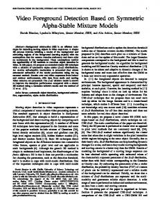
where the lt(u, v) denotes the luminance value in the (u, v) position in a certain t time and the b denotes a threshold value in bin units. A scene change is global if Ldiff exceeds a high percentage of the scene area (Ldiff >= Slimit). The Figure 2 shows five examples where the intersection of the areas below the curves on the figure corresponds a good value space for (b; Slimit). Higher values of the Ldiff are preferred and smaller bins can be caused by the image noise, therefore good sets of values are for example (15; 75), (10; 80) or (20; 70). Any of these options can be used for the Wallflower and the TBMOD videos successfully.
Difference (bins)
100 80 60 40 20 0 50
55
60
65
70
75
80
85
90
95
Scene area (%)
Figure 2. Five examples of illumination changes/sudden reflections from a huge object in various indoor scenes and recorded by multiple cameras. The figure shows the calculated b in the function of Ldiff values between two sequential frames before and after an illumination change. The illumination changes are transient during multiple frames in the records, hence it is a good practice to ignore some frames (e.g. 5 frames in this study) after a change is detected. The Ldiff measure is quite invariant for the image scaling. The L channel scaled to 1/8 of the original size modifies the results of the Ldiff measure less than 1 % and the computation time becomes insignificant at such low resolutions.
3
International Journal of Signal Processing, Image Processing and Pattern Recognition Vol. x, No. x, xxxxx, 2011
2.2. New LBP operator The Local Binary Pattern (LBP) is a grayscale invariant texture primitive statistic, which was introduced in the middle of the nineties. The first version of the operator worked with eight-neighbors of a pixel, using the value of the center pixel as a threshold. The thresholded neighborhood was multiplied with powers of 2 and eventually summing up [10]. Wide variety of the LBP exists in the literature and the version in this paper uses a larger neighborhood than the original. The following formula defines the new operator: 0
1
LBP new ( x , y)=n 1 ( x−2, y−2)∗2 +n2 ( x−2, y )∗2 + 2 3 4 n 1( x+1, y−2)∗2 + n3( x− 2, y)∗2 +n3 ( x+1, y)∗2 + n1 ( x−2, y+1)∗25 +n2 ( x , y+1)∗26+ n 1( x+1, y+1)∗2 7 , i+1 j +1
∑ ∑ g ( u , v) n1 (i , j )= s(
u =i v= j
−C) , 4 g (i , j )+ g (i , j+1) n 2( i , j)=s ( −C) , 2 g (i , j )+g ( i+1, j) n3( i , j)=s ( −C) , 2 s(r )=
(3)
, {10 :: r≥0 r