Aug 1, 2015 - caption = "Housing data linear regression model results"). In order to ..... Dahl DB (2014). xtable: Export Tables to LATEX or HTML. R package ...
JSS
Journal of Statistical Software August 2015, Volume 66, Issue 7.
http://www.jstatsoft.org/
Consistent and Clear Reporting of Results from Diverse Modeling Techniques: The A3 Method Scott Fortmann-Roe University of California, Berkeley
Abstract The measurement and reporting of model error is of basic importance when constructing models. Here, a general method and an R package, A3, are presented to support the assessment and communication of the quality of a model fit along with metrics of variable importance. The presented method is accurate, robust, and adaptable to a wide range of predictive modeling algorithms. The method is described along with case studies and a usage guide. It is shown how the method can be used to obtain more accurate models for prediction and how this may simultaneously lead to altered inferences and conclusions about the impact of potential drivers within a system.
Keywords: goodness of fit, variable importance, model selection.
1. Introduction A range of metrics have been developed to assess model results for prediction or other inferences. These metrics include the classic coefficient of determination and p values, risk functions such as MSE, and newer approaches such as information theoretic techniques like AIC or BIC. Although many methods can be used to assess such error metrics, it can be argued that three basic categories of criteria should be employed to discuss the suitability of these metrics in practice: Accuracy: Does the method accurately report error or goodness of fit? Accessibility: Is the manner in which the results are reported understandable to end-users? Adaptability: Can the method be applied to a variety of different modeling approaches? The importance of accuracy is self-evident. If the method of reporting model quality contains significant biases itself, it may be of little value. The widely reported metric R2 is perhaps
2
The A3 Method for Reporting of Results from Diverse Modeling Techniques
the best example of a commonly used, yet potentially highly inaccurate measure of quality. The key issue with the coefficient of determination is, of course, that it will always increase as more variables are added to the model. The commonly used adjusted R2 measure attempts to account for this issue, but even that may be slightly biased when the model is overfit. Accessibility is of equal importance as accuracy. A metric may objectively be highly accurate, but if practitioners “on the ground” are unable to apply it properly in practice, then it is flawed. An example of a widely discussed measure (Nickerson 2000; Cohen 1994; Loftus 1993; Falk and Greenbaum 1995 and others) that has repeatedly been shown to be inaccessible is the p value. Although the subject of basic statistics courses, p values have been demonstrated to not only be misunderstood by laypeople, but also to be misunderstood by those who absolutely should have a mastery of the topic. In one study of 30 university statistics instructors, 80% made at least one error when answering six basic true/false questions about the interpretation of p values. An example of one such question is, “[Given a p value] you know, if you decide to reject the null hypothesis, the probability that you are making the wrong decision.” (Haller and Krauss 2002). Adaptability is of almost as much importance as accuracy and accessibility. This criterion indicates how flexible the error metric is in regards to being applied to different forms of model construction algorithms. Some metrics – such as AIC or BIC, for instance – require statistical models that generate likelihoods. Many types of models naturally generate likelihoods, but other types of model construction algorithms (such as CART, classification and regression trees; Breiman, Friedman, Olshen, and Stone 1984) may not lend themselves to generating likelihoods. By utilizing a metric that is limited to a certain subspace of model construction algorithms, we limit ourselves in our ability to compare results to other modeling techniques. The A3 method (pronounced A3 ) and the A3 package (Fortmann-Roe 2015) implementation of it for R (R Core Team 2015) targets these three criteria. The method is designed to be accessible, accurate and adaptable (it is from that acronym that the method is named) and the package is available from the Comprehensive R Archive Network (CRAN) at http: //CRAN.R-project.org/package=A3. In terms of accessibility, the method is designed to use familiar concepts. It is based around the R2 metric and p values. Because these metrics are familiar, most practitioners will not have to learn new concepts to understand the A3 output. The A3 method utilizes a derivative of R2 – the added R2 – in order to assess variable importance and the contribution of each feature to the success of the overall model. Unlike likelihood-based approaches – such as AIC-based approaches – or more application specific approaches – such as Gini importance for tree-base methods – this technique is quite general and so can be applied wherever A3 itself may be utilized. The added R2 metric, analogous to semi partial correlation in linear regression, indicates how much a model improves when a given variable is added to the model. This change indicates the practical importance of the added variables which in practice may be more meaningful than statistical significance. The A3 method also provides a slope metric, analogous to the slope in linear regression, to indicate the effect of a variable on the outcome. In summary, the method calculates the following three items for each feature in a data set: Slope: How a change in the feature affects the dependent variable. A distribution of values is calculated for each feature in addition to a single, summarizing average.
Journal of Statistical Software
3
Added R2 : Predictive utility of the feature that is unique from all other features in the model. p value: The chance of seeing the observed level of predictive utility for a feature assuming the null hypothesis that the feature in fact has no predictive utility. Mu˜ noz and van der Laan (2012) introduced a parameter and derived asymptotically linear, semi-parametric estimators of that parameter to quantify the effect of displaced covariates on an outcome. If this parameter were to be normalized by the displacement amount, it would be similar to the slope calculated by the A3 package. In the A3 package, the slope parameter for a feature is estimated by approximating the slope at each data point using simple displacement and then averaging these results. In terms of accuracy, the A3 method uses robust, resampling-based methods for the calculation of p values and R2 metrics. R2 is calculated using cross-validation which correctly accounts for overfitting and does well in matching the true R2 value. The term “R2 ” is defined here simply as the fraction of the squared error explained by a model compared to the null model. This is the definition used in the A3 method’s calculation of R2 and the definition used in the rest of this paper. p values are calculated using a randomization test. Full details about the methods are available in Appendix A. These methods may be computationally intensive for complex models, but they require no parametric assumptions other than independence between observations (a constraint which itself may be violated, see Section 5). The use of these methods make the results reported by the A3 method more robust to user misuse and abuse than do many standard parametric model results (where the parametric assumptions may frequently not be tested for in practice). Last, the A3 method is highly adaptable to different modeling techniques. Technically, the A3 method is defined as a wrapper function that encapsulates an arbitrary predictive modeling algorithm. Thus the method can theoretically be applied to any modeling technique that generates predictions. The same principle is used in the A3 package where the primary package functions can take an arbitrary predictive modeling function. Different modeling methods can be utilized by passing different functions (e.g., lm for linear regression models, glm for logistic regression models, rpart for CART models) to the package’s a3 function. The A3 method can seamlessly encapsulate different techniques and generate a consistent output for them that facilitates the direct comparison of these different methods using the same criteria. It should be noted that the A3 method is focused on inferential statistics and offers little in regards to descriptive statistics or visualizations. There are a wide range of sources addressing and advancing these topics including classics such as Cleveland’s Visualizing Data (Cleveland 1993) and Tukey’s Exploratory Data Analysis (Tukey 1976). R offers a variety of powerful packages to support descriptive analyses. Several R packages such as Hmisc and pastecs provide functions for quickly calculating descriptive statistics (Grosjean and Ibanez 2014; Harrell 2015). Other packages such as data.table or dplyr, in addition to the built-in data.frame, make it straightforward to subset and aggregate data by category (Dowle, Short, Lianoglou, and Srinivasan 2014; Wickham and Fran¸cois 2015). Lastly a number of packages such as the phenomenal ggplot2 make it possible to rapidly create high-quality data visualizations (Wickham 2009). Rather than attempting to improve on these current capabilities in R, the A3 package instead focuses on inferential statistics and prediction.
4
The A3 Method for Reporting of Results from Diverse Modeling Techniques
When the true data-generating process or model is unknown, the A3 method may be used for inference about the significance of features in the data set and for model selection to improve the predictive accuracy of a regression. If the true model were known (or there was strong evidence to justify the adoption of a parametric model), it would of course outperform the semi-parametric models A3 is generally applied to. The following sections of this work will first describe the A3 package in general. Next, two applications of the method are developed for predictive and inferential tasks. Finally, a discussion of using the package to analyze correlated data will be presented followed by general conclusions. One important note should be made at this point. In general, I would make the claim that mathematical models are constructed for three purposes: prediction, inferences other than prediction, and conceptual/narrative applications (e.g., “telling a story about a system”). The A3 package can be applied both to predictive and inferential usage cases. It is based on a predictive framework, but it can also assess the statistical significance of variables within this framework. The key for doing this is to make a small shift in our thinking about inference in order to reframe it in a predictive manner. As an example, take the question “Is there a relationship between X and Y ?” We can rephrase the same question in a predictive framework as “Does knowledge of X help us to predict Y ?” The second question is answered by the A3 package allowing inferences based solely on the predictive accuracy of models.
2. Usage overview The primary function provided by the A3 package is a3 which takes three principle arguments: formula: A regression formula object. data: A data frame containing the data for the regressions. model.fn: A function that generates a regression model that has a corresponding predict method. As example of the usage of the a3 function, we may use R’s built-in lm function with the a3 function to generate the A3 results for a linear regression model of R’s built-in attitude data set. The output is an S3 object with a print method that displays an A3 results table. This table contains four columns: the features in the model, the median slope for each feature (analogous to the coefficient in a linear regression, and directly equivalent to it when used for a linear regression model), the cross-validated R2 for the whole model and the added R2 for each feature (a measure of the practical significance of that feature), and the p values for the model itself and for each feature. R> a3(formula = rating ~ ., data = attitude, model.fn = lm) Average slope -Full model(Intercept) complaints privileges learning
10.78707639 0.61318761 -0.07305014 0.32033212
+ +
CV R^2 p value 47.8 % < 0.01 8.5 % 0.97 10.5 % < 0.01 5.7 % 0.87 7.8 % 0.05
Journal of Statistical Software raises critical advance
0.08173213 0.03838145 -0.21705668 -
6.1 % 8.3 % 3.6 %
5
0.82 0.98 0.59
Please note the p value estimates in this table and the rest of this paper are reported to only two decimals places. This is because the p values were estimated using 100 randomizations. More precise p value estimates can be obtained by increasing the number of random simulations in the calculations of the distribution of R2 values assuming the null hypothesis. For instance, 1,000 randomizations would give an estimate precision of 0.001 but would come at the cost of approximately ten times the computational effort. Refer to Section 4 and Appendix A for more details on the calculation of p values. R comes with numerous predictive modeling algorithms in its core distribution and base packages. An even larger set of modeling techniques are available in the wider ecosystem of user contributed and maintained packages. The a3 method can support most of these techniques (see Appendix B for details). For instance, the e1071 package (Meyer, Dimitriadou, Hornik, Weingessel, and Leisch 2014) provides support vector machine regressions (Cortes and Vapnik 1995) using the function svm. We can use the svm function in place of lm to obtain the A3 results for support vector machines. Please note the use of “+0” in the formula object. This removes the constant term generated in the model matrix which is unnecessary for the svm function. R> library("e1071") R> a3(rating ~ . + 0, attitude, svm) Average slope -Full modelcomplaints privileges learning raises critical advance
0.37018519 0.079660425 0.120305835 0.07477541 -0.138117725 -0.1573689
+ + + +
CV R^2 p value 42.3 % < 0.01 25.3 % < 0.01 3.5 % 0.44 0.9 % 0.14 4.0 % 0.11 11.5 % 0.92 5.4 % 0.06
As another example, we can use the randomForest package (Liaw and Wiener 2002) to generate random forest regressions (Breiman 2001). In order to speed calculation we can set the desired accuracy for the calculation of p values (p.acc) to a coarser value than the default 0.01. Setting p.acc to NULL would disable the calculation of p values completely. R> library("randomForest") R> out.rf out.rf Average slope -Full modelcomplaints privileges learning
CV R^2 p value 43.5 % < 0.05 0.033075 + 26.9 % < 0.05 0 + 2.2 % 1.00 0.0199 + 13.1 % 0.05
6
The A3 Method for Reporting of Results from Diverse Modeling Techniques Average slope -Full modelcomplaints privileges learning raises critical advance
0.033075 0 0.0199 0.036966665 −0.012158335 −0.008216665
CV R2 43.5% +26.9% +2.2% +13.1% +9.7% −0.5% +6.7%
Pr(> R2 ) < 0.05 < 0.05 1.00 0.05 0.25 1.00 0.65
Table 1: LATEX formatted A3 output. raises critical advance
0.036966665 + -0.012158335 -0.008216665 +
9.7 % 0.5 % 6.7 %
0.25 1.00 0.65
Arguments passed to the a3 function are not passed on to the function specified in argument model.fn (in this case randomForest). To pass additional arguments to the function specified in model.fn, you can pass a list of arguments to the argument model.args. For instance, the following code sets the ntree argument of randomForest to 1000. R> a3(rating ~ . + 0, attitude, randomForest, + model.args = list(ntree = 1000), p.acc = 0.05) Average slope -Full modelcomplaints privileges learning raises critical advance
0.042470835 0 0.039183335 0.039104165 -0.00775 -0.02085
+ + + + + +
CV R^2 p value 49.1 % < 0.05 30.1 % < 0.05 4.9 % 0.95 17.7 % < 0.05 9.9 % 0.55 1.0 % 1.00 6.7 % 0.60
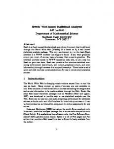
In addition to the general a3 function, we can also use the specialized a3.lm function specifically for linear models which removes the need for the argument model.fn (it is set automatically to glm). Both a3 and a3.lm return an S3 ‘A3’ object. The print method for ‘A3’ objects prints an ASCII results table. You can also use the xtable package (Dahl 2014) to create a nicely formatted output table from this object (see Table 1). R> xtable(out.rf, caption = "\\LaTeX \\, formatted A3 output.", + label = "xtableFormat") Several plotting functions are included in the A3 package to display results. plotPredictions is important in assessing the overall predictive accuracy of the model. For each observation in the data set, it plots the predicted and original values along with an optional line marking ideal results. In Figure 1 we can see that our random forest model for the attitude data appears to tend to overestimate ratings for low values and underestimate them for high ratings. R> plotPredictions(out.rf)
Journal of Statistical Software
7
70 65 60 55
Predicted Value
75
Predicted vs Observed
40
50
60
70
80
Observed Value
Figure 1: A plot of predicted versus observed values for the random forest model of the attitude data. privileges
−0.5
0.5
1.5
2.5
1.0
2.0
learning
0.0
0.0
1.0
2.0
0.0 0.5 1.0 1.5 2.0
complaints
−0.5
0.5
−0.5
critical
0.5
1.5
advance
−0.5
0.5
1.5
0
0
0
1
1
1
2
2
2
3
3
3
4
4
raises
0.0
−0.4
0.0
0.2
−0.4
0.0 0.2 0.4
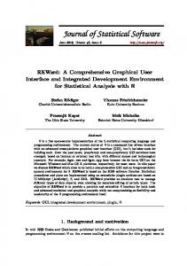
Figure 2: Slope distributions for the random forest model of the attitude data. In the results table, the median of the slopes at each observation are reported. These slopes indicate how the prediction for an observation will change as an observation is displaced (or, put another way, whether a given feature has a positive or negative effect on the outcome
8
The A3 Method for Reporting of Results from Diverse Modeling Techniques
and how strong this effect is). A slope is calculated for each feature at each data point. The slope is approximated by calculating the value of the outcome at a pair of customizable, fixed displacements from each point. For linear regressions, this procedure will result in the same value as the regression coefficients. A fixed displacement is used rather than attempting to estimate the derivative directly at each point as methods such as random forests will often place a step function at data points leading to undefined derivatives at the points themselves. For some models, such as linear regressions, this slope will be constant between observations. However, for other models, such as random forests, the slope may change at each point as the model’s behavior may differ between regions of the feature space. The plotSlopes function may be used to plot the distribution of slopes for each feature (see Figure 2). R> plotSlopes(out.rf) The plot method for ‘A3’ objects may be used to plot both the predictions and slopes at once.
3. Worked applications The most effective way to illustrate the use of the A3 package and its utility is through applied case studies. Two example applications will be used to illustrate the method. The first comes from an attempt to predict housing prices, the second is focused on drawing inferences in an ecological application.
3.1. Housing application This application is based on a data set that includes information on the prices of houses from the Boston area. It originally was developed by Harrison and Rubinfeld (1978) and the digital copy used in this analysis was provided by Frank and Asuncion (2010). The data set is included in the A3 package as housing. The following are some of the key features in the data set (based on the summary of Frank and Asuncion 2010). NOX: Nitrogen oxides pollutant concentration (parts per 10 million). ROOMS: Average number of rooms per dwelling. AGE: Proportion of owner-occupied units built prior to 1940. HIGHWAY: Index of accessibility to radial highways. PUPIL.TEACHER: Pupil-teacher ratio by town. MED.VALUE: Median value of owner-occupied homes in $1,000’s. A typical approach to analyzing this data set, either to build a predictive model or for inferences about the significances of the features, might be to apply a linear regression to the data set (it is important to note that the authors of the cited paper carry out a different form of analysis and this section is simply illustrative of a commonly applied approach). The results of a linear regression are shown in Table 2. Although these specific results are generated by R, the selection of displayed data is very similar to that of other packages. These results allow
Journal of Statistical Software
(Intercept) AGE ROOMS NOX PUPIL.TEACHER HIGHWAY
Estimate 7.7674 −0.0151 7.0056 −13.3142 −1.1165 −0.0249
Std. error 4.9888 0.0138 0.4117 3.9026 0.1480 0.0426
t value 1.56 −1.10 17.02 −3.41 −7.54 −0.58
9 Pr(> |t|) 0.1201 0.2738 0.0000 0.0007 0.0000 0.5593
Table 2: Housing data linear regression model results (R2 = 0.6037, Adjusted R2 = 0.5997). us to clearly see that ROOMS, NOX, and PUPIL.TEACHER are statistically significant variables at the 5% level. However, they do not provide information on the practical importance of these variables in regards to prediction accuracy. R> data("housing", package = "A3") R> reg print.reg(reg, label = "HousingLinear", + caption = "Housing data linear regression model results") In order to attempt to gain an understanding of the practical significance of the different variables, we can use the A3 results. Table 3 contains the A3 results for a linear regression of the housing data. The primary changes in the physical construction of this table is the removal of the standard error and t value columns and the addition of the cross-validated R2 column. This column first reports the R2 for the whole model, and then the added R2 ’s for each feature. The cross-validated R2 is slightly lower, as will generally be the case for overfitting models, than the adjusted R2 . From the added R2 measures reported in the cross-validated R2 column, it can be seen that the ROOMS variable explains 23% more of the squared error when it is added to the model while the NOX variable explains less than 1% of the squared error when it is added to the model. Although both these variables are highly statistically significant (p < 0.01), the A3 output makes it very clear that ROOMS is a much more important predictor of housing prices than NOX. In applications, this information may have great practical importance. R> housing.lm housing.svm R2 ) < 0.01 0.26 0.25 < 0.01 < 0.01 < 0.01 0.96
Table 3: Housing data A3 results for a linear regression model. Average slope -Full modelAGE ROOMS NOX PUPIL.TEACHER HIGHWAY
−0.069444 5.188636 −0.000581 −0.247277 0.042276
CV R2 70.9% +0.9% +34.7% +2.2% +1.6% −0.3%
Pr(> R2 ) < 0.01 0.01 < 0.01 < 0.01 < 0.01 0.16
Table 4: Housing data A3 results for the support vector machine model. Average slope -Full modelAGE ROOMS NOX PUPIL.TEACHER HIGHWAY
−0.0346 4.5326 −1.4777 -0.7140 0.0000
CV R2 74.1% −1.1% +20.3% +6.1% −1.1% −2.2%
Pr(> R2 ) < 0.01 < 0.01 < 0.01 < 0.01 < 0.01 0.02
Table 5: Housing data A3 results for the random forest model. R> housing.rf plotSlopes(housing.rf) From this figure it can be seen that the variable NOX always has a negative effect while a variable such as AGE has differing effects – sometimes negative and sometimes positive – depending on where a specific observation fits.
3.2. Ecology application This case study relates a dryland ecosystem’s multifunctionality (roughly speaking, the magnitude of different services performed by an ecosystem) to a range of environmental variables. It was collected by a large team of researchers and published in the journal Science along with a statistical analysis (Maestre et al. 2012). A copy of the data set is provided by the A3 package in the data variable multifunctionality. The following features are in the data set: ELE: Elevation of the site. LAT and LONG: Location of the site. SLO: Site slope.
12
The A3 Method for Reporting of Results from Diverse Modeling Techniques
(Intercept) SR SLO SAC PCA_C1 PCA_C2 PCA_C3 PCA_C4 LAT LONG ELE
Estimate 1.0081 0.0099 0.0176 −0.0174 −0.0209 −0.0677 0.0348 −0.2663 0.0024 −0.0019 −0.0002
Std. error 0.1747 0.0042 0.0056 0.0020 0.0389 0.0527 0.0355 0.0380 0.0013 0.0005 0.0001
t value 5.77 2.35 3.14 −8.52 −0.54 −1.28 0.98 −7.00 1.80 −3.47 −3.89
Pr(> |t|) 0.0000 0.0197 0.0019 0.0000 0.5918 0.2004 0.3285 0.0000 0.0737 0.0006 0.0001
Table 6: Multifunctionality data linear regression model results (R2 = 0.5645, Adjusted R2 = 0.5441). SAC: Soil sand content. PCA_C1, PCA_C2, PCA_C3, PCA_C4: Principal components of a set of 21 climatic features. SR: Species richness. MUL: Multifunctionality. The original data were analyzed using a multi-model inference approach after Burnham and Anderson (2002). Although the authors also looked at a simultaneous autoregression model, only linear regressions were considered in this multi-model inference and so will be the focus of this reanalysis. The full linear regression explored in the original work is shown in Table 6 with all other linear regressions explored in their work being subsets of this one. From the table, we can see that SR, SLO, SAC, PCA_C4, LONG, and ELE are all statistically significant at the 5% level. R> data("multifunctionality", package = "A3") R> reg print.reg(reg, label = "MFLinear", caption = + "Multifunctionality data linear regression model results") However, as with the housing application, we are again missing information on the importance of each of these variables in regards to the actual predictive accuracy of the model. This information is simply not available in the standard linear regression output table. The A3 method, however, makes it very clear. As shown in Table 7, SAC explains the greatest additional squared error when added to the model, followed by PCA_C4. This basic conclusion agrees with the conclusions of the original researchers as they note, “By this criterion [the sum of Akaike weights across models], the two most important predictors of multifunctionality were annual mean temperature (reflected in ... [PCA_C4]) and the sand content in the soil [SAC].”
Journal of Statistical Software Average slope -Full model(Intercept) SR SLO SAC PCA_C1 PCA_C2 PCA_C3 PCA_C4 LAT LONG ELE
1.00810 0.00989 0.01761 −0.01742 −0.02087 −0.06771 0.03479 -0.26630 0.00235 −0.00187 −0.00025
CV R2 52.6% +7.2% +0.9% +1.8% +16.5% −0.5% +0.1% −0.2% +10.6% +0.2% +2.3% +2.8%
13 Pr(> R2 ) < 0.01 < 0.01 < 0.01 < 0.01 < 0.01 0.92 0.12 0.25 < 0.01 0.06 < 0.01 < 0.01
Table 7: Multifunctionality data A3 Results for a linear regression model. Average slope -Full modelSR SLO SAC PCA_C1 PCA_C2 PCA_C3 PCA_C4 LAT LONG ELE
0.001592 0.002248 −0.004656 0.072615 0.027495 0.015621 -0.090020 0.012747 0.000476 0.000000
CV R2 67.9% +1.2% −1.4% +3.4% +1.5% +0.3% −0.1% +0.7% +0.9% +0.4% +0.4%
Pr(> R2 ) < 0.01 < 0.01 0.87 < 0.01 < 0.01 0.01 0.24 < 0.01 < 0.01 0.04 < 0.01
Table 8: Multifunctionality data A3 results for the random forest model. R> mult.lm mult.rf R> + + + + R> + R> R> +
set.seed(1) createAutoCorrelatedSeries out xtable(out, label = "A3AutoCorCorrect", caption = + "A3 corrected $p$~values accounting for auto-correlation.")
6. Conclusions As a thought experiment, we can use the metaphor of a mountain range to describe the space of all models. Each latitude and longitude in the range represents a different model and the height of the range at that point corresponds to the accuracy of that model given a prediction
Journal of Statistical Software
17
task. Each peak in the range might consist of a single type of model. For instance, one peak might correspond to linear regressions, another peak to support vector machines, yet another peak to a set of mechanistic models, and so on. What is often done in practice when building models for prediction or other inferences is to explore only one peak in this range of mountains. Whether it be just linear regressions or some other technique, researchers and practitioners often only explore a single model family and then make broad conclusions based on the results of this limited analysis. Conclusions drawn from such a narrow exploration of the model space cannot but be viewed with skepticism. In practice, it is almost impossible to say a priori for an unknown data generating process that, for instance, a linear regression model will do the best job of available algorithms in approximating it. It is imperative that practitioners attempt to further explore the model space beyond a single peak – beyond a single model family. The A3 package facilitates this exploration by defining an adaptable algorithm and reporting format that allows the direct comparison of results between different predictive model families. When predictions and statistical measures of significance drawn from models affect policy and scientific decisions, it is of great importance that the best suited modeling techniques available be used. The two worked applications in this paper have demonstrated the use of the A3 package to facilitate the exploration of the model space. In both cases, it was a straightforward process to obtain significantly more predictive models (10%–15% additional explanation of the squared error) compared to the linear regression models simply by exploring one or two additional model families. More importantly, the more predictive models revealed altered conclusions about the significance of the drivers of the systems. Variables that were not statistically significant in the linear regression model became statistically significant in the more predictive random forest models, and vice versa. The ease at which our scientific conclusions can change when we apply more accurate models should be strong motivation to explore a greater part of this infinitely large range of models. The A3 method is just one tool to facilitate this exploration.
Computational details The analyses in this article were conducted using the following software versions R 2.15.2, A3 0.9.2, e1071 1.6-1, pbapply 1.0-5, randomForest 4.6-7, and xtable 1.7-1 When using more recent versions of R and these packages, small differences in results as compared to the replication script may be observed due to the stochastic nature of the A3 method. Despite these small differences, the results remain qualitatively equivalent.
References Breiman L (2001). “Random Forests.” Machine Learning, 45(1), 5–32. Breiman L, Friedman JH, Olshen RA, Stone CJ (1984). Classification and Regression Trees. Wadsworth, California. Burnham KP, Anderson DR (2002). Model Selection and Multimodel Inference: A Practical Information-Theoretic Approach. Springer-Verlag.
18
The A3 Method for Reporting of Results from Diverse Modeling Techniques
Cleveland W (1993). Visualizing Data. Hobart Press, Summit. Cohen J (1994). “The Earth Is Round (p < .05).” American Psychologist, 49(12), 997–1003. Cortes C, Vapnik V (1995). “Support-Vector Networks.” Machine Learning, 20(3), 273–297. Dahl DB (2014). xtable: Export Tables to LATEX or HTML. R package version 1.7-4, URL http://CRAN.R-project.org/package=xtable. Dowle M, Short T, Lianoglou S, Srinivasan A (2014). data.table: Extension of data.frame. R package version 1.9.4; with contributions from R Saporta and E Antonyan, URL http: //CRAN.R-project.org/package=data.table. Falk R, Greenbaum CW (1995). “Significance Tests Die Hard: The Amazing Persistence of a Probabilistic Misconception.” Theory & Psychology, 5(1), 75–98. Fortmann-Roe S (2015). A3: Accurate, Adaptable and Accessible Model Error Metrics. R package version 1.0.0, URL http://CRAN.R-project.org/package=A3. Frank A, Asuncion A (2010). “UCI Machine Learning Repository.” University of California, Irvine, School of Information and Computer Sciences. URL http://archive.ics.uci. edu/ml. Grosjean P, Ibanez F (2014). pastecs: Package for Analysis of Space-Time Ecological Series. R package version 1.3-18, URL http://CRAN.R-project.org/package=pastecs. Haller H, Krauss S (2002). “Misinterpretations of Significance: A Problem Students Share with Their Teachers.” Methods of Psychological Research Online, 7(1), 1–20. Harrell Jr FE (2015). Hmisc: Harrell Miscellaneous. R package version 3.16-0; with contributions from Charles Dupont and many others, URL http://CRAN.R-project.org/ package=Hmisc. Harrison D, Rubinfeld DL (1978). “Hedonic Housing Prices and the Demand for Clean Air.” Journal of Environmental Economics and Management, 5(1), 81–102. Liaw A, Wiener M (2002). “Classification and Regression by randomForest.” R News, 2(3), 18–22. Loftus GR (1993). “A Picture is Worth a Thousand p Values: On the Irrelevance of Hypothesis Testing in the Microcomputer Age.” Behavior Research Methods, 25(2), 250–256. Maestre FT, Quero JL, Gotelli NJ, Escudero A, Ochoa V, Delgado-Baquerizo M, GarciaGomez M, Bowker MA, Soliveres S, Escolar C, Garcia-Palacios P, Berdugo M, Valencia E, Gozalo B, Gallardo A, Aguilera L, Arredondo T, Blones J, Boeken B, Bran D, Conceicao AA, Cabrera O, Chaieb M, Derak M, Eldridge DJ, Espinosa CI, Florentino A, Gaitan J, Gatica MG, Ghiloufi W, Gomez-Gonzalez S, Gutierrez JR, Hernandez RM, Huang X, Huber-Sannwald E, Jankju M, Miriti M, Monerris J, Mau RL, Morici E, Naseri K, Ospina A, Polo V, Prina A, Pucheta E, Ramirez-Collantes DA, Romao R, Tighe M, Torres-Diaz C, Val J, Veiga JP, Wang D, Zaady E (2012). “Plant Species Richness and Ecosystem Multifunctionality in Global Drylands.” Science, 335(6065), 214–218.
Journal of Statistical Software
19
Meyer D, Dimitriadou E, Hornik K, Weingessel A, Leisch F (2014). e1071: Misc Functions of the Department of Statistics (e1071), TU Wien. R package version 1.6-4, URL http: //CRAN.R-project.org/package=e1071. Mu˜ noz ID, van der Laan M (2012). “Population Intervention Causal Effects Based on Stochastic Interventions.” Biometrics, 68(2), 541–549. Nickerson RS (2000). “Null Hypothesis Significance Testing: A Review of an Old and Continuing Controversy.” Psychological Methods, 5(2), 241–301. R Core Team (2015). R: A Language and Environment for Statistical Computing. R Foundation for Statistical Computing, Vienna, Austria. URL http://www.R-project.org/. Stone M (1974). “Cross-Validatory Choice and Assessment of Statistical Predictions.” Journal of the Royal Statistical Society B, 36(2), 111–147. Tukey JW (1976). Exploratory Data Analysis. Addison-Wesley, Massachusetts. Wickham H (2009). ggplot2: Elegant Graphics for Data Analysis. Springer-Verlag, New York. Wickham H, Fran¸cois R (2015). dplyr: A Grammar of Data Manipulation. R package version 0.4.1, URL http://CRAN.R-project.org/package=dplyr.
20
The A3 Method for Reporting of Results from Diverse Modeling Techniques
A. Algorithm details This appendix describes the primary algorithms used by the A3 package. It provides brief narrative descriptions along with algorithmic outlines. For further details, the commented source code in the package itself should be referred to.
A.1. Slopes The A3 package calculates a measure of slope for each feature that is is approximately analogous to the regression coefficient in linear regressions (and in fact it reduces to the regression coefficient when applied to linear regression models). One common way coefficients are described when discussing linear regressions is that they represent how much the dependent variable changes for one unit of change in the independent variable. The slope as reported by the A3 package is calculated in directly this way and is done so for each point in the data set. The reason that this apparently crude measure approximation of slope is used, rather than attempting to actually estimate the derivative right at each point, is that many models generate non-smooth functions (CART, random forests, etc). For instance, in a random forest model, the exact slope at a point will either be 0 (if there is not a branch at that point), or infinite (if there is a branch). Thus the straightforward ±n metric (where n is a user-adjustable value which may vary by feature) is used instead of attempting to precisely estimate the derivative at a point.
function Slopes(Features, Results, n) Data: The data includes Features, a matrix where each column is a feature and each row an observation, and Results, a vector where each element corresponds to a row in the Features matrix. A model construction algorithm FitModel is also assumed with the resulting model having a PredictResult function. Result: A vector of slopes for each feature at each observation. Slopes = []; M odel = F itM odel(F eatures); for F eature ∈ Columns(F eatures) do Slopes[F eature] = []; for Observation ∈ Rows(F eatures) do Lower = Clone(F eatures); Lower[Observation, F eature] = Lower[Observation, F eature] − n; LowerV alue = M odel.P redictResult(Lower); U pper = Clone(F eatures); U pper[Observation, F eature] = U pper[Observation, F eature] + n; U pperV alue = M odel.P redictResult(U pper); Slopes[F eature][Observation] = (U pperV alue − LowerV alue)/2; end end return Slopes end Algorithm 1: The calculation of slope distributions.
Journal of Statistical Software
21
function CrossValidatedR2 (Features, Results) Data: The data includes Features, a matrix where each column is a feature and each row an observation, and Results, a vector where each element corresponds to a row in the Features matrix. A model construction algorithm FitModel is also assumed with the resulting model having a PredictResult function. Result: The cross-validated R2 for the model construction algorithm and data set. This version of the algorithm uses leave-one-out cross-validation. SumSquaredErrorN ull = 0; SumSquaredErrorM odel = 0; for Observation ∈ Rows(F eatures) do SumSquaredErrorN ull = SumSquaredErrorN ull + (M ean(Results[−Observation]) − Results[Observation])2 ; M odel = F itM odel(F eatures[−Observation, AllColumns]); SumSquaredErrorM odel = SumSquaredErrorM odel + (M odel.P redictResult(F eatures[Observation, AllColumns]) − Results[Observation])2 ; end 2 RCrossV alidated = 1 − SumSquaredErrorM odel /SumSquaredErrorN ull ; 2 return RCrossV alidated ; end Algorithm 2: Calculation of cross-validated R2 .
A.2. Cross-validated R2 The calculation of cross-validated R2 is straightforward. Cross-validation is a widely used technique in which a data set is divided into smaller subsets and where the error for each subset is determined using a model developed without that subset (Stone 1974). The A3 package supports k-fold cross-validation. Algorithm 2 details the calculation of the crossvalidated R2 using leave-one-out cross-validation (when the k in k-fold cross-validation is the number of observations). Algorithm 3 details the calculation of the added R2 ’s in the model. These indicate how much the predictive accuracy of the model is increased when a given feature is added to the model. This is analogous to semi-partial correlation in linear regression.
A.3. p values The calculation of p values is done using a randomization test where the accuracy of the added cross-validated R2 for a portion of the data is compared to that for randomly generated data. Assuming the properties of the randomized data are the same as for the real data, the distribution of R2 values obtained using the randomized data represents the distribution of R2 values were the null hypothesis is true. A p value is than estimated by finding the position of the observed R2 values within this distribution. A suitable method for generating the stochastic data must be chosen such that the simulated data has the same properties as the actual data. For independent and identically distributed data, a resampling method is used by default in the A3. For correlated data, more complex techniques must be used. The A3 package comes with a function a3.gen.autocor to help generating stochastic data for
22
The A3 Method for Reporting of Results from Diverse Modeling Techniques
function AddedR2 (Features, Results) Data: The data includes Features, a matrix where each column is a feature and each row an observation, and Results, a vector where each element corresponds to a row in the Features matrix. Result: A vector of added R2 ’s corresponding to each of the features in the model. RF2 ullM odel = CrossV alidatedR2 (F eatures, Results); 2 RAdded = []; for F eature ∈ Columns(F eatures) do 2 RSubmodel = CrossV alidatedR2 (F eatures[AllRows, −F eature], Results); 2 2 RAdded [F eature] = RF2 ullM odel − RSubmodel ; end 2 return RAdded ; end Algorithm 3: Calculation of added R2 ’s. function pValue(Features, Results, Accuracy) Data: The data includes Features, a matrix where each column is a feature and each row an observation, Results, a vector where each element corresponds to a row in the Features matrix, and Accuracy, the desired accuracy for p values. The existence is also assumed of a function GenerateRandomFeatures that creates stochastic noise with the same properties as the Features matrix. Result: The p value for the significance of the entire model. Iterations = Ceiling(1/Accuracy); 2 ROriginal = CrossV alidatedR2 (F eatures, Results); 2 RStochastic = []; for i ∈ [1..Iterations] do DataV ector = GenerateRandomF eatures(F eatures); 2 RStochastic [i] = CrossV alidatedR2 (DataV ector, Results); end 2 2 p = 1 − Quantile(ROriginal , Sort(RStochastic )); return p end Algorithm 4: Calculation of p values.
first-order auto-correlated data such as may sometimes be applicable to temporal data. The basic algorithm is detailed in Algorithm 4. The same technique can also be applied to calculated the significance of individual features.
B. Integration The a3 function, in effect, “wraps” an existing algorithm and generates its statistics based on the output of the method it is wrapping. As such, there is necessarily a level of abstraction when using the A3 method that may make it difficult to fully utilize the unique features of a given modeling technique that could be used if the modeling technique were applied directly.
Journal of Statistical Software
23
The technique it uses to carry out this wrapping works for many existing R model construction functions. However, in some cases the implementation of the target model construction algorithm may make it fail. In these instances, custom code may be required to bridge the A3 package and the target model construction algorithm. The a3 method assumes the following properties of a model function denoted f : f accepts a formula argument that specifies a regression relationship. f accepts a data argument that contains a data frame for the specified formula. f returns a model object for which a predict method has been defined. This predict method’s first argument should be the regression model and the second argument should be new data from which to generate predictions.
Many, built-in R functions conform to these three criteria as do many user contributed packages and functions. However, in cases where a function does not conform to this specification, custom code may be written to allow to use the function with the a3 function. As an example, the following general framework could be used. In it, we create a wrapper for a model with an associated predict function. We then call a3 using the wrapper function. R> + + + + R> + + R>
customFunction.wrapper