22 May 2015 - a locally finite graphs (the adjacency matrix, two discrete Laplacians ... A graph G is locally finite if dG(x) is finite for all x â V. In the sequel, we ...
arXiv:1505.06109v1 [math.SP] 22 May 2015
THE ADJACENCY MATRIX AND THE DISCRETE LAPLACIAN ACTING ON FORMS ´ HATEM BALOUDI, SYLVAIN GOLENIA, AND AREF JERIBI
Abstract. We study the relationship between the adjacency matrix and the discrete Laplacian acting on 1-forms. We also prove that if the adjacency matrix is bounded from below it is not necessarily essentially self-adjoint. We discuss the question of essential self-adjointness and the notion of completeness.
1. Introduction Given a simple graph, the adjacency matrix A is unbounded from above if and only if the degree of the graph is unbounded. It is more complicated to characterize the fact that it is unbounded from below. In [Go] one gives an optimal and necessary. The examples provided in [Go] satisfy : 1) A is not bounded from above, 2) A is bounded from below, 3) A is essentially self-adjoint.
In [Go], one asks the question. Can we have 1 and 2 without having 3? In Corollary 5.3 we answer positively to this question. Moreover, relying on different ideas than in [Go], we provide a large class of graphs satisfying 1 and 2. Our approach is based on establishing a link between the adjacency matrices and the discrete Laplacian ∆1 acting on 1-forms. The article is organized as follows: In Section 2, we present general definitions about graphs. Then we define five different types of discrete operator associated to a locally finite graphs (the adjacency matrix, two discrete Laplacians acting on vertices, two discrete Laplacians acting on edges). The link between these definitions is made in Section 3.2. In Section 4, we start with the question of unboundedness and give a upper bound on the infimum of the essential spectrum. In Section 5.1 we provide a counter example to essential self-adjointness for the Laplacian acting on 1-forms. In Section 5.2 we present the notion of χ-completeness which was introduced in [AnTo] and develop it through optimal examples. Then in Section 5.3 we confront this criterion to other type of approaches. Finally in Section 5.4 we provide a new criterion of essential self-adjointness for the adjacency matrix. Acknowledgment. SG was partially supported by the ANR project GeRaSic (ANR-13-BS01-0007-01) and SQFT (ANR-12-JS01-0008-01). HB enjoyed the hospitality of Bordeaux University when this work started. We would like to thank Michel Bonnefont for useful discussions. 2010 Mathematics Subject Classification. 81Q35, 47B25, 05C63. Key words and phrases. discrete Laplacian, locally finite graphs, self-adjoint extension, adjacency matrix, forms. 1
2
´ HATEM BALOUDI, SYLVAIN GOLENIA, AND AREF JERIBI
2. Graph structures 2.1. Generalities about graphs. We recall some standard definitions of graph theory. A graph is a triple G := (E, V, m), where V is countable set (the vertices), E : V × V → R+ (the edges) is symmetric, and m : V → (0, ∞) is a weight. When m = 1, we simply write G = (E, V). We say that G is simple if m = 1 and E : V × V → {0, 1}. Given x, y ∈ V, we say that x and y are neighbors if E(x, y) > 0. We denote this relationship by x ∼ y and the set of neighbors of x by NG (x). We say there is a loop in x ∈ V if E(x, x) > 0. A graph is connected if for all x, y ∈ V, there exists a path γ joining x and y. Here, γ is a sequence x0 , x1 , ..., xn ∈ V such that x = x0 , y = xn , and xj ∼ xj+1 for all 0 ≤ j ≤ n − 1. In this case, we endow V with the metric ρG defined by (1)
ρG (x, y) := inf{|γ|, γ is a path joining x and y}.
A x−triangle given by (x, y, z, x) is different form the one given by (x, z, y, x). A graph G is locally finite if dG (x) is finite for all x ∈ V. In the sequel, we assume that: All graphs are locally finite, connected with no loops. A graph G = (E, V, m) is bi-partite if there are V1 and V2 such that V1 ∩ V2 = ∅, V1 ∪ V2 = V, and such that E(x, y) = 0 for all (x, y) ∈ V12 ∪ V22 . Definition 2.1. Given a graph G = (E, V, m), we define the line graph of G the e V) e where V e is the set of edges of G and graph Ge := (E, p � � pE(x , y )E(x, y) E(x0 , y0 )E(x, y) 0 0 1x=x0 + 1y=y0 , Ee (x0 , y0 ), (x, y) = m(x) m(y)
if (x0 , y0 ) 6= (x, y) and 0 otherwise. The choice of the weight E˜ seems a bit arbitrary but is motivated by Proposition 3.1. We stress that m ˜ = 1. Others choices can be made, e.g., [EvLa]. We refer to [Ha][Chapter 8] for a presentation of this class in the setting of simple graphs.
A bipartite graph G
The line-graph of G
THE ADJACENCY MATRIX AND THE DISCRETE LAPLACIAN ACTING ON FORMS
A graph K1,8
3
g K 1,8 is the complete graph K8
As we see on this example, the line-graph is obtained by gluing together some complete graphs. This is not true in general. The classification of the line-graphs of a finite graph is well-known, see [Ha][Theorem 8.4]. We present the relationship between bipartite graphs and line graphs. We recall that Cn denotes the n-cycle graph, i.e., V := Z/nZ, where E(x, y) = 1 if and only if |x − y| = 1. Proposition 2.2. Let G = (E, V) be a bipartite graph. Then the two following assertions are equivalent: e 1) G ≃ G, 2) G ∈ {Z, N, C2n : n ∈ N}.
e Then Ge not contain Proof. It clear that (2) ⇒ (1). Now, suppose that G ≃ G. e So, x−triangles. If dG (x) ≥ 3, for all x ∈ V, then there exist a x−triangle of G. dG (x) ≤ 2 ∀x ∈ V. This proof is complete. � 2.2. The adjacency matrix. Set G = (E, V, m) a weighted graph. We define the set of 0−cochains C(V) := {f : V → C}. We denote by C c (V) the 0-cochains with finite support in V. We associate a Hilbert space to V. ( ) X 2 2 2 ℓ (V) := f ∈ C(V) such that kf k := m(x)|f (x)| < ∞ . x∈V
The associated scalar product is given by X hf, gi := m(x)f (x)g(x), for f, g ∈ ℓ2 (V). x∈V
We define the adjacency matrix :
AG (f )(x) := c
1 X E(x, y)f (y) m(x) y∈V
for f ∈ C (V). It is symmetric and thus closable. We denote its closure by the same symbol. We denote the degree by 1 X degG (x) := E(x, y). m(x) y∈V
When m = 1, we have that AG is unbounded if and only it is unbounded from above and if and only if the degree is unbounded. The fact that AG is unbounded from
´ HATEM BALOUDI, SYLVAIN GOLENIA, AND AREF JERIBI
4
below or not is a delicate question, see [Go]. We refer to [GoSc] for the description of some self-adjoint extensions. 3. The laplacians acting on edges 3.1. The symmetric and anti-symmetric spaces. In the previous section we defined a Hilbert structure on the set of vertices. We can endow two different Hilbert structures on the set of edges. Both have their own interest. Given a weighted graph G = (E, V, m), the set of 1−cochains (or 1-forms) is given by: Canti (E) := {f : V × V → C, f (x, y) = −f (y, x) for all x, y ∈ V},
where anti stands for anti-symmetric. This corresponds to fermionic statistics. Concerning bosonic statistics, we define: Csym (E) := {f : V × V → C, f (x, y) = f (y, x) for all x, y ∈ V}.
c c The sets of functions with finite support are denoted by Canti (E) and Csym (E), respectively. We turn to the Hilbert structures. X 1 ℓ2anti (E) := f ∈ Canti (E) such that kf k2 := E(x, y)|f (x, y)|2 < ∞ 2 x,y∈V
and
X 1 ℓ2sym (E) := f ∈ Csym (E) such that kf k2 := E(x, y)|f (x, y)|2 < ∞ . 2 x,y∈V
The associated scalar product is given by 1 X E(x, y)f (x, y)g(x, y), hf, gi := 2 x,y∈V
ℓ2anti (E)
when f and g are both in or in ℓ2sym (E). We start by defining operator in the anti-symmetric case. The difference operator is defined as c d := danti : C c (V) −→ Canti (E), d(f )(x, y) := f (y) − f (x).
The coboundary operator is the formal adjoint of d. We set: 1 X c d∗ := d∗anti : Canti (E) −→ C c (V), d∗ (f )(x) := E(y, x)f (y, x). m(x) y∈V
We denote by the same symbols their closures. The Gauß-Bonnet operator is dec fined on C c (V) ⊕ Canti (E) by � � 0 d∗ ∗ ∼ . D := d + d = d 0
This operator is motivated by geometry, see [AnTo]. It is also a Dirac-like operator. The associated Laplacian is defined as ∆ := D2 = ∆0 ⊕ ∆1 where ∆0 is the discrete Laplacian acting on 0−forms given by 1 X E(x, y)(f (x) − f (y)), (2) ∆0 (f )(x) := (d∗ d)(f )(x) = m(x) y
THE ADJACENCY MATRIX AND THE DISCRETE LAPLACIAN ACTING ON FORMS
5
with f ∈ C c (V), and where the discrete Laplacian acting on 1−forms is given by (3)
∆1 (f )(x, y) := (dd∗ )(f )(x, y) 1 X 1 X = E(x, z)f (x, z) + E(z, y)f (z, y), m(x) m(y) z∈V
z∈V
c with f ∈ Canti (E). Both operator are symmetric and thus closable. We denote the closure by ∆0 (resp. ∆1 ), its domain by D(∆0 ) (resp. D(∆1 )), and its adjoint by ∆∗0 (resp. ∆∗1 ). In [Wo], one proves that ∆0 is essentially self-adjoint on C c (V) when the graph is simple. The literature on the subject is large and refer to [Go2] for historical c purposes. In [AnTo], they prove that D is essentially self-adjoint on C c (V)⊕Canti (E) c c if and only if ∆0 ⊕ ∆1 is essentially self-adjoint on C (V) ⊕ Canti (E). Moreover they provide a criterion based on the completeness of a metric. In Section 5.1 we provide a counter example to essential self-adjointness for the Laplacian acting of 1-forms. Then in Section 5.2 we discuss the notion of χ-completeness that was introduced in [AnTo]. This notion is related to the one of intrinsic metric, e.g., [HKMW] and references therein. We turn to the symmetric choice. We set : c dsym : C c (V) −→ Csym (E), dsym (f )(x, y) := f (y) + f (x).
It is interesting to note that dsym is in fact the incidence matrix of G. Indeed � 1, if x0 ∈ {x, y}, dsym (δx0 )(x, y) = 0, otherwise. The formal adjoint of the incidence matrix is given by: 1 X c E(y, x)f (y, x). d∗sym : Csym (E) −→ C c (V), d∗sym (f )(x) := m(x) y∈V
A direct computation gives that :
∆0,sym f (x) := (d∗sym dsym )f (x) = for all f ∈ C c (V) and (4)
1 X E(x, y)(f (x) + f (y)), m(x) y
∆1,sym f (x, y) := (dsym d∗sym )f (x, y) 1 X 1 X E(x, z)f (x, z) + E(z, y)f (z, y), = m(x) m(y) z∈V
z∈V
c Csym (E).
for all f ∈ We denote by the same symbol the closure of these operators. We turn to this central observation. Proposition 3.1. Set G = (E, V, m). The operator ∆1,sym is unitarily equivalent to AG˜ + V (·, ·),
where
V (x, y) := E(x, y)
�
1 1 + m(x) m(y)
and G˜ denotes the line-graph of G, see Definition 2.1.
�
6
´ HATEM BALOUDI, SYLVAIN GOLENIA, AND AREF JERIBI
˜ is not It is important to note that ℓ2sym (E) is a weighted space, whereas ℓ2 (V) one. This proposition is part of the folklore in the case of finite and unweighted graphs. ˜ 1) as being the unitary transformation given by Proof. We set U : ℓ2sym (E) → ℓ2 (V, p U f (x, y) := E(x, y)f (x, y). We have (U ∆1,sym U −1 )f (x, y) = ! p p X E(x, y)E(x, z) E(x, y)E(z, y) f (x, z) + f (z, y) , m(x) m(y) z∈V
e Remembering the definition of the weights for a line-graph, we for all f ∈ C c (V). obtain the result. � Corollary 3.2. Let G = (E, V, m) be a weighted graph. If � � 1 1 0, there is a connected simple graph G such that Cloc (G) ∈ (0, ε), AG is essentially self-adjoint on C c (V) and is bounded from below. The line-graph do not lead to the optimality that is obtained in third point. Indeed, by repeating the proof of [Go, Proposition 3.2] we obtain that given G = (E, V) be a locally finite simple bipartite graph, then sub ˜ Cloc (G) >
1 . 10
THE ADJACENCY MATRIX AND THE DISCRETE LAPLACIAN ACTING ON FORMS
7
3.2. Breaking symmetry. We have that (3) and (4) have the same expression. However they do not act on the same spaces. When G is bi-partite, we shall prove that the two operators are unitarily equivalent. We now fix an orientation of a graph G = (E, V, m). For each edge there are two possible choices. For x, y ∈ V such that E(x, y) 6= 0, we write x → y or y → x, following the choice of the orientation. Let U : ℓ2anti (E) −→ ℓ2sym (E) be the unitary map given by � 1, if x → y, (U f )(x, y) = sign(x, y)f (x, y), where sign(x, y) := −1, if y → x.
Note that (U −1 f )(x, y) = sign(x, y)f (x, y). Therefore, for x0 , y0 ∈ V and f ∈ ℓ2sym (E) we have � 1 X E(x, y0 )sign(x, y0 )f (x, y0 ) U ∆1 U −1 f (x0 , y0 ) = sign(x0 , y0 ) m(y0 ) x∈V � 1 X (5) + E(x0 , y)sign(x0 , y)f (x0 , y) . m(x0 ) y∈V
In order to take advantage of this transformation, one has to choose the orientation in a good way. We have :
Proposition 3.4. Assume that G = (E, V, m) is a bi-partite weighted space, then ∆1 and ∆1,sym are unitarily equivalent. In particular, if we also have that G is simple, ∆1 is unitarily equivalent to AG˜ + 2id. Proof. We consider the bi-partite decomposition {V1 , V2 } of the graph G. For x ∈ V1 and y ∈ V2 , we set x → y. From (5), we see that all the products of the signs are being 1. This gives the first part. For the rest, apply Proposition 3.1. � Since the line-graph of Z is itself and it is also bi-partite, we can make a different choice of orientation. Example 3.5. We consider on Z the orientation n → n + 1, for all n ∈ Z. ˜ ≃ Z. Moreover, we have: Note that Z
(U ∆1 U −1 )f (n, n + 1) = 2f (n, n + 1) − AGef (n, n + 1).
Therefore, ∆1 and 2I − AGe are unitarily equivalent.
4. On the spectral properties of the Laplacian acting on forms We start with the question of unboundedness. Proposition 4.1. Let G = (E, V, m) be a weighted graph. Then ∆1 is bounded if and only if ∆1,sym is bounded if and only if ∆0 is bounded if and only if sup degG (x) < ∞.
x∈V
Proof. The last equivalence is well-known, e.g., [KL2]. On one side we have c
0 ≤ hf, ∆0 f i ≤ hf, 2 degG (·)f i,
for all f ∈ C (V) and on the other side hδx , ∆0 δx i = degG (x). The same statements hold true for ∆0,sym .
´ HATEM BALOUDI, SYLVAIN GOLENIA, AND AREF JERIBI
8
We turn to ∆1 . We denote by F the Friedrichs extension. ∗ ∆1 is bounded ⇔ ∆F 1 is bounded ⇔ d is bounded
⇔ d is bounded ⇔ ∆0 is bounded.
1/2 The second equivalence comes from the fact that k(∆F f k = kd∗ f k, for all 1 ) c f ∈ Canti (E) and by construction of the Friedrichs extension (e.g., [ReSi]). The last one is of the same type. The equivalence with ∆1,sym is similar. � Using the Persson’s Lemma we give the following result:
Proposition 4.2. Let G = (E, V, m) be an infinite and ∆F 1 be a Friedrichs extension of ∆1 . Then � � 1 1 F E(x, y) + inf σ(∆1 ) ≤ inf x,y∈V,x∼y m(x) m(y) and inf σess (∆F 1 ) ≤
inf
infc
K⊂E,Kfinite (x,y)∈K ,x∼y
�
1 1 + m(x) m(y)
�
E(x, y).
In particular, ∆F 1 is not with compact resolvent when G is simple and infinite. The last statement really differs from the situation case of ∆0 . Indeed, in the 1/2 case � sparse graph (a planar graph for instance), one has that D(∆0 ) = � of a simple 1/2 D degG (·) , see [BGK] and also [Go2]. In particular we have that ∆0 is with compact resolvent if and only if lim|x|→∞ degG (x) = ∞.
Proof. Let x0 , y0 ∈ V such that E(x0 , y0 ) 6= 0. Then, * + � � 1 δx0 ,y0 − δy0 ,x0 F � δx0 ,y0 − δy0 ,x0 � 1 p p + E(x0 , y0 ). = , ∆1 m(x0 ) m(y0 ) E(x0 , y0 ) E(x0 , y0 )
Recalling (6)
δ
x0 ,y0 − δy0 ,x0
p
= 1. E(x0 , y0 )
and the Persson’s Lemma, e.g., [KL2][Proposition 18], the result follows.
�
Remark 4.3. The same result holds true for the operator ∆1,sym by changing the − into + in (6). 5. Essential self-adjointness From now on, we concentrate on the analysis of ∆1 . The results for ∆1,sym are the same and the proofs need only minor changes. 5.1. A counter example. First it is important to notice that unlike ∆0 , ∆1 , define as the closure of (3), is not necessarily self-adjoint on simple graphs. Let G = (E, V) be radial simple tree. We denote the origin by ν and the spheres by Sn := {x ∈ V, ρG (ν, x) = n}. Let off(n) := |Sn+1 |/|Sn | be the offspring of the n-th generation.
THE ADJACENCY MATRIX AND THE DISCRETE LAPLACIAN ACTING ON FORMS
9
Theorem 5.1. Let G = (E, V) be a radial simple tree. Suppose that n 7→
(7)
off 2 (n) ∈ ℓ1 (N). off(n + 1)
c Then, ∆1 does not essentially self-adjoint on Canti (E) and the deficiency indices are infinite.
Proof. Set f ∈ ℓ2anti (E) \ {0} such that f ∈ ker(∆∗1 + i) and such that f is constant on Sn × Sn+1 . We denote the constant value by Cn . So, we have the following equation (off(n) + 1 + i)Cn − Cn+1 off(n + 1) − Cn−1 = 0. Therefore, n+1 Y
f |Sn+1 ×Sn+2 2 = |Cn+1 |2 off(i) i=0
≤2
=2 Since
n+1 n+1 Y 1 |off(n) + 1 − i|2 Y 2 off(i)|C | + 2 off(i)|Cn−1 |2 . n 2 2 off (n + 1) i=0 off (n + 1) i=0
|off(n) + 1 − i|2 off(n) kf |Sn×Sn+1 k2 + 2 kf |Sn−1 ×Sn k2 . off(n + 1) off(n + 1)
off 2 (n) tends to 0 as n goes to infinity, we get by induction: off(n + 1) C := sup kf |Sn ×Sn+1 k2 < ∞. n∈N
Then, we have 2
kf |Sn+1 ×Sn+2 k ≤ 2C
�
off(n) |off(n) + 1 − i|2 + off(n + 1) off(n + 1)
�
.
By (7), we conclude that f ∈ ℓ2 (E) and that dim ker(∆∗1 + i) ≥ 1. Using [ReSi, Theorem X.36] we derive that ∆1 is not essentially self-adjoint. Finally, since the deficiency indices are stable under bounded perturbation, by cutting off the graph large enough, we reproduce the same proof with an arbitrary large number of identical and disjoint trees, we see that dim ker(∆∗1 + i) = ∞. � Remark 5.2. For the adjacency matrix, we are able to construct an example of simple graph where the deficiency indices are equal to 1, see [GoSc2]. The case of ∆1 is more complicated and we were not able to find an example where the deficiency indices are finite. We leave this question open. We can answer a problem which was left open in [GoSc]. Corollary 5.3. There exists a locally finite simple graph G = (E, V) such that AG is bounded from below by −2 and such that AG is not essentially self-adjoint on C c (V). Proof. Combine Theorem 5.1 with Proposition 3.4.
�
´ HATEM BALOUDI, SYLVAIN GOLENIA, AND AREF JERIBI
10
5.2. Completeness. We first recall a criterion obtained in [AnTo]. They introduce the following definition (see references therein for historical purposes). Definition 5.4. The graph G = (E, V, m) is χ−complete if there exists a increasing sequence of finite set (On )n such that V = ∪n On and there exist related functions χn satisfying the following three conditions: 1) χn ∈ C c (V), 0 ≤ χn ≤ 1, 2) χn (x) = 1 if x ∈ On , 3) ∃C > 0, ∀n ∈ N, x ∈ V, such that 1 X E(x, y)|χn (x) − χn (y)|2 ≤ C. m(x) y The result of [AnTo], can be reformulate as follows: Theorem 5.5. Take G = (E, V, m) to be χ−complete. Then ∆1 is essentially c self-adjoint on Canti (E). Remark 5.6. The converse is an open problem. The aim of the next sections is to tackle it. 5.2.1. A sharp example. Theorem 5.5 is abstract and may be difficult to check in concrete settings. In [AnTo], they provide only one example. Moreover, they do not give a concrete way to prove that a graph is not χ-complete. To start-off we provide a sharp example. Proposition 5.7. Let G = (E, V) be a locally finite simple tree, endowed with an origin such that off(n) := off(x) for all x ∈ Sn . Then the graph G is χ−complete is and only if ∞ X 1 p = ∞. off(n) n=1
Example 5.8. Set α > 0. Let G = (E, V) be a locally finite simple tree, endowed with an origin such that off(x) = ⌊nα ⌋ for all x ∈ Sn . Then the graph G is χ−complete is and only if α ≤ 2. Proof. Suppose that the series converges and that G is χ−complete. Let (χn )n∈N be as in the definition. Using 3), we get: √ C |χn (m) − χn (m + 1)| ≤ p . off(m)
Moreover, by convergence of the series, there is N ∈ N such that ∞ X 1 1 p < √ . α ⌊n ⌋ 2 C k=N
Then, by 2), there is n0 ∈ N such that χn0 (x) = 1 for all |x| ≤ N . Since χn0 is with finite support, there is M ∈ N such that χn0 (x) = 0 for all |x| ≥ N + M . Therefore, 1 = |χn0 (N ) − χn0 (N + M )|
≤ |χn0 (N ) − χn0 (N + 1)| + . . . + |χn0 (N + M − 1) − χn0 (N + M )| ≤
X √ N +M−1 1 1 p < . C α 2 ⌊n ⌋ n=N
THE ADJACENCY MATRIX AND THE DISCRETE LAPLACIAN ACTING ON FORMS
11
Contradiction. Therefore if the series converges, then G is not χ−complete. Suppose now that the series diverges. Set 1, if |x| ≤ n, |x|−1 X 1 χn (x) := , if |x| > n. p max 0, 1 − off(k) k=n
Since the series diverges, χn is with compact support and satisfies the definition of χ-completeness. � 5.2.2. 1-dimensional decomposition. We now strengthen the previous example and follow ideas of [BG]. Definition 5.9. A 1-dimensional decomposition of the graph G := (V, E) is a family of finite sets (Sn )n≥0 which forms a partition of V, that is V = ⊔n≥0 Sn , and such that for all x ∈ Sn , y ∈ Sm , E(x, y) > 0 =⇒ |n − m| ≤ 1.
Given such a 1-dimensional decomposition, we write |x| := n if x ∈ Sn . We also write BN := ∪0≤i≤N Si . We stress that S0 is not asked to be a single point. Example 5.10. Typical examples of such a 1-dimensional decomposition are given by level sets of the graph distance function to a finite set S0 that is (8)
Sn := {x ∈ V, ρG (x, S0 ) = n},
where the graph distance function ρG is defined by (1). Note that for a general 1-dimensional decomposition, one has solely ρG (x, S0 ) ≥ n, for x ∈ Sn . We define the inner boundary of Sn by Sn− := {x ∈ Sn , ∃y ∈ Sn−1 , E(x, y) > 0}
and the outer boundary by
Sn+ := {x ∈ Sn , ∃y ∈ Sn+1 , E(x, y) > 0}.
We now divide the degree with respect to the 1-dimensional decomposition. Given x ∈ Sn , we set X 1 X 1 E(x, y), deg0 (x) := E(x, y), deg± (x) := m(x) m(x) y∈Sn±1
y∈Sn
with the convention that S−1 = ∅. Note that deg = deg+ + deg− + deg0 is independent of the choice of a 1-dimensional decomposition. We now give a criterion of essential self-adjointness. Theorem 5.11. Let G = (E, V, m) be a weighted graph and (Sn )n≥0 be a 1dimensional decomposition. Assume that ∞ X 1 q = ∞, + an + a− n=1 n+1 ± deg (x). where a± Then G is χ-complete and in particular, ∆1 is n := supx∈Sn ± c essentially self-adjoint on Canti (E).
´ HATEM BALOUDI, SYLVAIN GOLENIA, AND AREF JERIBI
12
S5 S2 S1
S4 S3
S6
S0
Figure 1. An antitree with spheres S0 , . . . , S6 of sizes 1, 7, 13, 5, 9, 20, 3. Proof. It is enough to check the hypothesis of Theorem 5.5. We set 1, if |x| ≤ n, |x|−1 X 1 χn (x) := , if |x| > n. q max 0, 1 − + − a +a k=n k
k+1
Since the series diverges, χn is with compact support. Note that χn is constant on Sn . If x ∈ Sm with m > n, we have : X 1 1 E(x, y)|χn (x) − χn (y)|2 ≤ deg+ (x) + . m(x) am + a− m+1 y∈Sm+1
1 X E(x, y)|χn (x) − χn (y)|2 = 0 m(x) y∈Sm
1 m(x)
X
y∈Sm−1
E(x, y)|χn (x) − χn (y)|2 ≤ deg− (x)
It satisfies the definition of χ-completeness.
1 −. a+ m−1 + am �
5.2.3. Application to the class of antitrees. We focus on antitrees, see also [Wo2] and [BK]. The sphere of radius n ∈ N around a vertex v ∈ V is the set Sn (v) := {w ∈ V, ρG (v, w) = n}. A graph is an antitree, if there exists a vertex v ∈ V such that for all other vertices w ∈ V \ {v} NG (w) = Sn−1 (v) ∪ Sn+1 (v),
where n = ρG (v, w) ≥ 1. See Figure 1 for an example. The distinguished vertex v is the root of the antitree. Antitrees are bipartite and enjoy radial symmetry. Proposition 5.12. Let G : (E, V) be a simple antitree whose root is v. Set sn := ♯Sn (v). Assume that X 1 =∞ √ sn + sn+1 n∈N
c then G is χ-complete and in particular, ∆1 is essentially self-adjoint on Canti (E).
Proof. Use Theorem 5.11 with Sn := Sn (v).
�
THE ADJACENCY MATRIX AND THE DISCRETE LAPLACIAN ACTING ON FORMS
13
5.3. Other approaches. We present some techniques that ensure essential selfadjointness. Theorem 5.13. Let G = (E, V, m) be a locally finite graph. Set � X� 1 1 E(x, z) + E(z, y) . M(x, y) := 1 + m(x) m(y) z∈V
Suppose that
sup
X
x,y∈V z∈V
1 E(x, z)|M(x, y) − M(x, z)|2 < ∞. m(x)
c Then ∆1 is essentially self-adjoint on Canti (E). c Proof. Take f ∈ Canti (E). We have
k∆1 f k2 ≤
X
(x,y)∈V 2
=2
E(x, y)
X
(x,y)∈V 2
E(x, y)
2 1 X E(x, z)f (x, z) m2 (x) z∈V
1 m2 (x)
2 1 X E(z, y)f (z, y) + 2 m (y) z∈V X 2 E(x, z)f (x, z)
!
z∈V
�� X � 1 �X E(x, t) E(x, z)|f (x, z)|2 E(x, y) 2 ≤2 m (x) t∈V z∈V (x,y)∈V 2 2 1 �X � X E(x, z) f (x, y) ≤ 2kM(·, ·)f k2 . =2 E(x, y) m(x) 2 X
z∈V
(x,y)∈V
Moreover, noting that M c(x, y) = M c(y, x) and that f (x, y) = −f (y, x) we get: 2|hf, [∆1 , M(·, ·)]f i| ≤ kf k2 + �X X E(x, y)
�2 1 E(x, z) M(x, z) − M(x, y) f (x, z) m(x) z∈V (x,y)∈V 2 � X 1 1 �X ≤ kM(·, ·) 2 f k2 + E(x, y) E(x, t) × m(x) t∈V (x,y)∈V 2 �X 2 2 � 1 M(x, z) − M(x, y) f (x, z) E(x, z) m(x) z∈V X 1 X 1 E(x, y) E(x, t) = kM(·, ·) 2 f k2 + m(x) 2 t∈V
(x,y)∈V
X
2 2 1 M(x, y) − M(x, z) f (x, y) E(x, z) m(x) z∈V | {z } ≤C
1
≤ (1 + 2C)kM(·, ·) 2 f k2 .
Applying [ReSi, Theorem X.37], the result follows.
�
14
´ HATEM BALOUDI, SYLVAIN GOLENIA, AND AREF JERIBI
Example 5.14. Take G = (E, V) to be a simple radial tree such that sup |off(n) − off(n + 2)| < ∞,
n∈N
c then ∆1 is essentially self-adjoint on Canti (E).
This example can be reached by Theorem 5.5, however for weighted graphs the hypotheses do not seem to fully overlap from one side or from the other. We now give a more powerful way to check that ∆1 is essentially self-adjoint. It seems that this approach is new in the setting of graphs. Theorem 5.15. Let G = (E, V, m) be a weighted graph. Fix x0 ∈ V and set Bn := {x ∈ V, ρG (x0 , x) ≤ n}. If −1/2n ∞ Y X (9) =∞ sup (degG (x)) n=1
i≤n x∈Bi
c then ∆1 is essentially self-adjoint on Canti (E).
Proof. Since ∆1 is non-negative, by [MaMc] or [Nu], it is enough to prove that for c all f ∈ Canti (E): ∞ X k∆n1 f k−1/2n = ∞. n=0
Set f ∈ There is n0 such that supp f ⊂ Bn2 0 , where Bn2 0 := Bn0 × Bn0 . Note that supp (∆1 )n f ⊂ Bn2 0 +n . Therefore c Canti (E).
k(∆1 )n+1 f k ≤ k1Bn2 ≤
0 +n+1
sup x∈Bn0 +n+1
∆1 1Bn2
0 +n+1
k · k(∆1 )n f k
degG (x) · k(∆1 )n f k
c since, for all g ∈ Canti (E) and k ∈ N, we have: 2 X 1 X E(x, y)1Bk2 (x, y)g(x, y) 0 ≤ h1Bk2 g, ∆1 1Bk2 gi = m(x) y x �X X 1 �X ≤ E(x, y) E(x, z)|1Bk2 (x, z)g(x, z)|2 m(x) x y z
≤ sup deg(x) · k1Bk2 gk2 . x∈Bk
This concludes the proof.
�
Remark 5.16. The example of Proposition 5.7 is also covered by Theorem 5.15. Remark 5.17. A computation shows that the condition (9) is equivalent to ∞ X
n=1
p
1 = ∞, supx∈Bn (degG (x))
when supx∈Bn (degG (x)) is equivalent to nα lnβ (n), as n goes to infinity.
THE ADJACENCY MATRIX AND THE DISCRETE LAPLACIAN ACTING ON FORMS
15
5.4. The case of the Adjacency matrix. We take the opportunity to apply this technique for the adjacency matrix. This improves the results obtained in [GoSc]. Theorem 5.18. Let G = (E, V, m) be a weighted graph. Fix x0 ∈ V and set Bn := {x ∈ V, ρG (x0 , x) ≤ n}. If −1/n ∞ Y X (10) =∞ sup (degG (x)) n=1
i≤n x∈Bi
then AG is essentially self-adjoint on C c (V).
Proof. Since AG is not necessary non-negative, by [MaMc] or [Nu], it is enough to prove that for all f ∈ C c (V) ∞ X
n=0
kAnG f k−1/n = ∞.
Set f ∈ C c (V). There is n0 such that supp f ⊂ Bn0 . Note that supp AnG f ⊂ Bn0 +n . Therefore f k ≤ k1Bn0 +n+1 AG 1Bn0 +n+1 k · kAnG f k kAn+1 G ≤
sup
x∈Bn0 +n+1
degG (x) · kAnG f k
since, for all g ∈ C c (V), we have |hg, AG gi| ≤ hg, degG (·)gi.
�
Corollary 5.19. Let G = (E, V) be a radial simple tree, endowed with an origin such that off(n) := off(x) for all x ∈ Sn . Assume that ∞ X
1 = ∞. off(n) n=1 Then AG is essentially self-adjoint.
Remark 5.20. Note that the condition (10) is not optimal for the question of selfadjointness in the case of a radial simple tree, see [GoSc][Proposition 1.2] but is optimal in the case of anti-trees, see [GoSc2]. To finish denote by G˜ the line graph of a bipartite graph G. Then, thanks to Proposition 3.1, all the criteria of Sections 5.2 and 5.3 implies that AG˜ is essentially ˜ self-adjoint on C c (V). References [AnTo] [BG] [BGK] [BK] [EvLa] [Go]
C. Ann´ e and N. Torki-Hamza: The Gauss-Bonnet operator of an infinite graph, Anal. Math. Phys. (2014). M. Bonnefont and S. Gol´ enia: Essential spectrum and Weyl asymptotics for discrete Laplacians, preprint arXiv:1406.5391. M. Bonnefont, S. Gol´ enia, and M. Keller: Eigenvalue asymptotics for Schr¨ odinger operators on sparse graphs, to appear in Annales de l’institut Fourier. J. Breuer and M. Keller: Spectral Analysis of Certain Spherically Homogeneous Graphs, Operators and Matrices 4, 825-847 (2013) T.S. Evans and R. Lambiotte: Line graphs, link partitions and overlapping communities, Physical Review E 80: 016105 (2009). S. Gol´ enia: Unboundedness of adjacency matrices of locally finite graphs, Lett. Math. Phys. 93, 127–140 (2010).
16
´ HATEM BALOUDI, SYLVAIN GOLENIA, AND AREF JERIBI
[Go2]
S. Gol´ enia: Hardy inequality and asymptotic eigenvalue distribution for discrete Laplacians, J. Func. Anal. 266, 2662–2688 (2014). [GoSc] S. Gol´ enia and C. Schumacher: The problem of deficiency indices for discrete Schr¨ odinger operators on locally finite graphs, J. Math. Phys. 52, 063512, 17 pp. (2011). [GoSc2] S. Gol´ enia and C. Schumacher: Comment on “The problem of deficiency indices for discrete Schr¨ odinger operators on locally finite graphs” [J. Math. Phys. 52, 063512 (2011)], J. Math. Phys. 54, no. 6, 064101, 4 pp. (2013). [Ha] F. Harary: Graph theory, Addison-Wesley Publishing Co., Reading, Mass.-Menlo Park, Calif.-London ix+274 pp. (1969). [HKMW] X. Huang, M. Keller, J. Masamune, and R.K. Wojciechowski: A note on self-adjoint extensions of the Laplacian on weighted graphs, J. Func. Anal. 265, no. 8, (2013). [KL2] M. Keller and D. Lenz: Unbounded Laplacians on graphs: basic spectral properties and the heat equation, Math. Model. Nat. Phenom. 5, no. 4, 198–224 (2010). [MaMc] D. Masson and W.K. McClary: Classes of C ∞ vectors and essential self-adjointness, J. Functional Analysis 10 , 19–32 (1972). [Nu] A.E. Nussbaum: Quasi-analytic vectors, Ark. Mat. 6 179–191 (1965). [ReSi] M. Reed and B. Simon: Methods of modern mathematical physics tome I–IV, Academic Press (1978). [Wo] R. Wojciechowski: Stochastic compactetness of graph, Ph.D. thesis, City University of New York, 72.pp. (2007). [Wo2] R. Wojciechowski: Stochastically Incomplete Manifolds and Graphs, Progress in Probability 64, 163-179 (2011). Hatem Baloudi and Aref Jeribi, Facult´ e des sciences de sfax, Route de soukra km 3,5, B.P. 1171, 3000 Sfax, Tunisia eration, F 33405 ematiques, 351 cours de la lib´ enia, Institut de Math´ Sylvain Gol´ Talence cedex, France