The aggregation and diffusion of asphaltenes ... - Semantic Scholar

Computer Physics Communications 185 (2014) 3069–3078

Contents lists available at ScienceDirect

Computer Physics Communications journal homepage: www.elsevier.com/locate/cpc

The aggregation and diffusion of asphaltenes studied by GPU-accelerated dissipative particle dynamics Sibo Wang a,b , Junbo Xu a,∗ , Hao Wen a a

State Key Laboratory of Multiphase Complex Systems, Institute of Process Engineering, Chinese Academy of Sciences, Beijing 100190, China

b

University of Chinese Academy of Sciences, Beijing 100049, China

article

info

Article history: Received 12 March 2014 Received in revised form 9 July 2014 Accepted 26 July 2014 Available online 12 August 2014 Keywords: Asphaltenes Aggregation DPD The quaternion method GPU

abstract The heavy crude oil consists of thousands of compounds and much of them have large molecular weights and complex structures. Studying the aggregation and diffusion behavior of asphaltenes can facilitate the understanding of the heavy crude oil. In previous studies, the fused aromatic rings were treated as rigid bodies so that dissipative particle dynamics (DPD) integrated with the quaternion method can be used to study asphaltene systems. In this work, DPD integrated with the quaternion method is implemented on graphics processing units (GPUs). Compared with the serial program, tens of times speedup can be achieved when simulations performed on a single GPU. Using multiple GPUs can provide faster computation speed and more storage space for simulations of significant large systems. By using large systems, simulations of the asphaltene–toluene system at extremely dilute concentrations can be performed. The determined diffusion coefficients of asphaltenes are similar to that in experimental studies. At last, the aggregation behavior of asphaltenes in heptane was investigated, and the simulation results agreed with the modified Yen model. Monomers, nanoaggregates and clusters were observed from the simulations at different concentrations. © 2014 Elsevier B.V. All rights reserved.

1. Introduction Heavy crude oil is an extremely complex colloidal system with properties of high viscosity, high polydispersity and aggregation [1]. The exploitation and transportation of heavy crude oil are challengeable. It is known that these specific properties are directly related to the presence of polar aromatic compounds, such as resins and asphaltenes [2]. Asphaltene molecules have a high tendency to associate into large aggregates. The aggregate structure of asphaltene molecules in heavy crude oil influences the rheology, dispersity, stabilization of water-in-oil emulsions [3], poisoning of catalysts, fouling of hot metal surfaces, and extent of wettability alteration [4]. Studying the aggregation and diffusion of asphaltenes in toluene and heptane is valuable for detailed characterization of heavy crude oil. In recent decades, the understanding of asphaltene aggregation has been deepened continuously. Several studies using highquality-factor (high-Q) ultrasonics [5], static light scattering [6], direct-current (DC) conductivity [7] and nuclear magnetic reso-

∗

Corresponding author. Tel.: +86 1082612330. E-mail address: [email protected] (J. Xu).

http://dx.doi.org/10.1016/j.cpc.2014.07.017 0010-4655/© 2014 Elsevier B.V. All rights reserved.

nance [8] have presented that associated asphaltene molecules form nanoaggregates at low concentrations in solvents. Andreatta et al. [9] proposed a nanoaggregate structure where there is favorable interaction of aromatic cores, but where steric hindrance prevents aggregate growth. They also found the nanoaggregate weights determined by vapor pressure osmometry were about 5 times larger than the asphaltene molecular weights. The live crude oil centrifugation study supported that asphaltenes were presented in at least some crude oils as 2 nm nanoaggregates and the aggregation numbers of these nanoaggregates were ranged from 3 to 8 [10]. Based on the Yen model proposed in 1967, Mullins et al. have reviewed the collected data and proposed a modified Yen model or the ‘‘Yen–Mullins model’’ [11]. According to this model, there are three states of the asphaltene aggregates in solvents, including the monomer, the nanoaggregate and the fractal cluster. At concentrations lower than the critical nanoaggregate concentration (CNAC), asphaltenes exist as monomers or form dimers and other small multimers as a buildup to the nanoaggregates. With sufficient concentration, asphaltenes are dispersed in solvents primarily as nanoaggregates. At concentrations higher than the critical cluster concentration (CCC), the cluster of asphaltene nanoaggregates is the main state. The CCC can be more than 10 times greater than the CNAC.

3070

S. Wang et al. / Computer Physics Communications 185 (2014) 3069–3078

Since experimental investigations of the microstructure of heavy crude oil have proved to be difficult [1,12], simulation technologies are used to provide a relatively facile pathway for predicting the details of these systems at the microscale or mesoscale level, such as molecular dynamics (MD), Monte Carlo (MC) and dissipative particle dynamics (DPD). A molecular simulation geometry optimization procedure to generate aggregated asphaltene structural models was proposed by Pacheco-Sanchez et al. [13]. Using this methodology, three geometric piling structures of asphaltene self-association were observed in MD simulations, including face-to-face, π -offset and T-shaped stacking geometries. Kuznicki et al. [14] performed MD simulations on systems of asphaltenes and different solvents, and observed that uncharged molecules did not aggregate at the toluene–water interface, whereas charged terminal groups had an opposite tendency. Sedghi et al. [15] used MD to study the relationship between Gibbs free energy of asphaltene association and asphaltene molecular structure, and found nanoaggregation, clustering and flocculation during the MD simulation of 36 asphaltene molecules in heptane. Aguilera-Mercado et al. [16] performed canonical MC simulations on crude oils system by treating asphaltenes as discotic seven-center LennardJonesium molecules and resins as single spheres, and found that asphaltenes exhibit a complex multimodal aggregation pattern. Considering the temporal and spatial limitations of MD and the oversimplification of the structural features of asphaltenes and resins in MC, Zhang et al. [17,18] developed a modified DPD program to study the aggregate structure in heavy crude oil. In their work, the quaternion method [19] was integrated into the standard DPD, and model molecules for each fraction in heavy crude oil were determined. The simulation results showed that interlayer distance and the number of layers of the well-ordered structure in heavy crude oil were agreed with some MD works and experimental data. However, due to the limitation of the serial computational power, simulations of asphaltenes in solvents at very dilute concentrations were still not available. To achieve higher performance of computation, parallel computing technique has been widely applied to molecular simulation. Recently, graphics processing units (GPUs) have evolved to very powerful and highly parallel compute devices. The researchers started to develop GPUs-based MD simulation programs because of GPUs’ significantly computational efficiency, relatively low prices and energy consumption, and all the performance of their implementations increased by tens of times [20–22]. Later, several implementations of MD [23] and lattice Boltzmann method (LBM) [24,25] have supported running simulations on multiple GPU devices. MD packages, such as NAMD, LAMMPS and Gromacs, have supported GPU acceleration. In our previous work, DPD simulation was implemented on multiple GPUs by using NVIDIA’s Compute Unified Device Architecture (CUDA) [26]. The benchmark showed that more than 90x speedup was achieved by using three Tesla C2050 GPUs to perform simulations of an 80 ∗ 80 ∗ 80 system compared with serial Material Studio. The lubricant-sootdispersant system of size 150 ∗ 150 ∗ 150 was also studied by using this implementation. Based on the above background, we implemented Zhang’s modified DPD program on multiple GPUs in this paper. The process of rigid body rotation was fully running on GPU, and the performance of this implementation was tested. Simulations of the heavy crude oil system, the asphaltene–toluene system and the asphaltene–heptane system were performed, and the diffusion and aggregation behavior of asphaltenes were discussed. 2. Implementation

and three orientational degrees of freedom. Zhang et al. have integrated three rigid body rotational algorithms into the standard DPD program, including the Kim method [27], the Euler method and the quaternion method [18]. The superiority of the quaternion method was confirmed after the simulation tests. By using the mid-step implicit leap-frog algorithm integrating the quaternion in the simulation, the rigidity and energy was shown to be conserved and the angular velocity distribution resembled a Boltzmann distribution. A unit quaternion is defined as the following equations Q = q0 + q1 i + q2 j + q3 k

(1)

2 2 2  i + j + k = ijk = −1 ij = −ji = k  jk = −kj = i ki = −ik = j

(2)

3 

q2i = 1.

In the quaternion method, the unit quaternion Q is adopted to generate a minimal nonsingular representation of the rotation matrix A(Q) from the space coordinates (denoted ‘‘s’’) to the body coordinates (denoted ‘‘b’’). The space coordinates is chosen in an inertial reference frame in which Newton’s equations of motion are valid. The body coordinates is an origin and three orthogonal axes that are fixed to the body and rotate along with it. If rb is a vector in the body coordinates and rs is the vector expressed in the world coordinates, then rb = A(Q)rs

The fused aromatic ring of each asphaltene molecule in DPD simulation can be treated as a rigid body with three translational

(4)

and rs = AT (Q )r b .

(5)

The rotation matrix can be expressed by a Eq. (6).  2 2 (q1 q2 + q0 q3 ) q0 + q21 − q22 − q23 A(Q) =  2 (q1 q2 − q0 q3 ) q20 − q21 + q22 − q23 2 (q1 q3 + q0 q2 ) 2 (q2 q3 − q0 q1 )

set of quaternions as 2 (q1 q3 − q0 q2 ) 2 (q2 q3 + q0 q1 )  . (6) q20 − q21 − q22 + q23



The relationship between the elements of a quaternion and Euler angles can be depicted as follows:

     θ ϕ+ψ  q0 = cos cos   2 2         θ ϕ − ψ    q = cos cos  2 2 2      θ ϕ − ψ   q2 = sin cos   2 2          θ ϕ + ψ q = cos cos . 3 2

(7)

2

The time evolution of quaternion Q obeys Eq. (8)

˙ (t ) = Q

1 2

Bωb (t )

(8)

where B and ωb (t ) are defined as:



−q1

q0 q1 B= q2 q3

q0 q3 −q2

 2.1. The quaternion method integrated into the standard DPD

(3)

i =0

0

−q2 −q3 q0 q1

−q3



q2  −q1 

(9)

q0



ωxb (t )   ω b (t ) =  b  . ωy (t ) ωzb (t )

(10)

S. Wang et al. / Computer Physics Communications 185 (2014) 3069–3078

In Zhang’s study, the rotational velocity at each step for the calculation of the dissipative force can be obtained by modifying the standard leap-frog algorithm as: Ls (t + ∆t /2) = Ls (t ) + Ts ∆t /2

(11)

L (t + ∆t ) = L (t ) + T ∆t

(12)

˙ (t + ∆t /2) ∆t Q (t + ∆t ) = Q (t ) + Q

(13)

s

s

s

where Q(t ), ω (t ) and L (t ) are known at the initial stage of the iteration. Q (t + ∆t /2) and the orientation matrix A (t + ∆t /2) can correspondingly be estimated from Eq. (14). b

s

˙ (t ) ∆t /2. Q (t + ∆t /2) = Q (t ) + Q

(14)

According to the following two equations,

  −1 • A (t + ∆t /2) • Ls (t + ∆t /2) ωb (t + ∆t /2) = Ib ˙ (t + ∆t /2) = Q

1 2

Bωb (t + ∆t /2)

(15) (16)

the angular velocity at the mid-step in the body coordinates and ˙ (t + ∆t /2) can be calculated. After updating the quaternion Q Q (t + ∆t ) and the orientation matrix A (t + ∆t ), the rotational velocity and the displacement of particles in the space coordinates can be updated as the following two equations respectively.

 −1 ωs (t + ∆t ) = [A (t + ∆t )]−1 • Ib (t + ∆t ) • A (t + ∆t ) • Ls (t + ∆t )

(17)

Rsi (t + ∆t ) = [A (t + ∆t )]−1 • Rbi .

(18)

2.2. The modification of the GPU-accelerated standard DPD program In our previous work, we present a CUDA-based multi-GPU implementation of the standard DPD simulation [26]. When performing a simulation, the domain is decomposed into N subdomains for N GPUs one-dimensionally, and the data communication between each GPU is executed based on the POSIX thread. To calculate the force of the particles that are located near the subdomain border, their information should be shared between two neighboring GPUs every time step. Besides, for each GPU, information of the outgoing particles should be collected and sent to the corresponding memory of the neighboring GPU after updating each particle’s position and velocity. The quaternion method has been implemented on GPU to process the rotation of rigid bodies by Takahiro [28], and the real-time simulation of falling chess pieces can be performed efficiently [29]. In Nguyen’s study, rigid body constraints are added to their GPU-accelerated MD package [30]. The performance tests show that their implementation on a single GTX 480 executes at least 2.5 times faster than LAMMPS executing the same simulation of systems that contain rigid bodies on multiple CPU cores in parallel. Based on the implementation of the standard DPD simulation we developed [26], arrays are employed as the basic data structures to store the properties of each rigid body, including the quaternion, the torque, the linear velocity, the center of mass and angular velocity in both the space coordinates and the body coordinates, the angular momentum, the head particle’s global ID and the particle counter. Data can be accessed in a coalesced way, which increases the bandwidth efficiency. In the initialization, global IDs of the particles that compose each rigid body are set consecutively, and the head particle’s global ID is the smallest. Accordingly, particles’ information of each rigid body can be obtained. The particle counter records the number of the particles that reside in the subdomain for each rigid body. The size of rigid body, the displacement of particles and the inertia tensor in the body coordinates

3071

are stored in the constant memory because these data are read by a large number of threads frequently. To implement the integration algorithm, six major functions are called one after another in every time step of simulation. From the equations in the quaternion method, the amount of calculation is quite large. For all kernels in the six functions, each rigid body is assigned to one independent CUDA thread for the calculation. The communication among threads and branch divergence are rarely happen in our code. GPU can process these straight-line code loaded with math efficiently. The details about the six functions are given as follows. The first function is used for the calculation of the torque and the linear velocity. Assuming the rigid body consists of N particles with mass mi , the torque and the linear velocity can be calculated according to the following two equations T s (t ) =

N 

Ri × Fi

(19)

i=1

Vl (t + ∆t ) = Vl (t ) +

N  Fi i=1

mi

∆t

(20)

where Fi is the force vector and Ri is the vector from the center of mass to the point where force is applied. When simulations are performed by multiple GPUs, the particles can probably reside in different subdomains for the rigid body that is located near the subdomain border. Calculations of the two equations cannot be executed correctly because each GPU only has the partial particles’ information. The communication between neighboring GPUs is necessary. Here, two kernel functions need to be called. In the first kernel, each tread attempts to obtain all the particles’ information of the rigid body, and the value of the particle counter M F is determined. Meanwhile, Ri × Fi and mi ∆t in the two equations i are calculated so that the torque and the velocity can be updated. For the rigid bodies that do not have all the particles in the same M N F subdomain (M < N), the data about i=1 Ri × Fi and i=1 mi ∆t i are collected and sent to the neighboring GPU. After the data are received, the second kernel can calculate the sum of the polynomials in the two equations correctly. At last, the calculation of the torque and the linear velocity is accomplished. The second and third functions update the angular momentum and the quaternion of each rigid body respectively. After the torque is calculated, the angular momentum can be updated according to Eq. (12). The quaternion can be updated based on the angular velocity in the body coordinates. Since the calculation here for a given rigid body only needs its own properties data, the communication between CUDA threads is avoid. Registers are used to store the properties of rigid bodies, which are accessed from the global memory in a coalesced way. Therefore, kernels in these two functions can run efficiently. The fourth function calculates the angular velocities in the space coordinates and the body coordinates. From Eqs. (15) and (17), matrix operations make the computing load for each thread heavy. Considering that many parameters need to be stored during the calculation and register resources are limited, the shared memory is used to share the storage pressure. Since inertia tensors are read by each thread and the values are fixed, using the constant memory is appropriate. The fifth function updates particles’ positions and velocities for rigid bodies. The position and velocity of each rigid body can be calculated based on the linear velocity, the angular velocity, the quaternion and the center of mass. Registers are used to enhance the access efficiency of parameters during the calculation. After the calculation, the thread for a given rigid body can update the particles’ information based on the head particle’s global ID. However, the memory accesses in this process are not coalesced.

3072

S. Wang et al. / Computer Physics Communications 185 (2014) 3069–3078

Fig. 2. Performance dependency on simulation system size and GPU configuration.

Fig. 1. The flowchart of the communication of the rigid bodies’ information.

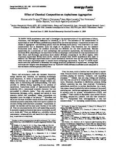
The sixth function is used for the communication of the rigid bodies’ information. Just as some particles’ information is shared by neighboring GPUs, the rigid bodies’ information also should be communicated between GPUs every time step. The communication of the rigid bodies’ information should be accomplished before the communication of the particles’ information. Fig. 1 shows the serial algorithm of this part. The Particle counter is determined in the function for the calculation of the torque and the linear velocity, and the number of outgoing particles is determined in the function for dealing with the particles that crossed a subdomain border [26]. In our implementation, the code in the loop was parallelized. For the rigid body that consists of N particles, if the value of the particle counter is equal to N, it means the rigid body was located in the subdomain entirely before the positions updated. In this way, the properties data of the rigid body should be collected and sent to the neighboring GPU if there are any particles moving out of the subdomain at this time step. The communication is very important although the amount is usually small. 3. Performance Simulations of the heavy crude oil system were performed on different kinds of GPU devices in order to evaluate the performance. The GPU devices are Tesla C1060, Tesla C2050, GeForce GTX480 and GeForce GTX690. The C1060 is based on GT200 architecture and the peak performance is about 933 GFlops in single precision. The C2050 and the GTX480 are based on Fermi architecture, and both of them have more than 400 CUDA cores. The C2050 has the error correcting code (ECC) to safeguard the memory against corruption, and its performance for the double precision calculations is significant. Compared with the C2050, the GTX480 has higher performance for the single-precision floating-point calculations. Our previous work has present that simulations of quite large systems can be performed on the GTX480 very efficiently. The GTX690 are a dual GPU device based on NVIDIA s new Kepler architecture. For a single GPU of the GTX690, memory clock and performance for the single-precision floating-point calculations are

improved to about 3TFlops and 6000 MHz respectively. Details of the heavy crude oil system were described in the simulation section. Each simulation was performed for 10,000 time steps, and the average time steps per second were calculated. Fig. 2 shows the performance obtained while performing simulations of different-sized systems on each GPU device. For comparison, performance of the serial program was tested on the Intel Q9400 CPU. The simulation system sizes in the test are 20 ∗ 20 ∗ 20, 40 ∗ 40 ∗ 40 and 60 ∗ 60 ∗ 60. In Zhang’s work, it took more than a week to calculate the diffusion coefficient of asphaltene in toluene by performing simulations of a 60 ∗ 60 ∗ 60 system. This figure indicates the high speedup of our implementation. For simulations of a 60 ∗ 60 ∗ 60 system, our GPU-accelerated implementation achieved 20x–50x speedup using a single GPU. Our previous work has proved that GPU worked more efficiently when the simulation system became larger [26]. As Fig. 2 shows, the time consumed by performing simulations of quite large systems is still acceptable. In addition, GPU devices have a significant influence on the performance of our implementation because of the distinct different computational power. For simulations of large systems, GPU devices based on Fermi architecture can run about 2 times faster than the C1060. It is also obvious that the GTX480 outperforms the C2050. The reasons are the more CUDA cores and higher GPU clock of the GTX480 and the ECC of the C2050 which may slightly slower the memory access speed. Although the program code was not written specifically to match Kepler architecture, the test showed that using the GTX690 achieved the highest performance. A single GPU of the GTX690 can run about 3.3 times faster than the C1060 in the simulation of a 100*100*100 system. Fig. 2 also indicates the performance improvement brought by using 2 GPUs of the GTX690 in parallel. As the simulation system size increases, this improvement becomes more and more pronounced. Fig. 3 shows the performance obtained while performing simulations of the heavy crude oil system and the single particle system on different number of the C2050 GPUs. The simulation system size is 120 ∗ 120 ∗ 120, which is large enough to make the distribution of computational load well-balanced no matter how many GPUs are used. It is obvious that the performance keeps improving as the number of GPUs increases. Compared with the performance of using a single C2050 GPU, our implementation running on 6 C2050 GPUs in parallel can be about 4.5 times faster. For simulations of the heavy crude oil system, there are more than 100,000 rigid bodies and a huge number of spring force interactions. The process of the rigid body rotation and the spring force calculation can increase the computation time of GPUs. Besides, the global synchronization with a barrier function provided by POSIX has to be

S. Wang et al. / Computer Physics Communications 185 (2014) 3069–3078

3073

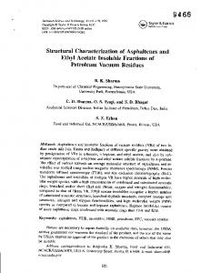
Fig. 4. Average coarse-grained DPD molecules of the compounds in the heavy crude oil. Gray particles are side chains (Type B). Functional groups containing heteroatoms (Type C) are given in purple. Three colors are used for type A particles, red for the rigid moiety of asphaltenes, green for resins, and black for aromatics. (For interpretation of the references to color in this figure legend, the reader is referred to the web version of this article.) Fig. 3. The comparison of performances obtained while performing simulations of the heavy oil system and the single particle system. The simulation system size is 120 ∗ 120 ∗ 120.

made more often in each time step of the simulation. Accordingly, the performance obtained in simulations of the heavy crude oil system is slightly slower than that of the single particle system. 4. Simulations The benchmark test presents that our implementation has a high performance for simulation of systems containing rigid bodies on GPU. By using our workstation equipped with 6 C2050 GPUs, performing simulation of significant large systems at long time scales is available. In this section, by simulations of the heavy crude oil system, the asphaltene–toluene system and the asphaltene–heptane system, the diffusion and aggregation of asphaltenes are studied and discussed. The coarse-grained model molecules and conservative force parameters that we used in all simulations are the same as that in Zhang’s work [17]. According to the relationship between parameters in DPD and χ -parameters in Flory–Huggins theory [31], the conservative force parameters were determined by the Blends method with slight adjustments. We employed 3 types of particles to construct the model molecules, A, B and C. Type A represents the moiety of aromatic rings, type B for the alkyl chain and type C for the functional group containing heteroatoms. Structures of the model molecules are shown in Fig. 4. Three colors are used for particles of type A to benefit the detection of specific fractions from the simulation results. The model molecule for heptanes is also used for the light fraction. For all simulations, the dimensionless temperature T is initialized as 1.0, and the particle density is set to 3 [31]. According to the fluctuation–dissipation theorem [32], we choose the noise parameter σ = 3, and the dissipative parameter γ = 4.5 [31]. At the beginning of each simulation, most particles are distributed arbitrarily and evenly in the simulation box. 4.1. The heavy crude oil system In order to validate our implementation, simulations of the heavy crude oil system were performed and the simulation results were compared with that in Zhang’s work [17,18]. A 120 ∗ 120 ∗ 120 system was used, the mass ratio of five fractions of heavy crude oil (asphaltenes:resins:aromatic:saturate:light fractions) is 1:3:3:2:17. The time step size was set to 0.01, and 300,000 time steps of simulation were performed. Fig. 5 shows the nanoaggregates formed by associated asphaltene molecules in the system. Most nanoaggregates have a

well-ordered structure formed by a number of interior fused aromatic rings and exterior side chains. The side chains of asphaltene molecules act as the repulsive part by a steric hindrance effect and repel additional asphaltene molecules. Therefore, resin molecules do not participate in forming the nanoaggregates but just surround them. In addition, some larger aggregates consist of more than one nanoaggregate, which can be identified as clusters. From this figure, the features of aggregate structure in heavy oil that our simulation presented are similar to that in Zhang’s work [17,18]. Fig. 6 shows the MSD of each fraction of heavy crude oil, which also agree well with that in Zhang’s work [18]. The slop of the MSD curve for each fraction can reflect the diffusivity. Since most asphaltene molecules aggregate to form nanoaggregates and they have the largest molecular weight, the slop is the lowest. Resin molecules are around the asphaltene nanoaggregates and move with them, which can explain why the MSD curves for asphaltenes and resins are very close to each other. In addition, due to the wellproportioned dispersed status and lighter molecular weight of aromatics and saturates, the slops of them are relatively large. Compared with Zhang’s work, the consistency of simulation results proved the accuracy and the validity of our implementation. Moreover, the statistical analysis of the simulation performed on multiple GPUs can be more meaningful. In Zhang’s work, the MSD curve for asphaltenes fluctuates strongly because the number of asphaltene molecules in the simulation system is quite small. In contrast, since the simulation system in this work is large enough to contain a great number of molecules of each fraction, the MSD curves in Fig. 6 are almost straight lines without obvious fluctuation. 4.2. The asphaltene–toluene system As we know, toluene is a suitable solvent for asphaltenes. At relatively low concentrations, asphaltenes exist as monomers and nanoaggregates in toluene solvent. Measuring the diffusion coefficient (D) of asphaltenes can assist in studying asphaltene monomers and the aggregates. Different values of D for dilute asphaltene solutions have been reported by carrying out various experimental investigations. Andrews et al. [33] used fluorescence correlation spectroscopy to study asphaltene molecules in toluene at extremely low concentrations, and they found that the translational diffusion coefficient was about 3.5 × 10−10 m2 s−1 at room temperature. By using the nuclear magnetic resonance methods, Lisitza et al. [8] discussed the relationship between D of asphaltenes in toluene and concentration. At low concentrations (below 0.2 g L−1 ), their study gave a constant D = 2.9 × 10−10 m2 s−1 .

3074

S. Wang et al. / Computer Physics Communications 185 (2014) 3069–3078

Table 1 Simulation schemes for the asphaltene–toluene system.

S1 S2 S3 S4 S5 S6 S7 S8 S9 S10 S11

Simulation system size

Number of asphaltene molecules

Number of toluene molecules

Concentration of asphaltenes (g L−1 )

80 ∗ 80 ∗ 80 80 ∗ 80 ∗ 80 100 ∗ 100 ∗ 100 100 ∗ 100 ∗ 100 100 ∗ 100 ∗ 100 120 ∗ 120 ∗ 120 120 ∗ 120 ∗ 120 150 ∗ 150 ∗ 150 150 ∗ 150 ∗ 150 150 ∗ 150 ∗ 150 180 ∗ 180 ∗ 180

400 300 400 300 200 300 200 300 200 100 100

508 667 509 500 996 667 997 500 998 333 1725 500 1726 333 3372 500 3373 333 3374 167 5831 167

5.64 4.23 2.89 2.17 1.45 1.26 0.83 0.64 0.42 0.22 0.12

Fig. 5. The snapshot of aggregate structure in heavy crude oil. The asphaltene, resin, aromatic and saturate molecules are red, green, black and gray, respectively. The light fraction molecules are not displayed. (For interpretation of the references to color in this figure legend, the reader is referred to the web version of this article.)

Fig. 6. The MSDs of five fractions in the heavy oil system.

At the higher concentrations (above 0.3 g L−1 ), a continuous decrease of D to 1.0 × 10−10 m2 s−1 was observed. Calculating the slope of Mean-square displacement (MSD) in DPD simulation can also be used to determine the diffusion coefficient: D = lim

1 

|r(t ) − r(0)|2



(21) 6t where r(t) is the relative displacement of the particle at a given time t, and r(0) is the particle’s initial position. In Zhang’s work, the diffusion coefficient of diluted asphaltenes in toluene determined from the simulation is similar to that found experimentally [18]. The concentration of asphaltenes in the most dilute system was 0.43 g L−1 , and the corresponding D was about 1.4 × 10−10 m2 s−1 . t →∞

However, the sizes of all simulation systems in his work are small because of the serial DPD program’s low performance. Therefore, the MSD curves for asphaltenes are quite unstable, and the accurate slope is hard to calculate. In addition, D of asphaltenes at lower concentrations was not determined. In this work, our GPU-accelerated implementation was used to study D of asphaltenes in toluene at extremely dilute concentrations. Details of simulation schemes are shown in Table 1. To achieve better statistical analysis results, the number of asphaltene molecules in each simulation system is larger than 100. The density of each simulation system is approximately equal to the density of toluene at 273 K, which was taken as 866.9 g L−1 . Based on the mass ratio of the binary mixture of asphaltenes and heptane, the values of concentrations in table were calculated roughly. For a 180 ∗ 180 ∗ 180 simulation system that contains 100 asphaltene molecules, the corresponding concentration of asphaltenes is about 0.12 g L−1 . This value is much lower than the most dilute concentration in Zhang’s work [18]. Here the time step size was set to 0.01, and 500,000 time steps of simulation were performed. All calculated diffusion coefficients of asphaltenes versus concentration are showed in Fig. 7. At the most dilute concentration, the value of D is about 2.0 × 10−10 m2 s−1 , which is slightly smaller than the experiment result. An explanation is that the model molecule we use is not precise enough, especially for toluene. Both the relative molecular mass and the radius of gyration of the model molecule for toluene are larger than that of the real toluene molecular. Overall, the calculated diffusion coefficients of asphaltenes are all of the same order as obtained experimentally. In addition, the displayed relationship between D of asphaltenes and concentration is similar to that in Lisitza’s work [8]. At low concentrations, D of asphaltenes is large since most monomers and a few nanoaggregates are present in toluene. With the increasing of concentration, D decreases since larger and larger aggregates are formed.

S. Wang et al. / Computer Physics Communications 185 (2014) 3069–3078

Fig. 7. Diffusion coefficient versus concentration.

3075

Fig. 8. The z-average aggregate size during the simulation of a 40 ∗ 40 ∗ 40 system that contains 200 asphaltene molecules. The concentration is about 17.68 g L−1 .

The model molecule for asphaltenes can be assumed to be a sphere. Therefore, the diffusion coefficient approximately follows a linear relationship with the inverse of the viscosity according to the Einstein–Stokes equation [34] D=

kB T

(22)

6π µR

where D is the diffusion constant, kB is the Boltzmann’s constant, T is the temperature, µ is the solvent viscosity, and R is the radius of the sphere. For each simulation, the radius of gyration of the asphaltene molecule has been recorded. All calculated values of the root mean square radius of gyration are about 1.7. In addition, since the concentration of each simulation system is very dilute, the viscosity can be described as a function of the volume fraction according to the Einstein’s equation [35]. Consequently, there is a roughly linear relationship between the diffusion coefficient of asphaltenes and the inverse of the concentration. Based on this relationship, the curve used the nonlinear fitting method is displayed in figure. Fig. 9. Z -average aggregate sizes at dilute concentrations.

4.3. The asphaltene–heptane system Compared with the asphaltene–toluene system, asphaltene molecules have stronger tendency to form aggregates in heptane. To study the aggregation behavior of asphaltenes, simulations of the asphaltene–heptane system were performed by using our GPU-accelerated implementation. 23 simulation schemes were arranged. Concentrations reduces from about 17.68 g L−1 to 0.10 g L−1 by increasing the size of simulation box. Like simulations of the asphaltene–toluene system, at least 100 asphaltene molecules were in each simulation system. We use a time step of 0.02 for 500,000 steps, and record the z-average aggregate size Sz at intervals of 1000 steps as the index number to study the aggregates. Sz was calculated from Eq. (23) where ni is the number of aggregates i containing gi monomers.



ni gi3

i

Sz = 

ni gi2

.

(23)

i

MD simulation has been used to study the asphaltene–heptane system by Sedghi et al. [15], and the simulation results predict three distinct stages of aggregation as proposed by the modified Yen model during the simulation. In this work, much larger spatial and temporal scale systems were studied by DPD simulation. For

the DPD simulation of a 40 ∗ 40 ∗ 40 system that contains 200 asphaltene molecules (17.68 g L−1 ), similar results were found. Fig. 8 shows the average aggregate size of asphaltenes during the simulation. Since asphaltene molecules are evenly distributed at the beginning of the simulation, there is no initial formation of aggregates. Sz increases to about 10 after a small number of time steps, which means nanoaggregates are formed quickly. After 100,000 time steps, nanoaggregates start to form clusters with Sz > 20. Since the concentration of asphaltenes is relatively high, asphaltene flocculation can be observed finally. Sz increases to more than 110 at the end of the simulation. The system separates into two distinct phases at this stage. Fig. 9 shows the z-average asphaltene aggregate size of each simulation system at relatively low concentrations of asphaltenes. Sz is smaller than 2 when concentrations are lower than 0.2 g L−1 , which means most of the asphaltene molecules exist as monomers in heptane. When concentrations are above 0.3 g L−1 , Sz increases from 3 to 6. In this concentration range, asphaltene molecules tend to form nanoaggregates. Some experimental works have shown that the different asphaltenes have somewhat different values of CNAC. For the sample that was extracted from UG8 crude oil, both high-Q ultrasonics [5] and DC conductivity [7] show that the CNAC for asphaltenes in toluene is about 0.15 g L−1 . For the sample that was extracted from BG5 crude oil, the CNAC determined by

3076

S. Wang et al. / Computer Physics Communications 185 (2014) 3069–3078

Fig. 10. The z-average aggregate size versus concentration.

DC conductivity is about 0.06 g L−1 . At dilute concentrations, determining the exact value of CNAC by DPD simulation is difficult. Nevertheless, from Fig. 9 we can see that the CNAC for asphaltenes in heptane determined by our simulation is around 0.2 g L−1 to 0.3 g L−1 . Fig. 10 gives the relationship between z-average asphaltene aggregate size and concentration from all the simulation results. Aggregates become larger in heptane with increasing concentra-

tions. According to the modified Yen model, nanoaggregates have small aggregate sizes (