Jack E. Juni l, James H. Thrall 2, Jerry W. Froelich 2 Roger C. Wiggins 3, Darrell A. Campbell, Jr 3, and Michael ... 2 Henry Ford Hospital, Detroit. Michigan, USA.
European M I I~lt~cir Journalof I ~ i l U ~ t ~ / l ~ , f . . 4 /
Eur J Nucl Med (1988) 14:403-407
Medicine © Springer-Verlag 1988
The appended curve technique for deconvolutional analysismethod and validation Jack E. Juni l, James H. Thrall 2, Jerry W. Froelich and Michael Tuscan 3
2 Roger
C. Wiggins 3, Darrell A. Campbell, Jr 3,
1 William Beaumont Hospital, Department of Nuclear Medicine, 44201 Deqmndre Road, Troy, MI 48098-1198, USA 2 Henry Ford Hospital, Detroit. Michigan, USA 3 University of Michigan Medical Center, Departments of Internal Medicine and Surgery, Ann Arbor, Michigan, USA
Abstract. Deconvolutional analysis (DCA) is useful in correction of organ time activity curves (response function) for variations in blood activity (input function). Despite enthusiastic reports of applications of DCA in renal and cardiac scintigraphy, routine use has awaited an easily implemented algorithm which is insensitive to statistical noise. The matrix method suffers from the propagation of errors in early data points through the entire curve. Curve fitting or constraint methods require prior knowledge of the expected form of the results. DCA by Fourier transforms (FT) is less influenced by single data points but often suffers from high frequency artifacts which result from the abrupt termination of data acquisition at a nonzero value. To reduce this artifact, we extend the input (i) and response curves to three to five times the initial period of data acquisition (P) by appending a smooth low frequency curve with a gradual taper to zero. Satisfactory results have been obtained using a half cosine curve of length 2 3P. The FTs of the input and response I and R, are computed and R/I determined. The inverse FT is performed and the curve segment corresponding to the initial period of acquisition (P) is retained. We have validated this technique in a dog model by comparing the mean renal transit times of 13li_iodohippuran by direct renal artery injection to that calculated by deconvolution of an intravenous injection. The correlation was excellent (r= 0.97, P < 0.005). The extension of the data curves by appending a low frequency "tail" before DCA reduces the data termination artifact. This method is rapid, simple, and easily implemented on a microcomputer. Excellent results have been obtained with clinical data.
Key words: Deconvolution - Pharmacokinetics - Transit time - Filters - Algorithm
Quantitative measurements of tracer kinetics are an important part of nuclear medicine. The dynamic pattern of tracer activity over a given organ may be influenced by many factors other than the function of that organ. Quality of bolus injection, systemic recirculation of tracer, and multicompartmental removal of blood pool activity all may potentially alter or distort the temporal pattern of activity seen at the organ of interest. These complicating factors Offprints requests to. J.E. Juni
hamper, and may defeat, attempts to accurately assess isolated organ function. Deconvolutional analysis is a mathematical technique which can correct an organ's time activity curve for the dynamically changing pattern of blood pool activity being presented to that organ. Several techniques of deconvolution have been described in the medical literature (Valentinuzzi and Montaldo 1975; Williams 1979; Kenney etal. 1975; Alderson et al. 1979; Gamel et al. 1973; Nakamura etal. 1982; Kuruc et al. 1983) each with disadvantages which have hindered routine clinical use. We have developed and validated a method of deconvolutional analysis which provides excellent results with clinical scintigraphic data. We have also investigated the correlation of organ impulse response functions (IRF) obtained in-vivo by deconvolution following intravenous and direct intra-arterial injection of tracer.
Methods Deconvolution of scintigraphic data by the division of Fourier transforms has been reported by several groups (Alderson et al. 1979; Gamel et al. 1973; Kuruc et al. 1983). Unfortunately, the abrupt termination of data collection while organ radioactivity remains at a nonzero value results in an sharp discontinuity in the data curves. This discontinuity results in high frequency artifacts in the computed IRF. In order to reduce this artifact, we have developed a modification of the Fourier transform technique. This technique is illustrated graphically in Figs. 1 and 2. Figure 1 a shows an example pair of time activity curves derived from a 99mTc-disofenin hepatobiliary study. Data was collected at = 1 min intervals for 32 min. The blood pool or input function curve was derived from a region of interest over the heart. The liver time activity curve is used as the response function. Figure I b shows the original data curves from Fig. 1 a on an expanded time scale of 0-256 min. The abrupt discontinuity at the end of data collection is clearly seen._ : A smoothly tapering, low frequency curve is appended to each of the original data curves in such a manner as to make the curves gradually and smoothly taper to zero (Fig. 2a). This lengthens the original curve several fold. The shape of the appended curve or tail is not particularly critical and is choosen to consist primarly of very low frequencies relative to the original data and to provide a smooth transition with the terminal points of the original data. We have found that a raised one-half cosine wave with an initial
404
heart (blood pool)
liver
Fig. 1. a Time activity curves derived from the heart and liver following intravenous injection of 99mTc-disofenin (DISIDA). Data was collected at 1 min intervals for 32 min. b Same data as shown in Fig. 1 a but on an expanded time scale of 0-256 min. The abrupt continuity caused by termination of data acquisition is evident, e Result of deconvolution of the curves in Fig. 1 a by direct division of Fourier transforms. Note the large artifact caused by the abrupt termination of data collection
a
amplitude equal to that of the terminal points of the original data series gives good results. In general, as the tail is made longer, the high frequency artifact in the resulting computed I R F is further reduced. As a minimum, an appended curve of at least three times the original data series is usually required. The Fourier transforms o f the resulting extended curves are calculated by a standard fast Fourier transform (FFT) algorithm (Cooley and Tukey 1965). The resulting frequency domain organ curve is divided by the frequency domain blood pool curve. An inverse Fourier transform is performed yielding a time domain curve several times longer than the original data curves. The initial portion of this curve, representing the actual period of data collection, is the computed impulse response function. The remainder of the curve is ignored. Figure 2 b shows the resulting impulse response function displayed on the original time scale of 0-32 min. Simulation study. In order to compare this "appended curve" technique to other methods of deconvolution described in the medical literature, a simulation study was performed. A gamma variate function was generated to simulate an ideal organ impulse response function. An idealized blood pool curve was generated from a different gamma variate function with added re-circulation. The organ response was then simulated by convolving the blood pool and organ impulse response curves. R a n d o m noise was added to both the simulated blood pool and simulated organ curve in a Poisson distribution to simulate the statistical noise encountered in a typical scintigraphic study. The amount of noise added was calculated assuming an average count rate of 1000.2000 counts per point with a peak of 6000 counts. The impulse response function (IRF) was calculated from this noisy data by the appended curve technique as well as by two techniques previously employed in the medical literature, discrete deconvolution by the matrix inversion method of Valentinuzzi and Montaldo (1975) and direct division of Fourier transforms as used by Alderson et al. (1979), with and without use of a lowpass smoothing filter. The I R F calculated by each of these techniques was compared to the original noise free simulated impulse response function and the root mean squared error was calculated. This process was repeated 50 times for each technique. Since most clinical trials of deconvolution have used extensive data smoothing, the discrete matrix inversion method and the appended curve method were also evaluated after first smoothing each noise added curve three times with a standard three point weighted (1-2-1) smoothing algorithm. The average error in calculation of the I R F by each technique is shown in Table i. In-vivo validation. The I R F obtained by deconvolution after
intravenous injection of tracer would be expected to mirror Table t. Computer simulation of noisy data root mean squared
error _+1 S.D.
b Fig. 2. a The original data curves from Fig. I are extended by appending a smoothly tapering, low frequency curve. Time scale 0-256 rain. b Results of deconvolution by the appended curve method. Time scale 0-32 rain
Unsmoothed
Smoothed
Matrix method
Fourier transform
Fourier transform + Tail
>1033
9.10_+13.9 2.1 _+ 5.3
0.87_+1.12 0.35+0.28
2.9_+20.6
405 1-131 Hippuran
the pattern seen with direct arterial injection into an organ. The appended curve technique was validated by examining this correlation in a dog kidney model. As part of an unrelated study, each dog had one kidney removed. A n indwelling catheter was placed directly in the renal artery of the remaining kidney, under conditions where patency of the catheter was maintained by constant infusion of 0.15 gl/hour NaC1 from a freon driven implanted pump. Animals were studied several days after surgery as previously described (Campbell et al. 1983). When renal functions were stable each dog was anethetised with intravenous sodium pentobarbital. Each animal received a rapid bolus intra-arterial injection of 0.125 mCi (4.63 mBq) 131I-ortho-iodohippurate. Sequential g a m m a camera images of the kidney were obtained on a minicomputer at 15 s intervals beginning 1-2 min prior to injection and continuing for 30 min. A renal region of interest was defined and the renal time activity curve generated. This curve represents a direct physical measurement of the renal IRF. Thirty mins after completion of the intra-arterial study, the animal was reinjected intravenously with 0.25 mCi (9.25 mBq) 131I-ortho-iodohippurate. One region of interest was defined over the heart and another over the kidney. Time activity curves were then generated for the blood pool and kidney. After several applications of a three point weighted smooth to the renal time activity curve, deconvolution was performed by the appended curve technique to calculate the renal impulse response function. A total of five combined intra-arterial and intravenous studies were performed. The mean transit time of tracer through the kidney was calculated for both the directly measured and the calculated renal impulse response function by dividing the area under the I R F curve by the height of the curve.
Fig. 4. Measured and calculated time activity curves obtained from a dog suffering from drug induced renal dysfunction. The order of curves is similar to that in Fig. 3
Results
Fig. 5. Correlation of 131I-hippuran mean transit times calculated from direct renal artery injection and from intravenous injection with deconvolution performed by the appended curve technique (r =0.97, P