The Applicability of Breakpoint Detection Methods Using ... - MDPI

remote sensing Article

Monitoring Forest Dynamics in the Andean Amazon: The Applicability of Breakpoint Detection Methods Using Landsat Time-Series and Genetic Algorithms Fabián Santos 1,2, *, Olena Dubovyk 1 and Gunter Menz 3,† 1 2 3

* †

Centre for Remote Sensing of Land Surfaces (ZFL), University of Bonn, Walter-Flex Str. 3, 53113 Bonn, Germany; [email protected] Center for Development Research (ZEF), University of Bonn, Walter-Flex-Str. 3, 53113 Bonn, Germany Remote Sensing Research Group (RSRG), Department of Geography, University of Bonn, Meckenheimer Allee 166, 53115 Bonn, Germany Correspondence: [email protected]; Tel.: +49-(0)228-734-941 Deceased on 9 August 2016.

Academic Editors: Guangxing Wang, Erkki Tomppo, Dengsheng Lu, Huaiqing Zhang, Qi Chen and Prasad S. Thenkabail Received: 31 August 2016; Accepted: 1 January 2017; Published: 12 January 2017

Abstract: The Andean Amazon is an endangered biodiversity hot spot but its forest dynamics are less studied than those of the Amazon lowland and forests from middle or high latitudes. This is because its landscape variability, complex topography and cloudy conditions constitute a challenging environment for any remote-sensing assessment. Breakpoint detection with Landsat time-series data is an established robust approach for monitoring forest dynamics around the globe but has not been properly evaluated for implementation in the Andean Amazon. We analyzed breakpoint detection-generated forest dynamics in order to determine its limitations when applied to three different study areas located along an altitude gradient in the Andean Amazon in Ecuador. Using all available Landsat imagery for the period 1997–2016, we evaluated different pre-processing approaches, noise reduction techniques, and breakpoint detection algorithms. These procedures were integrated into a complex function called the processing chain generator. Calibration was not straightforward since it required us to define values for 24 parameters. To solve this problem, we implemented a novel approach using genetic algorithms. We calibrated the processing chain generator by applying a stratified training sampling and a reference dataset based on high resolution imagery. After the best calibration solution was found and the processing chain generator executed, we assessed accuracy and found that data gaps, inaccurate co-registration, radiometric variability in sensor calibration, unmasked cloud, and shadows can drastically affect the results, compromising the application of breakpoint detection in mountainous areas of the Andean Amazon. Moreover, since breakpoint detection analysis of landscape variability in the Andean Amazon requires a unique calibration of algorithms, the time required to optimize analysis could complicate its proper implementation and undermine its application for large-scale projects. In exceptional cases when data quality and quantity were adequate, we recommend the pre-processing approaches, noise reduction algorithms and breakpoint detection algorithms procedures that can enhance results. Finally, we include recommendations for achieving a faster and more accurate calibration of complex functions applied to remote sensing using genetic algorithms. Keywords: forest dynamics; Landsat time-series; genetic algorithms; breakpoint detection

Remote Sens. 2017, 9, 68; doi:10.3390/rs9010068

www.mdpi.com/journal/remotesensing

Remote Sens. 2017, 9, 68

2 of 27

1. Introduction Since an open data policy was adopted by the Landsat program, an increasing number of data-driven algorithms for monitoring forest dynamics using Landsat time-series (LTS) have been developed [1]. They highlight abrupt events (e.g., clear-cutting, crown fires) or slower processes (e.g., degradation, succession dynamics) that, within a longer time spam, cause deviations or illustrate longer-duration changes from a presumably stable condition [2]. Typically, these algorithms are called breakpoint detection algorithms (BDA), and according to Banskota et al. [3], they can be classified according to their methodological basis and scope. This research establishes breakpoint detection as a useful implementation of LTS analysis; however, conditions in the Andean Amazon—high topographic relief, cloud cover that prevents the production of more than a few clear observations throughout the year, and landscape variability—complicate this type of analysis. Furthermore, pre-processing approaches and noise-reduction algorithms for Landsat have evolved in recent decades [4], making for significant variation in preparing the data it generates to enhance breakpoint detection [5–7]. For this reason, the interpreter’s experience plays an important role in selecting, calibrating, and applying an algorithm. Inappropriate selection or calibration can introduce systematic errors that can be difficult to detect. This problem is particularly overwhelming, with a large number of complex algorithms interlinked. Breakpoint detection requires a dense time-series of Landsat images that are radiometrically homogeneous, free of cloud and shadow, and geometrically corrected. Achieving these levels of processing is challenging since parametrization of these algorithms is not an easy task, and computer-processing LTS data is highly demanding. For these reasons, it has become necessary to optimize the complex processing chains that combine pre-processing, noise reduction, and BDA procedures. There is little research in this field. Nonetheless, optimization has been shown to be successful in remote sensing. Examples vary according to the field and the search algorithm applied [8–10]. Genetic algorithms (GAs) have a long history of refinement since it became popular though the work of Holland [11]; extensive research has reported it as a robust and efficient optimization algorithm with a wide range of application in areas such as engineering, numerical optimization, robotics, classification, pattern recognition, and product design, among others [12,13]. Therefore, we chose a GA as our methodological approach to designing a processing chain based in BDA and to evaluate if this procedure might be a feasible approach for monitoring forest dynamics in the Andean Amazon. Since this is our first step before exploring other complex optimization procedures that, according to Eberhart et al. [14], should be emphasized in the new hybrid implementations, we avoid extending our discussion in search of new algorithms. Such discussion is beyond the scope of this paper. We therefore recommend that interested readers review the references mentioned throughout this paper. Our particular research objective focuses on conducting a GA optimization of different processing chains using different BDA in order to determine if it is possible to monitor the forest dynamics in the Andean Amazon. If the methodology is applicable, patterns of forest gain and forest loss should be evidenced during a period of time along a typical part of the Andean Amazon. Furthermore, since there are multiple methods of enhancing time-series quality, we also analyze different pre-processing approaches and noise reduction algorithms for improving breakpoint detection. In order to do this, we develop a function called a processing chain generator (PCG) to link these approaches as processing chains and evaluate if their results highlight patterns of forest dynamics. Since calibrating the PCG is not straightforward, due to the number of parameters involved in algorithms calibration (24 parameters with a total of 5.7491 × 1020 possible combinations), GA was used as the basis for exploring and designing an optimal calibration for the PCG. For this reason, our research also constitutes a novel approach for solving the calibration of complex models in remote sensing by reducing uncertainties through parametrization. This method is different from other optimization approaches in remote sensing, where the principal application is classification and pattern recognition [8–10]; however, it is closer to the approach of Reference [15] for calibrating a model of cellular automata.


3 of 28

cloud cover, high topographic relief, and different forest management practices along a gradient of altitude. We found that these conditions mean the application of any remote sensing-based methodology is not straightforward. Remote Sens. 2017, 9, 68

3 of 27

2. Materials and Methods As landscape factor monitoring Andean In this this research section, considers we describe general variability aspects of an theimportant study area, the in Landsat data the acquired for Amazon, study areas in Ecuador were selected. They aresince characterized frequent conduct different our experiments, andlocated the validation datasets used. Moreover, a highly by accurate cocloud cover, is high topographic relief, and different management practices a gradient registration required for breakpoint detection, weforest include an assessment of the along Landsat standard terrain correction (Levelthat 1T) these to ensure that images used properlyofco-registered. of altitude. We found conditions mean thewere application any remote sensing-based methodology is not straightforward. 2.1. Study Area 2. Materials and Methods The study area covers in total 241 km2 distributed across three areas of 100, 52, and 89 km2 termed In thisC, section, we describe aspects of were the study area, acquired for conduct A, B, and respectively. Theirgeneral selection criteria based on the the Landsat differentdata landscape configurations our experiments, the validation used. Moreover, since aobserved highly accurate co-registration is along a gradientand of altitude and ondatasets forest management practices in the region. The areas required we include the Landsat standard (Figure terrain correction studied for arebreakpoint located indetection, the central foothillsanofassessment the Napoofprovince in Ecuador 1), where (Level 1T) to ensure that images used were properly co-registered. mountainous terrain, foothills, and lowland evergreen forests constitute the main ecosystems [16].

The principal river is the Napo, which joins the Amazon River after 1800 km. The geomorphology is 2.1. Study Area characterized by hilly (slopes between 0°–26°) and mountainous (slopes greater than 26°) landscapes 2 distributed withThe highstudy biodiversity [17]. in Thetotal altitude covers a range ofacross 300–3875 meters Therefore, area covers 241 km three areasa.s.l. of 100, 52, andthe 89region km2 is characterized distinct climatic gradient withcriteria annual were precipitation of the 2000different mm –4000 mm and termed A, B, andbyC,a respectively. Their selection based on landscape a mean temperature 6 °C–24of°C. The main use systems are grasslands used for cattle configurations along aof gradient altitude and land on forest management practices observed in the grazing region. andareas croplands for cacao, passion fruit, and corn [18]. in The land cover change area, The studiedused are located in the central foothills of theproduction Napo province Ecuador (Figure 1), where which included forest loss andand gain classesevergreen for the period ha [19].[16]. The mountainous terrain, foothills, lowland forests2000–2014, constitute covered the main3862 ecosystems respective study areas measured 324 ha (Area 1575 haRiver (Areaafter B), and (Area C) as a result The principal river is the Napo, which joins theA), Amazon 18001963 km.ha The geomorphology their differentby forest practices. isofcharacterized hillymanagement (slopes between 0◦ and 26◦ ) and mountainous (slopes greater than 26◦ ) Area A (mountainous, 2300–750 a.s.l.) is located in theofvicinity of amprotected area where landscapes with high biodiversity [17].meters The altitude covers a range 300–3875 a.s.l. Therefore, the forest is loss is rare and itby is amainly caused by gradient natural events (landslides or river floods); Area B (mainly region characterized distinct climatic with annual precipitation of 2000 mm–4000 mm ◦ C–24 ◦in hilly, 750–500 meters a.s.l.) of a settlement where forest loss used is common and and a mean temperature of is6 located C. the Thevicinity main land use systems are grasslands for cattle caused and principally byused expansion of the agricultural land; Area C (mainly meters grazing croplands for cacao, passion fruit, and cornand production [18]. Theflat, land500–350 cover change a.s.l.)which is located in a forest privateloss forest whose suffer forest lost as a result of [19]. road area, included andreserve, gain classes forborders the period 2000–2014, covered 3862 ha construction theareas interior is experiencing forest gain ha as (Area a result ecological success some The respective but study measured 324 ha (Area A), 1575 B),of and 1963 ha (Area C) after as a result acquired conservation. ofareas theirwere different forestfor management practices.

Figure1.1.(a) (a)Location Locationof ofstudy studyareas. areas.(b) (b)Photographs Photographsobserved observedatatA, A,B,B,and andCCstudy studyareas. areas.AAisislocated located Figure thevicinity vicinityofofaaprotected protectedarea, area,BBisislocated locatedclose closetotoaasettlement, settlement,and andCCisislocated locatedininaaprivate privateforest forest ininthe reserve,surrounded surroundedby byagricultural agriculturalland. land. reserve,

Area A (mountainous, 2300–750 m a.s.l.) is located in the vicinity of a protected area where forest loss is rare and it is mainly caused by natural events (landslides or river floods); Area B (mainly hilly,


4 of 27

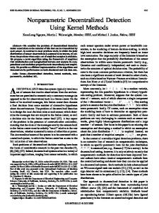
750–500 m a.s.l.) is located in the vicinity of a settlement where forest loss is common and caused principally by expansion of the agricultural land; and Area C (mainly flat, 500–350 m a.s.l.) is located in a private forest reserve, whose borders suffer forest lost as a result of road construction but the interior is experiencing forest gain as a result of ecological success after some areas were acquired Remote Sens. 2017, 9, 68 4 of 28 for conservation. 2.2. Landsat Data Acquisition and Geometry Correction Assesment 2.2. Landsat Data Acquisition and Geometry Correction Assesment For this study, we obtained 826 surface reflectance images for a subset of two Landsat footprints For this study, we obtained 826 surface reflectance images for a subset of two Landsat footprints (path and row: 09–61 and 10–61; total area: ~4400 km22), which were processed through National (path and row: 09–61 and 10–61; total area: ~4400 km ), which were processed through National Landsat Archive Processing System (LEDAPS) [20]. They were downloaded from the US Geological Landsat System (LEDAPS) [20]. They the were downloaded from the US Geological SurveyArchive throughProcessing their Internet website [21]. After applying cloud mask “cfmask” product [22] 677 Survey through their Internet website [21]. After applying the cloud mask “cfmask” product [22] 677 of these images were not used due to low image quality, including excessive no data cover of (>90%) these images notremaining used due149 to low image quality,inincluding excessive no dataacquired cover (>90%) (Figurewere 2a). The images employed this analysis were originally for (Figure 2a). The remaining 149 images employed in this analysis were originally acquired for three three Landsat sensors: 28 images by Thematic Mapper (TM), 94 images by Enhanced Thematic Landsat sensors: 28 images by Thematic Mapper (TM), 94 images by Enhanced Thematic Mapper Plus Mapper Plus (ETM+), and 27 images by Operational Land Imager (OLI). All imagery was processed (ETM+), and 27 images Operational Land (OLI). reported All imagery was processed to the(RMSE) standard to the standard terrainby correction (Level 1T), Imager and metadata a root mean square error of less than 7 ± (Level 3 m. A1T), summary of acquisition parameters forsquare these images is shown in Table The terrain correction and metadata reported a root mean error (RMSE) of less than1. 7± 3 m. images selected for analysis covered an 18-year period (1996–2015) with a mean time interval between A summary of acquisition parameters for these images is shown in Table 1. The images selected for imagescovered of 47 days. analysis an 18-year period (1996–2015) with a mean time interval between images of 47 days.

Figure 2. (a) percentage observed for period 1996–2015 the subset of two Landsat Figure 2. (a) No No datadata percentage observed for period 1996–2015 for thefor subset of two Landsat footprints footprints used (149 images selected). (b) Spatial distribution of no data frequency. used (149 images selected). (b) Spatial distribution of no data frequency. Table1.1.Acquisition Acquisition parameters parameters of Table of the the used usedimages. images. Parameters

Parameters

Sun Azimuth

Range

Range

45°–132°

Average

Standard Deviation

92°

38°◦

Average

Sun Azimuth 45◦ –132◦ 92◦ ◦ Sun Elevation Sun Elevation 53◦53°–62° –62◦ 5858° Crossing time 14:40:08–15:28:42 15:12:50 Crossing time 14:40:08–15:28:42 15:12:50 Cloud cover (%) 19–89 68 Cloud cover (%) 19–89 Time interval between images (days) 1–304 4768 Number of ground control points 9–240 7547 Time interval between images (days) 1–304 RMSE of geometric residuals (meters) 3–11 7

Number of ground control points

9–240

75

RMSE of geometric residuals (meters)

3–11

7

Standard Deviation 38 3° 3◦ 9 min 9 min 16 16 53 49 53 3

49 3

As geometric accuracy of Landsat data is based on its footprint, we considered it necessary to evaluate again foraccuracy our study, as our research sites were than awe footprint. Therefore, we to first Asitgeometric of Landsat data is based on its less footprint, considered it necessary evaluate it again for our study, as our research sites were less than a footprint. Therefore, we first applied a new co-registration to all images to evaluate if geometric accuracy would improve. For this, a Sobel filter was applied to near-infrared channel (band 4) for each image in the LTS. We selected this band because it was less affected by cloud contamination compared to other bands. Then, edge


5 of 27

applied a new co-registration to all images to evaluate if geometric accuracy would improve. For this, a Sobel filter was applied to near-infrared channel (band 4) for each image in the LTS. We selected this band because it was less affected by cloud contamination compared to other bands. Then, edge masks Remote Sens. 2017, 9, 68 5 of 28 were created thresholding these outputs and applying a linear registration to obtain match points and theirmasks transformation matrix. We used an affine that usesa 12 degrees of freedom to find match were created thresholding these outputsmodel and applying linear registration to obtain match points andand thetheir nearest neighbor to resample images. This was that done following theofprocedure points transformation matrix. We used an affine model uses 12 degrees freedom to and find match points and the [23]. nearest resample images. This was done following the in software package of Reference To neighbor establish to a geometric reference, a Landsat 5 image acquired procedure and software package of Reference [23]. To establish a geometric reference, a Landsat 5 November 2000 was selected. For this image, the reported RMSE was 3.4 m with 240 points. To verify image acquired in November 2000 was selected. For this image, the reported RMSE was 3.4 m with if co-registration improves results, displacements were calculated from control points to their new 240 points. To verify co-registration improves results, displacements were calculated control positions. Control pointsif where identified in the reference image as stable areas duringfrom the 19 years of points to their new positions. Control points where identified in the reference image as stable areas the LTS and they are described in Table 2. during the 19 years of the LTS and they are described in Table 2.

Table 2. Acquisition parameters of the used images. Table 2. Acquisition parameters of the used images.

River confluence River confluence Road Property boundary Road

X and and Y X Y Mean Mean Displacements Displacementsin in New Co-Registration (in Meters) New Co-Registration (in Meters) 81.2 81.2 576.4 97.3 576.4

Number of Number of Point Point Matches Matches with Overlap >80% with Overlap >80% 62 62 182 667 182

Property boundary

97.3

667

Study Area Study Area

Control Point Details Control Point Details

A AB BC

C

The results of the described co-registration, however, did not improve the geometric accuracy The results of the described however, did not displacements improve the geometric accuracythus, of the images. On the contrary, the co-registration, new co-registration increased in the images; the was images. On thefrom contrary, the new co-registration displacements in the images; thus, this of step omitted the analysis. In Figure 3,increased the results of the co-registration procedure this step was omitted from the analysis. In Figure 3, the results of the co-registration procedure displacements can be seen as red crosses, while control points as white dots. Results in Table 2 indicated displacements can be seen as red crosses, while control points as white dots. Results in Table 2 that Area C was the easiest to co-register, but it was not enough to replace its existing geometric indicated that Area C was the easiest to co-register, but it was not enough to replace its existing correction. Because of this, we applied other procedure for evaluate co-registration. It consisted in geometric correction. Because of this, we applied other procedure for evaluate co-registration. It addconsisted the edgeinmasks created in thecreated steps before for observe they overlap along the LTS. add the edge masks in the steps before forifobserve if they overlap along theSince LTS. the maximum overlap corresponds to areas where all images it was normalized from 1 (no overlap) Since the maximum overlap corresponds to areas where match, all images match, it was normalized from 1 to 100 imagestoin100 the(all LTS overlaps). pixels whose overlap exceedsoverlap 80% were filtered (no(all overlap) images in theThen, LTS overlaps). Then, pixels whose exceeds 80%(Figure were 3). All three areas showed match except in areaspoints, whereexcept cloud in cover was frequent do not filtered (Figure 3). All threepoints, areas showed match areas where cloudor cover washave frequent or do not borders.in Asthe 20%LTS of the images in the LTS remained uncertain, they and relevant borders. Ashave 20%relevant of the images remained uncertain, they were identified wereinspected identified and visually inspected manually improve their co-registration visually to manually improve to their co-registration or eliminate them.or eliminate them.

Figure 3. Edge maskmask from from reference imageimage (November 2000) 2000) and control, displacements, and matching Figure 3. Edge reference (November and control, displacements, and points with overlap greater than 80% in the: (a) Study area A, (b) Study area B, and (c) Study area C. matching points with overlap greater than 80% in the: (a) Study area A, (b) Study area B, and (c) Study area C.

2.3. Ancillary Data for Sampling, Validation, and Pre-Processing 2.3. Ancillary Data for Sampling, Validation, and Pre-Processing

To establish a land cover change map (LCCM), two maps were created, forest and non-forest. establish a land change map (LCCM), maps created, non-forest. The The timeTo periods used forcover establishing them were two 1997 andwere 2015. Both forest mapsand were obtained using time periods used for establishing them were 1997 and 2015. Both maps were obtained using a triala trial-and-error threshold approach to classify the Natural Burn Ratio (NBR) index derived from the and-error threshold approach to classify the Natural Burn Ratio (NBR) index derived from the first and last images in the LTS. After a visual inspection and correction, these maps were finalized and changes


6 of 27

first and last images in the LTS. After a visual inspection and correction, these maps were finalized and changes between 1997 and 2015 were established corresponding to five classes: stable non-forest, stable forest, forest lost, forest gain, and no data. This map was used later to extract the stratums needed for sampling (training and reference) and to perform visual assessments (Sections 5.3 and 6.4). To validate training and reference samples, a dataset comprised of high-resolution imagery acquired from different sources was used. These images included aerial photos, RapidEye images, Google Earth, and ASTER imagery. These images were acquired for the years 1978, 1982, 2000, 2005, 2010, and 2015. Additionally, a field visit was done during the first semester of 2016 to corroborate the study area’s land cover. Finally, as topographic correction was indicated for Landsat pre-processing, we acquired a digital elevation model (DEM) from the Shuttle Radar Topography Mission (SRTM) [24] with a resolution of 90 m, as its interpolation quality was better than the 30-m version, especially in areas with data gaps of hilly landscapes. 3. Additional Landsat Pre-Processing Calculations Because we need to evaluate different Landsat pre-processing approaches to determine the best calibration of the PCG, we describe in this section all the procedures implemented. These were applied to the subset of two Landsat footprints; therefore, its extension was larger than the study areas. As we calculated different vegetation indices and mosaics ensembles from each Landsat pre-processing approach, we also provide an overview of their procedures. 3.1. Topographic Correction and Radiometric Normalization Topographic correction is considered a fundamental preliminary procedure before multi-temporal analyses because solar zeniths and elevation angles, as well as direct topographic effects, differ from image to image [5]. Both Richter et al. [25] and Riaño et al. [26] concluded that the C-correction method was preferred over other related topographic correction algorithms because it better preserves the spectral characteristics of the imagery. C-correction calculation incorporates the wavelength of each individual spectral band along with its diffuse irradiance. C-correction was originally proposed by Teillet et al. [27], and we applied it to our LTS using the DEM in combination with the solar and azimuth elevation angles described in the imagery metadata. Then, for radiometric normalization, we followed a procedure described by Hajj et al. [28]. This approach applies a relative radiometric normalization based on calculations of linear regressions between target and reference images and uses invariant targets to obtain regression coefficients. An important advantage of this technique is based on its absolute calculations. Vermote et al. [29] described this methodology within the context of the 6S model. The 6S model relies on atmospheric data to reduce the effects of atmospheric and solar conditions relative to a reference image. Another advantage of this procedure is its ease of implementation and computation. To implement radiometric normalization, a nearly cloud- and haze-free OLI surface reflectance image acquired by Landsat 8 on 2 September 2013 was used as reference. Its date corresponds to the low regional precipitation regime (with monthly rainfall below 250 mm) in the region [30]. As with all other images used, this reference image was cloud-masked and dimensionally homogeneous with the rest of the images. Afterwards, invariant target masks were generated from a Normalized Difference Vegetation Index (NDVI) ratio, where the NDVI of the target image was divided by the NDVI of the reference image [31]. In most change detection algorithms, the separation of no-change pixels is based on a histogram of outputs, where the mean or median value is used as the benchmark to define its range [32]. This principle was observed in the NDVI ratio outputs and was implemented by computing different possible ranges in a loop calculation. This operation started from the mean value of the NDVI ratio, and the minimum and maximum values increased by a factor of 0.1% in each loop iteration. The process terminated when the number of pixels within the range exceeded 2% of the total number of pixels in the NDVI ratio. This percentage was considered sufficient to represent


7 of 27

a wide diversity of features: primary forests, bare soils, water bodies, and urban infrastructures, among Hajj Remoteothers. Sens. 2017, 9, 68et al. [28] and Mahiny and Turner [33] both applied percentages below 1% 7 ofwith 28 the recommendation that this figure should be increased as much as possible. Finally, the range was used according toto each image invarianttarget targetmasks. masks.After Afterthe the calculation used according each imagetotoreclassify reclassifyand and create create the invariant calculation of invariant target masks for each in the total), the regression coefficients were of invariant target masks for each targettarget imageimage (148 in(148 total), regression coefficients were calculated calculated a linear For this step, we applied the mask invariant maskand to target the using a linear using regression. Forregression. this step, we applied the invariant target to thetarget reference reference and target images then calculated the for regression coefficients forband. each image’s spectral images and then calculated theand regression coefficients each image’s spectral In this procedure, band. In this procedure, eachimages of the surface reflectance images normalizes its values according each of the surface reflectance normalizes its values according to the reference image. to the reference image. To evaluate the performance of topographic correction, radiometric normalization and other To evaluate thepre-processing performance ofapproaches, topographicdifferent correction, radiometric normalization and for other combinations of these time-series boxplots were made each combinations of these pre-processing approaches, different time-series boxplots were made for each case (Figure 4a). These plots used a sample set of 1678 pixels taken with a precision of 99%. They were case (Figure 4a). These plots used a sample set of 1678 pixels taken with a precision of 99%. They were randomly taken from the predominantly sun-exposed (839 samples, azimuth range areas: 45◦ –132◦ ) randomly taken from the predominantly sun-exposed (839 samples, azimuth range areas: 45°–132°) and and shadowed areas (839 samples, azimuth range areas: 225◦ –313◦ ) (Figure 4b). Since variance should shadowed areas (839 samples, azimuth range areas: 225°–313°) (Figure 4b). Since variance should be be similar in both sun-exposed and shadow-exposed areas if LTS achieves its temporal homogeneity, similar in both sun-exposed and shadow-exposed areas if LTS achieves its temporal homogeneity, the standard deviation was calculated for each case. We obtained measurements of 0.11 for surface the standard deviation was calculated for each case. We obtained measurements of 0.11 for surface reflectance (REF), 0.11 and 0.07 0.07for forradiometric radiometricnormalization normalization reflectance (REF), 0.11for fortopographic topographiccorrection correction (TOPO), (TOPO), and of of surface reflectance (NREF); and 0.15 for radiometric normalization of topographic correction (NTOPO). surface reflectance (NREF); and 0.15 for radiometric normalization of topographic correction Based on these values, it wasvalues, established the NREF pre-processing approach reduced LTSreduced temporal (NTOPO). Based on these it wasthat established that the NREF pre-processing approach variability, whilevariability, other approaches, such as REF, TOPO NTOPO, it. increased it. LTS temporal while other approaches, such and as REF, TOPOincreased and NTOPO,

Figure 4. 4. (a)(a) Examples usingyearly yearlymosaics mosaicsand andthethe NBR Figure Examplesofofdifferent differentpre-processing pre-processing approaches approaches using NBR vegetation index. Boxplots sun-exposedand andshadow shadowareas. areas.Red Red lines vegetation index. Boxplotswere werebased basedin insamples samples located located at sun-exposed lines highlight mean values thetime-series. time-series.The The acronyms acronyms on the surface reflectance; highlight mean values ininthe the right rightstand standfor: for:REF REForor surface reflectance; TOPO or topographic correction;NREF NREFor orradiometric radiometric normalization normalization of and NTOPO TOPO or topographic correction; ofsurface surfacereflectance; reflectance; and NTOPO or radiometric normalizationofoftopographic topographiccorrection. correction. (b) Blue or radiometric normalization (b) Map Map of ofthe thesamples samplesused usedininboxplots. boxplots. Blue dots identify shade-exposedsamples samples while red samples. dots identify shade-exposed reddots dotsidentify identifysun-exposed sun-exposed samples.

Vegetation Indices Derivatives 3.2.3.2. Vegetation Indices Derivatives With the pre-preprocessing outputs, a set of vegetation indices based on visible and infrared With the pre-preprocessing outputs, a set of vegetation indices based on visible and infrared bands bands was calculated. Selection criteria were based on a literature review, considering the was calculated. Selection criteria were based on a literature review, considering the atmospheric effects atmospheric effects described by References [34,35]. Moreover, because the time-series was based on described by References [34,35]. Moreover, because the time-series was based on the surface reflectance the surface reflectance Landsat products, Tasseled Cap Transformations (TCTB, TCTG, and TCTW) Landsat products, Tasseled Cap Transformations (TCTB, TCTG, and TCTW) were applied using the were applied using the coefficients described by Baigab et al. [36]. The indices calculated can be coefficients by Baigab et al. [36]. The indices calculated can be classified in three groups: classified described in three groups: •

Using red and infrared bands: the NDVI [31], Global Environmental Monitoring Index (GEMI) [37], and Modified Soil Adjusted Vegetation Index (MSAVI) [38];


• • •

8 of 27

Using red and infrared bands: the NDVI [31], Global Environmental Monitoring Index (GEMI) [37], and Modified Soil Adjusted Vegetation Index (MSAVI) [38]; Using only infrared bands: The NBR [39], the Aerosol Free Vegetation Index 1.6 µm band8(AFRI16), Remote Sens. 2017, 9, 68 of 28 and the Aerosol Free Vegetation Index 2.1 µm band (AFRI21) [40]; • Using only infrared bands: The NBR [39], the Aerosol Free Vegetation Index 1.6 µm band Using the complete sensor bandwidth: Tasseled Cap Transformation Brightness (TCTB), (AFRI16), and the Aerosol Free Vegetation Index 2.1 µm band (AFRI21) [40]; Greenness (TCTG), and Wetness (TCTW) [41]. •

Using the complete sensor bandwidth: Tasseled Cap Transformation Brightness (TCTB), (TCTG), and Wetness (TCTW) The Greenness topographic correction procedure can[41]. negatively impact the detection of low-magnitude

changes inThe thetopographic landscape [42]. Therefore, all vegetation indices werethe calculated pre-processing correction procedure can negatively impact detectionfor of each low-magnitude changes in the landscape [42]. Therefore, all vegetation were calculated for each pre-processing approach (REF, TOPO, NREF, and NTOPO) to expandindices the PCG calibration alternatives. approach (REF, TOPO, NREF, and NTOPO) to expand the PCG calibration alternatives.

3.3. Mosaic Calculation 3.3. Mosaic Calculation

Following the calculation of the vegetation indices from the different preprocessing approaches, Following the calculation of theimage vegetation indices from theand different preprocessing output images were mosaicked. The acquisition dates yearly, semesterly, approaches, and trimesterly output images were mosaicked. The image acquisition dates and yearly, semesterly, and trimesterly time periods were the principal considerations in structuring the image mosaic. The one-year time periods were the principal considerations in structuring the image mosaic. The one-year timeframe is appropriate for use with Landsat archive data considering data acquisition limitations and timeframe is appropriate for use with Landsat archive data considering data acquisition limitations the 16-day [2].cycle However, consideration of theofshorter temporalities for mosaics and thesatellite 16-day repeat satellitecycle repeat [2]. However, consideration the shorter temporalities for was necessary to validate this affirmation. mosaics was necessary to validate this affirmation. For this procedure, wewe followed describedbyby Griffiths et [43]. al. [43]. Images For this procedure, followedthe themethodology methodology described Griffiths et al. Images were were selected according to their acquisition date number data gapsincluded includedinineach. each. Images Images with selected according to their acquisition date andand thethe number ofof data gaps less extensive data gaps are preferred withina aparticular particular time As As eacheach image fewerwith andfewer less and extensive data gaps are preferred within timeperiod. period. image is selected, any data gaps are filled with data from alternate images from the same time period. is selected, any data gaps are filled with data from alternate images from the same time period. Twenty yearly mosaics, 37 semesterly mosaics, and 64 trimesterly mosaics were obtained to establish Twenty yearly mosaics, 37 semesterly mosaics, and 64 trimesterly mosaics were obtained to establish different periodicities and time-series arrangements. Figure 5 shows that no data percentages that different periodicities and time-series arrangements. Figure 5 shows that no data percentages that remained after the mosaics were calculated. remained after the mosaics were calculated.

Figure 5. Remaining mosaics temporalities. Figure 5. Remainingno nodata data percentages percentages ininmosaics temporalities.

4. Description of the PCG Functionand andIts ItsAlgorithms Algorithms Integrated 4. Description of the PCG Function Integrated In section, this section, we describe each algorithm integratedininthe thePCG PCGbefore before its its optimization optimization with In this we describe each algorithm integrated with GA. GA. Algorithms were executed in three steps, of which the workflow in shown in Figure 6. Starting Algorithms were executed in three steps, of which the workflow in shown in Figure 6. Starting with with the time-series compilation, all steps are further described below. the time-series compilation, all steps are further described below. 4.1. Step 1: Time Series Compilation

4.1. Step 1: Time Series Compilation

To construct a time-series, the PCG needs to define which one of the pre-processing approaches,

To construct a time-series, thetemporalities PCG needs is to used define one of the approaches, vegetation indices and mosaic in which this operation. Allpre-processing these procedures were vegetation indices and mosaic temporalities is used this operation. All these procedures previously described in Section 3; therefore, we do notinextend their discussion. For the first step in were previously described in Section 3; therefore, we do not extend their discussion. For the first step in the the PCG, combining 4 pre-processing approaches, 9 vegetation indices, and 3 mosaics temporalities; total of 1084 time-series compilation alternatives were available. clear reason to select a total PCG,acombining pre-processing approaches, 9 vegetation indices, With and 3no mosaics temporalities; particular one of these alternatives, tour decision was based on defining a combination of three of 108 time-series compilation alternatives were available. With no clear reason to selectthe a particular elements mentioned before. These combinations among others parameters required by the PCG are one of these alternatives, tour decision was based on defining a combination of the three elements summarized in Table 3. mentioned before. These combinations among others parameters required by the PCG are summarized in Table 3.

Remote Remote Sens.Sens. 2016,2017, 8, x 9, 68

9 of 927of 28

Figure 6. 6. PCG PCG workflow. workflow. Figure


10 of 27

Table 3. Summary of PCG steps, methods, algorithms, packages, parameters, values, steps, and their search space size. Steps

Methods

1: Time series compilation

Random selection

2: Outlier detection and removal 3

3: Gap-filling

4: Signal smoothing 3

Parameters 1

Values

P1: Pre-processing and mosaic temporality

REF, TOPO, NREF, NTOPO

-

Yearly, semesterly, trimesterly

-

P2: Vegetation indices

AFRI16, AFRI21, GEMI, MSAVI, NBR, NDVI, TCTB, TCTG, TCTW

-

Decision

P3: Apply it?

No, LOF, deviation

-

Required for all

P4: Window size

2–5

1

Local outlier factor (LOF)

P5: LOF factor

2–15

2

Deviation-based test (deviation)

P6: Threshold

0–14

1

Decision

P7: Which method?

Interpolation, locf, mean imputation

-

Interpolation

P8: Type

Lineal, spline, stine

-

Observation replacement (locf)

P9: Direction

Forward, backward

-

Mean imputation

P10: Type

Mean, median, mode

-

Decision

P11: Apply it?

No, polynomial, convolution

Local polynomial regression fitting (polynomial)

P12: Degree smoothing

0.5–3

0.19

Savitzky–Golay filter (convolution)

P13: Filter order

1–10

1.3

Decision

P14: Which BDA package?

Changepoint, BreakoutDetection, ECP

-

Required for all

P15: Segment size

3–10

1

P16: Statistical property

Mean, variance, mean and variance

-

P17: Algorithm

PELT, binary segmentation

-

P18: Max breakpoints

0–10

1

SIC, BIC, MBIC, AIC, Hannan-Quinn, Manual

-

0–1

0.01

0–1

0.01

Changepoint 5: Breakpoint detection

P19: Penalty mode P20: Penalty for manual mode BreakoutDetection

ECP 1

Steps

P21: Penalty percentage 4

4

P22: Penalization polynomial

0–2

1

P23: Significance level 4

0–1

0.01

P24: Moment index 4

0.1–2

0.01

Total 2

108

448

54

98

2.245 × 1012

The letter ”P” and number indicates the code used in this manuscript for identify parameters. 2 Refers to the total search space as number of alternatives. 3 Modules are optional in the processing chain. 4 Threshold parameter.


11 of 27

Following the stacked time-series, different noise reduction and gap-filling algorithms could be applied in the PCG. The following sub-sections summarize the available options, their characteristics, parameter space sizes, and developer references. 4.2. Step 2: Noise Reduction and Gap-Filling As the PCG required us to define how and whether to enhance the quality of the compiled time-series, multiple algorithms were integrated in the PCG to enhance breakpoint detection. Here, we describe each of them: 1.

Outlier detection, which constitutes the detection and removal of anomalous values in the time-series. Typically, they constitute cloud and shadow pixels that were not properly masked. This step was considered optional and its principal parameters were window size, which defines the moving window to analyze the time series, and the threshold for sensibility control. In total, 448 alternatives were available in the parameter search space. Two algorithms were available for this step:

• • 2.

Gap-filling, which constitutes the procedure for filling data gaps in the time-series caused by cloud and shadow masking or the Landsat 7 ETM+ sensor scan line error. Gap filling was a compulsory step to enable breakpoint detection. The parameters in this step refer to the different methods and options for its execution. Thresholds were not required, so parameter search space was limited to 54 alternatives. Three algorithms were available:

• •

• 3.

Local analysis, using the local outlier factor algorithm (LOF) [44], which calculates for an object a metric to measure how isolated it is with respect to the surrounding neighborhood. A deviation-based test using the Hampel filter, which calculates the median absolute deviation to find outliers [45].

By interpolation, which estimates new data points with methods such as linear, spline, and stine interpolation [46]. Observation replacement, through which missing values are replaced with a temporally adjacent value—the last observation being carried forward or the subsequent observation carried backward. Mean imputation, which replaces missing values with either median, mean, or mode data values.

Signal smoothing, which enables the increase of signal-to-noise ratio in a time-series and enhances the detection of breakpoints. This step was optional since it is not required in breakpoint detection. For all the algorithms included, only one parameter was required to define a threshold for sensibility control. In total, 98 alternatives constituted the parameter search space. Two algorithms were available:

• •

Local Polynomial Regression Fitting [47], which involves the local fitting of a polynomial surface determined by one or more data points. Convolution, using the Savitzky–Golay filter [48], which fits a linear least-squares low-degree polynomial to successive subsets of adjacent data points.

4.3. Step 3: Breakpoint Detection The ultimate step in the PCG is the detection of breakpoints. After it is executed, the PCG gives as outputs the position of the breakpoints found within the time-series analyzed. For this purpose, three different BDA packages were considered since they were programmed in the open source R language [49] and this made it possible to observe their codes and integrate them easily to the GA used [50]. Other alternatives, such as BFAST [51], was discarded as our LTS was not extensive enough to fit a history model. Based on different approaches, two types of BDA were considered:


1.

BDA based in parametric statistics:

•

2.

12 of 27

Methods for Changepoint Detection package (Changepoint) [52], which implements the detection of changes in mean and/or variance values of a univariate time series based on a normality test or cumulative sums. Additionally, Changepoint requires a penalty approach provided by any of five included automatic methods: Hannan-Quinn or Schwarz (SIC), Bayesian (BIC), Modified Bayesian (MBIC), and the Akaike information criterion (AIC). Finally, it includes three algorithms, but we focus on only two. The first one, called binary segmentation, applies a statistical test to the entire dataset and splits it if a single breakpoint is identified. Afterwards, it repeats this operation until no breakpoints are found. The second, called PELT (pruned exact linear time), is based on the algorithm of Jackson et al. [53] but it reduces computational cost and improves accuracy by using a dynamic programming approach.

BDA based in non-parametric statistics:

•

•

Breakout detection via Robust E-statistics package (BreakoutDetection) [54] is an algorithm based on energy statistics. It implements a novel statistical technique called E-divise with medians for estimate the statistical significance of breakpoints through a permutation test. Its design aims to be robust against anomalies. Non-Parametric Multiple Change-Point Analysis of Multivariate Data package (ECP) [55]. This package constitutes an upgrade of the E-divise algorithm developed by the authors of BreakoutDetection. Its novelty is the use of E-divise together with the E-agglomerative technique to reduce processing time by segmenting data before analyzing it.

To avoid any bias caused by unequal search space sizes between BDA packages, threshold parameter ranges were set to similar sizes. Considering all parameters combinations, a total of 2.2 × 1012 alternatives were available in this step. 5. Genetic Algorithm Implementation Since GA is the search algorithm for analyzing the PCG parameter search space, in this chapter we describe the concept behind it, the sampling needed for its implementation, the associated reference data, the fitness evaluation, and the calibration applied to GA. 5.1. Genetic Algorithms GAs are a class of evolutionary algorithms that include scientific models of evolutionary process and search algorithms [15]. They became popular thanks to the work of John Holland and his colleges during the 1970s [11] and are inspired by principles of natural selection and survival of the fittest. GAs have four principal advantages: the capability to solve complex problems, an emphasis on global searches, the provision of multiple solutions, and parallelism. The workflow of GAs aims at evolving a population of feasible solutions for a target problem, or objective function. A fitness evaluation is then made in which each solution is executed and evaluated for its performance with respect to a validation dataset. This process involves an evolution-directed search in the parameter search space of the objective function to create new solutions. In each new generation, the best solutions are selected, reproduced, and mutated with respect to a set of operators used by the GA:

• • •

Selection: Controls the survival of the best chromosomes according to their fitness value and selects them as parents of a new generation. Elitism: An optional selection rule that selects the best chromosomes directly for the next generations to guarantee their existence. Crossover: An operator that creates offspring of the pairs of parents from the selection step. Its probability determines if the offspring will represent a blend of the chromosomes of the parents.


•

13 of 27

Mutation: Adds random changes to the chromosomes.

Remote Sens. 2016, 8, x

13 of 27

To facilitate computation and gene representation, integer encoding is used by GA. This allows To facilitate computation and gene representation, integer encoding is used by GA. This allows the transformation of discrete and continuous parameter values to integer codes and permits GA the transformation of discrete and continuous parameter values to integer codes and permits GA operators totoexperiment as they theywere weregenes. genes. Since discrete parameters are represented operators experimentwith with them them as Since discrete parameters are represented by by an anexact exactnumber numberofof alternatives, their representation as integer-codes is relatively easy. However, alternatives, their representation as integer-codes is relatively easy. However, for forcontinuous continuousparameters, parameters, necessary subset their ranges steps order facilitate their it itis isnecessary toto subset their ranges byby steps in in order toto facilitate their operation. Therefore, defined according accordingtotothe thesensibility sensibility behavior operation. Therefore,this thisprocess processshould shouldbe be carefully carefully defined behavior of of thethe parameter and the of the the algorithm algorithmanalyzed. analyzed. parameter and theinstructions instructionsprovided providedby bythe the developer developer of Since GA terms require should keep keepin inmind mindthat thatthe thefollowing following terms Since GA terms requirea ahomologation, homologation, the the reader should terms refer to:to: (1)(1) PCG asas objective methodsand andparameter parametervalues values PCG refer PCG objectivefunction; function;(2) (2) all all possible possible methods inin thethe PCG as as search space; accuracyassessment assessmentof ofdetected detected breakpoints breakpoints by (4)(4) any search space; (3)(3) accuracy bythe thePCG PCGasasfitness fitnessevaluation; evaluation; any PCG calibration as chromosome and; (5) a parameter value for any algorithm in the PCG as a gene. For PCG calibration as chromosome and; (5) a parameter value for any algorithm in the PCG as a gene. understanding of these concepts, Figure 7 shows how the PCG integrated with GA. Fora abetter better understanding of these concepts, Figure 7 shows how theisPCG is integrated with GA.

Figure PCG workflow. workflow. Figure7.7. GA GA applied applied to PCG

Depending on the complexity of the objective function, GA can be computing-intensive. In this Depending on the complexity of the objective function, GA can be computing-intensive. In this instance, the GA package [50], which allows for flexible manipulation and analysis of the GA, was instance, the GA package [50], which allows for flexible manipulation and analysis of the GA, was used. This package was developed for a parallel computing environment and has been proven to used. This package was developed for a parallel computing environment and has been proven to solve different cases of optimization problems, such as the Rastringin function, Andrews Sine solve different cases of optimization problems, such as the Rastringin function, Andrews Sine function, function, curve fitting, and subset selection, among others. curve fitting, and subset selection, among others. There are other GA drawbacks. Convergence toward local rather than global optimization can be an infrequent problem. Larger populations and more generations are needed to obtain better


14 of 27

There are other GA drawbacks. Convergence toward local rather than global optimization can be Remote Sens. 2016, 8, x 14 of 27 an infrequent problem. Larger populations and more generations are needed to obtain better results, butresults, this demands large simulations. Moreover, due to GAs reliance on a stochastic searchsearch method, but this demands large simulations. Moreover, due to GAs reliance on a stochastic each run constitutes a differentaapproximation to the solution its initial population is randomly method, each run constitutes different approximation to the as solution as its initial population is created [56]. This can affect solution finding as GA can become stuck in a subset of parameter search randomly created [56]. This can affect solution finding as GA can become stuck in a subset of parameter search depending on its execution random mutation for exploring new space, depending onspace, its execution of a random mutationoffora exploring new parameter combinations. parameter combinations. 5.2. Training Sampling Design 5.2. Training Sampling Design To get training samples for the GA task, an optimal allocation technique to perform a stratified To using get training samples for the GA task, anThis optimal allocation technique to perform a stratified sampling a random scheme was applied. method minimizes the variance of the estimated sampling usingaccuracy a randomofscheme was applied. This method minimizes the variance of the overall thematic the dataset and is recommended for use when the number of estimated map classes overall thematic accuracy is relatively limited [57]. of the dataset and is recommended for use when the number of map classes is relatively limited [57]. sizes, the LCCM (Section 2.3) classes were used to extract two stratums, To calculate sample To calculate sample sizes, the forest LCCMgain (Section classes were used extract two(using stratums, which we named change (merging and 2.3) forest lost classes) andtono-change stable which we named change (merging forest gain and forest lost classes) and no-change (using stable forest class). The size of each strata was allocated according to its expected variances. For this step, forest class). The size of each strata was allocated according to its expected variances. For this step, we followed the sampling design procedure outlined by Olofsson et al. [57], under which informed we followed the sampling design procedure outlined by Olofsson et al. [57], under which informed conjecture of the user´s accuracy can indicate these values. Applying a sampling precision of 70% conjecture of the user´s accuracy can indicate these values. Applying a sampling precision of 70% and and standard deviations of 1 and 4, the samples were calculated for all validation areas (100 in total, standard deviations of 1 and 4, the samples were calculated for all validation areas (100 in total, 54 54 for no-change and 46 for change areas). Since sample size constitutes an important factor in GA, for no-change and 46 for change areas). Since sample size constitutes an important factor in GA, because it controls the amount of data that chromosomes should ingest to produce breakpoints in because it controls the amount of data that chromosomes should ingest to produce breakpoints in a a manageable time(Figure (Figure8), 8),we weconsidered consideredthese thesesamples samplessufficient, sufficient, given our limited manageable processing processing time given our limited computing resources (4 cores, Intel i5 processor), for following the GA calibration recommendations computing resources (4 cores, Intel i5 processor), for following the GA calibration recommendations (Section 5.4) toto get (Section 5.4) getresults resultsininapproximately approximately55 to to 15 15 min. min.

Figure 8. Processing time measured for different sample size sets. The PCG was equal configured in Figure 8. Processing time measured for different sample size sets. The PCG was equal configured in all all cases, executing GA for 10 times to average its processing time. For testing purposes, GA cases, executing GA for 10 times to average its processing time. For testing purposes, GA population population size was set at 30 individuals and 10 generations. size was set at 30 individuals and 10 generations.

5.3. Samples Interpretation and Fitness Evaluation 5.3. Samples Interpretation and Fitness Evaluation The fitness evaluation includes the design and execution of a specific function for evaluating The fitness evaluation the design and execution of a specific function for evaluating proposed solutions during includes the GA execution. The fitness evaluation in our case was formed by an proposed solutions during the GA execution. The fitness evaluation in our case was formed accuracy assessment of the PCG outputs. Our implementation for this task again followed the by anrecommendations accuracy assessment of the et PCG outputs. implementation this task again followed of Olofsson al. [57] for twoOur components: responsefor design and accuracy analysis.the recommendations Olofsson et al. [57] for components: design accuracy analysis. Starting withofthe response design, wetwo chose an array of response 5 neighbor pixelsand arranged in an “x” Starting with the response design, we chose an array of 5 neighbor pixels arranged an “x” shape shape as the sampling unit and applied the visual interpretative approach. For this in purpose, we plotted yearly mosaics of 5, 4, and 3 Landsat bands, composed as color compositions, along with as the sampling unit and applied the visual interpretative approach. For this purpose, we plotted yearly high-resolution images. This task was composed facilitated by developed tool similar to the TimeSync system mosaics of 5, 4, and 3 Landsat bands, asacolor compositions, along with high-resolution [58] butThis withtask specific 9). Thetool protocol forto interpreting each system sample [58] unit but can be images. was functionalities facilitated by (Figure a developed similar the TimeSync with summarized as follows. specific functionalities (Figure 9). The protocol for interpreting each sample unit can be summarized as 1. follows. Any of four conditions was a basis for rejecting and replacing a sample, or in some cases, a neighbor pixel in the sample unit, if:


15 of 27

Remote Sens. 2016, 8, x

1.

15 of 27

Any fourwas conditions was a basis forimages, rejecting and replacing a sample, orhistory in some cases, • of There a lack of high-resolution obscuring most of the land cover of the a neighbor pixel in the sample unit, if: sample unit; • Visual interpretation of the sample unit was compromised because of unmasked clouds, • There was haze, a lackorofwater high-resolution images, shadows, bodies (Figure 9a); obscuring most of the land cover history of the unit; pixel exhibited a land cover history different from the majority of pixels • sample A neighbor • Visual interpretation ofunit; the sample unit was compromised because of unmasked clouds, included in the sample haze, water bodies (Figure 9a); • shadows, The number of or eliminated neighbor pixels in a sample unit exceeded 4 cases. A neighbor pixel exhibited a land cover history different from the majority of pixels included • 2. To consider a sample unit as a forest gain, clear evidence of continuous regeneration was needed. in the sample unit; and Ostertag [59], early forest development within the tropical forest According to Guariguata • environment The number of eliminated neighborfive pixels inafter a sample unit exceeded 4 cases. is achieved approximately years the disturbance event. We followed this

forestgain, gain (Figure 9b) or reject samples and cast replacements. Tocondition considertoa accept samplesamples unit as as a forest clear evidence of continuous regeneration was needed. 3. According In the case of forest loss samples, an absence of the regeneration period necessary to Guariguata and Ostertag [59], early forest development withinwas the atropical forest condition for validation (Figure 9c). environment is achieved approximately five years after the disturbance event. We followed this 4. For stable forest samples, the unique condition required was an absence of disturbances (such condition to accept samples as forest gain (Figure 9b) or reject samples and cast replacements. as clear cuts or fires) during the period analyzed (Figure 9d). 3. In the case of forest loss samples, an absence of the regeneration period was a necessary condition Asvalidation visual interpretation for (Figure 9c).of breakpoints dates is not an easy task, we preferred to ensure that a sample unit belonged to thetheclasses the protocol introducing more 4. For stable forest samples, uniquedescribed conditionin required was an instead absence of of disturbances (such as uncertainties by subjective interpretation of disturbance dates. Subsequently, the samples were clear cuts or fires) during the period analyzed (Figure 9d). grouped into change and no-change classes to apply this information to training samples.

2.

(a)

(b)

(c)

(d)

Figure 9. Interphase for samples interpretation. First row (from left to right) refers to high resolution Figure 9. Interphase for samples interpretation. First row (from left to right) refers to high resolution imagery composed by aerial photos (1982) and images from ASTER (2001 and 2006), Rapid Eye (2011) imagery composed by aerial photos (1982) and images from ASTER (2001 and 2006), Rapid Eye (2011) and Google Earth (2015). The rest of the image chips correspond to the LTS as yearly RBG composites. and Google Earth (2015). The rest of the image chips correspond to the LTS as yearly RBG composites. Following protocols, we interpret these cases as follows: (a) Sample rejected by unmasked river, (b) Following protocols, we interpret these cases as follows: (a) Sample rejected by unmasked river, Forest gain after disturbance observed in the 3rd row, (c) Forest lost with a short regrown period, and (b) Forest gain after disturbance observed in the 3rd row, (c) Forest lost with a short regrown period, (d) Stable forest sample. and (d) Stable forest sample.


16 of 27

As visual interpretation of breakpoints dates is not an easy task, we preferred to ensure that a sample unit belonged to the classes described in the protocol instead of introducing more uncertainties by subjective interpretation of disturbance dates. Subsequently, the samples were grouped into change Remote Sens. 2016, 8, x 16 of 27 and no-change classes to apply this information to training samples. For the accuracy analysis, using a straightforward matching procedure, the fitness value of our samples was based on the calculation of their overall accuracy. This measure helped us to overcome optimal convergence convergence experienced experiencedwhen whenRR22 and adjusted adjusted R R22 were tested. Other measures such as local optimal kappa, omission and commission errors, errors, etc., etc., were were avoided avoided since since only only two two classes classes were wereexamined. examined. 5.4. GA Calibration Settings Following the the interpretation interpretation of of training training samples, samples, the the GA GA was was executed. executed. The procedure for analyzing the calibrating GA according to its followed the the search searchspace spaceofofthe thePCG PCGand and calibrating GA according to characteristics its characteristics followed recommendations of Kumar Jyotishree [60], and Eshelman andEshelman Schaffer [61]. recommendations the recommendations of and Kumar and Jyotishree [60], and andThese Schaffer [61]. These guided the design of two types of searches. The first of mode, calledThe “explorative” created to reduce recommendations guided the design of two types searches. first mode,was called “explorative” the of the of the processing chainofand insights itsprovide calibration as a whole. wassize created tosearch reducespace the size of the search space theprovide processing chainfor and insights for its For this, BDA with a search space with size aofsearch 100 alternatives contracted, calibration as a threshold whole. Forparameters this, BDA threshold parameters space size ofwere 100 alternatives increasing step values and shortening range to 12 alternatives side of Figure 10). The were contracted, increasing step valuesits and shortening its range to(left 12 alternatives (left side ofsecond Figure mode, called “exploitation,” was created to analyze in detail BDA parameters. Therefore, its 10). The second mode, called “exploitation,” was created to threshold analyze in detail BDA threshold step values were maintained as shown in Table 3, conserving its 100 alternatives in all cases (right side parameters. Therefore, its step values were maintained as shown in Table 3, conserving its 100 of Figure 10).in all cases (right side of Figure 10). alternatives

Figure 10. Search allowed for for the the explorative explorative and and exploitation exploitation modes. modes. Figure 10. Search space space size size allowed

Other specific GA calibration parameters were applied following the recommendations of Other specific GA calibration parameters were applied following the recommendations of Scrucca [50]. This application indicated an elitism rate of 0.05 and a uniform crossover probability of Scrucca [50]. This application indicated an elitism rate of 0.05 and a uniform crossover probability of 0.8. A random mutation rate was tested with 0.5 and 0.1 for experimental purposes. The tournament 0.8. A random mutation rate was tested with 0.5 and 0.1 for experimental purposes. The tournament selection was the mechanism set to favor the selection of better individuals, as suggested by Miller selection was the mechanism set to favor the selection of better individuals, as suggested by Miller and Goldberg [62]. and Goldberg [62]. To codify each parameter value as genes, integer codes were applied to discrete and continuous To codify each parameter value as genes, integer codes were applied to discrete and continuous parameters. Details of the steps and ranges applied to continuous parameters are shown in Table 3. parameters. Details of the steps and ranges applied to continuous parameters are shown in Table 3. With this codification of parameters, the “real-value” GA type was chosen. This allowed us to obtain With this codification of parameters, the “real-value” GA type was chosen. This allowed us to obtain floating-point representations of numbers, which can be converted into integer values and define a floating-point representations of numbers, which can be converted into integer values and define parameter value from the search space. a parameter value from the search space. 6. Results After the calibration of GA, in this section we describe the procedures for exploring PCG parameter search space, the optimized PCG calibrations found, their execution for visual and accuracy assessment, and their processing time.


17 of 27

6. Results After the calibration of GA, in this section we describe the procedures for exploring PCG parameter search space, the optimized PCG calibrations found, their execution for visual and accuracy assessment, and their processing time. 6.1. GA Search Approaches and Calibrations Found To find the best solutions, different GA executions and experiments were implemented. For all BDA packages, these procedures were similar; however, two approaches were applied to consider different management of the PCG parameters search space. For this step, our approach was divided, according to the parameters, by analysis and the type of GA search applied. Two different approaches were considered, where the main difference was the application or non-application of noise-reduction algorithms and a predefined pre-processing input. 1.

Search with only BDA packages (reduced processing):

• •

•

2.

In this sequence, the BDA parameter search space (parameters P14-P24 as is noted in Table 3) is analyzed in detail, but the rest of parameters are defined by a default mode. The default mode defined the NBR mosaics yearly, since short-wave infrared (SWIR) region metrics are more sensitive to forest changes [2] and this mosaic temporality helped to reduce data gaps. They were calculated from the Landsat surface reflectance products for reducing uncertainties with respect to radiometric normalization and topographic correction performance. Noise reduction algorithms, including outlier detection and signal smoothing, were deactivated, which focused the GA on BDA parameter search space exclusively. For this approach, the GA was set to the “exploitation” mode, executing it twice with each BDA package. The first run had a mutation rate of 0.1 and the second run, a rate of 0.5 (enhanced diversity). Each GA execution had 120 generations and 30 individuals.

Search with pre-processing and noise reduction + BDA packages search (extended processing):

• •

•

•

This search consisted of split search space, executing shorter GA runs, and splitting pre-processing and noise reduction parameter search space from each BDA. To find a calibration solution for the pre-processing and noise reduction algorithms (parameters P1-P13 as noted in Table 3), GA was set to the “explorative” mode during a first run of 60 generations and 30 individuals. After determining a pre-processing and noise reduction calibration, it was applied before the BDA parameters search space was analyzed in detail. For this step, a second GA run was applied, changing the search mode to “exploitation” but only for 60 generations of 30 individuals. Hence, GA was executed four times: two for pre-processing and noise reduction, and two for the BDA parameters search space, considering again the two mutation rates applied in the first approach (0.1 and 0.5).

Results from these sequences and the best solutions achieved are shown in Figure 11, where the fitness value and its peaks are highlighted as colored dots. These peaks suggest that the ECP and BreakoutDetection packages performed best when a reduced processing approach (left side of Figure 11) was applied. Furthermore, all packages improved their results drastically after applying the extended processing approach, which assigns a pre-processing and noise reduction calibration before the BDA is optimized by GA. The right side of Figure 11 shows the enhancement that Changepoint, BreakoutDetection, and ECP provided, increasing their overall accuracy: 0.03, 0.11 and 0.13, respectively. This demonstrates that the extended processing approach was better for optimization, providing us better calibration solutions, so we chose these enhancements for further analysis.

Remote Sens. 2017, 9, 68 Remote Sens. 2016, 8, x

18 of 27 18 of 27

Figure 11. BDA fitness value evolution.

Details for the extended processing calibration solutions are shown in Table 4. The time-series Details for the extended processing calibration solutions are shown in Table 4. The time-series compilation step shows that yearly mosaics and vegetation indices based on infrared bands (NBR compilation step shows that yearly mosaics and vegetation indices based on infrared bands (NBR and and AFRI16) were mostly preferred; however, is not clear which radiometric correction was most AFRI16) were mostly preferred; however, is not clear which radiometric correction was most beneficial beneficial since topographic correction (TOPO), surface reflectance (REF) and radiometric since topographic correction (TOPO), surface reflectance (REF) and radiometric normalization of normalization of topographic correction (NTOPO) were all present in the different calibrations. Noise topographic correction (NTOPO) were all present in the different calibrations. Noise reduction reduction algorithms, such as outlier detection and signal smoothing, showed that calibrations using algorithms, such as outlier detection and signal smoothing, showed that calibrations using LOF and LOF and Polynomial regression methods gave improved results. This was not the case for the gapPolynomial regression methods gave improved results. This was not the case for the gap-filling step, filling step, where different methods were selected. Regarding BDA calibrations, the segments size where different methods were selected. Regarding BDA calibrations, the segments size parameter parameter showed different behaviors between BDA packages. Because of this, the number of breaks showed different behaviors between BDA packages. Because of this, the number of breaks obtained by obtained by each BDA package differed, but we maintained them because of our experimental each BDA package differed, but we maintained them because of our experimental design. The rest design. The rest of the BDA parameters were unique and incomparable, as each of them were specific of the BDA parameters were unique and incomparable, as each of them were specific to each BDA to each BDA package parameters. package parameters. Table 4. Parameter selection by GA as best calibration solutions. Table 4. Parameter selection by GA as best calibration solutions. PCG Steps PCG Steps 1: Time series compilation 1: Time series 2.1: compilation Outlier detection 2.1: Outlier detection 2.2: Gap-filling

Breakout Detection

BDA Packages BDA Changepoint Packages

Breakout Detection TOPO, yearly, NBR

Changepoint NTOPO, yearly, MSAVI

TOPO, yearly, NBR LOF, window size 2, LOF factor 8 LOF, window size 2, Observation LOFreplacement, factor 8 forward direction Observation replacement, 2.2: Gap-filling Polynomial, degree smoothing 2.3: Signal forward direction smoothing 0.5 2.3: Signal Polynomial, degree smoothing smoothing 0.5 Segment size 5, penalty 3: Breakpoint percentage 0.09, penalization detection Segment size 5, penalty 3: Breakpoint polynomial 1 percentage 0.09, penalization detection polynomial 1 Overall 0.62 accuracy Overall accuracy 0.62

ECP ECP REF, Yearly, AFRI16

NTOPO, yearly, MSAVI LOF, window size 4, LOF factor 2

REF, Yearly, AFRI16 LOF, window size 2, LOF factor 4 LOF, window size 2, LOF, window size 4, LOF factor 2 By interpolation, LOF factor 4 By interpolation, spline method linear method By interpolation, By interpolation, spline method Polynomial, linear methoddegree Polynomial, degree smoothing 1.7 smoothing 1.7 Polynomial, degree Polynomial, smoothing 1.7 Size segmentsdegree 3, variance as statistical smoothing 1.7 9, Size segments property, binary segmentation algorithm, significance level 0.2, Size segments 3, variance as statistical 7 breakpoints, manual penalty mode, Size segments 9, property, binary segmentation algorithm, moment index 0.94 significance level 0.2, penalty in manual mode 0.5 7 breakpoints, manual penalty mode, moment index 0.94 penalty in manual mode 0.5 0.68 0.74 0.68 0.74

6.2. Execution of Calibration Solutions and Visual Assesment After the best calibration profiles were determined, we proceeded to apply them to each study area (Figure 12), considering that each LTS pixel must include a minimum of 10 observations (a full


19 of 27

6.2. Execution of Calibration Solutions and Visual Assesment Remote Sens. the 2016,best 8, x calibration profiles were determined, we proceeded to apply them to each study 19 of 27 After area (Figure 12), considering that each LTS pixel must include a minimum of 10 observations (a full time-series pixel pixelincludes includes20 20observations). observations). Therefore, Therefore, ititwas waspossible possibleto toobserve observeBDA BDAperformances performances time-series under different conditions. Artifacts such as horizontal stripes indicated Landsat 7 scan-off error,while while under different conditions. Artifacts such as horizontal stripes indicated Landsat 7 scan-off error, irregular patches patches showed showed areas areasof ofunmasked unmaskedclouds cloudsand andshadows. shadows.Despite Despitethese thesehindrances, hindrances,some some irregular patterns of land cover change were present in all outputs. In this regard, ECP (Figure 12, column d) patterns of land cover change were present in all outputs. In this regard, ECP (Figure 12, column looked less affected in comparison to the reference change 1997–2015 mask (Figure 12, column a). The d) looked less affected in comparison to the reference change 1997–2015 mask (Figure 12, column a). restrest of the packages, suchsuch as Breakoutdetection and and Changepoint, did not well well in allin areas The of BDA the BDA packages, as Breakoutdetection Changepoint, didperform not perform all as compared to the change 2000–2015 mask. Following these initial insights, the ECP package was areas as compared to the change 2000–2015 mask. Following these initial insights, the ECP package selected for further analysis and and manual calibration, described in theinnext was selected for further analysis manual calibration, described the section. next section.

Figure 12. Spatial representations of the best BDA solutions. Study areas are shown in rows (A, B, Figure 12. Spatial representations of the best BDA solutions. Study areas are shown in rows (A, B, C) C) and column refer to (a) The Change 1997–2015 mask, (b) BreakoutDetection, (c) Changepoint, and and column refer to (a) The Change 1997–2015 mask, (b) BreakoutDetection, (c) Changepoint, and (d) ECP results. In all cases, no-forest areas before 1997 are shown in black, while areas not analyzed (d) ECP results. In all cases, no-forest areas before 1997 are shown in black, while areas not analyzed are shown in white. are shown in white.

6.3. 6.3.Manual ManualOptimization OptimizationofofECP ECPCalibration CalibrationSolution Solutionand andExecution Executionofofthe thePCG PCGfor foraaLarger LargerArea Area As AsGA GAprovided providedus uswith withaapreliminary preliminarycalibration calibrationof ofthe theECP ECPprocessing processingchain, chain,we westarted startedto to play with different parameters in order to see if we could improve results. After experimenting play with different parameters in order to see if we could improve results. After experimentingwith with different observed that thethe only parameter thatthat enhanced results was segment size, differentconfigurations, configurations,we we observed that only parameter enhanced results was segment since it affects the number of breakpoints detected in the time-series. Therefore, we redefined this size, since it affects the number of breakpoints detected in the time-series. Therefore, we redefined parameter into 5into (with the condition that the detected should be observed fromfrom the this parameter 5 (with the condition thatfirst the breakpoint first breakpoint detected should be observed 2001 data) but we keep the other parameters as shown in Table 4. We then executed the PCG, but now the 2001 data) but we keep the other parameters as shown in Table 4. We then executed the PCG, but applied to a larger thatarea contained the three study areasstudy (Figure 13, column differentiate now applied to aarea larger that contained the three areas (Figure c). 13,To column c). To forest dynamics classes (forest gain and forest loss), the breakpoints identified by the PCG were used differentiate forest dynamics classes (forest gain and forest loss), the breakpoints identified by the to isolate two segments: (1) the “before-change” segment, which takes the segment in the time-series PCG were used to isolate two segments: (1) the “before-change” segment, which takes the segment that happens beforethat the happens first breakpoint detected; and (2)was the “after-change” segment, which takes in the time-series before was the first breakpoint detected; and (2) the “after-change” the segment in the time-series that in happens after thethat lasthappens breakpoint With each of them, segment, which takes the segment the time-series afterwas thedetected. last breakpoint was detected. the mean value was calculated and subtracted to obtain a residual. This was classified into 5 natural With each of them, the mean value was calculated and subtracted to obtain a residual. This was

classified into 5 natural breaks classes for enhancing different levels of greening and browning patterns, which are associated with forest gain and forest loss dynamics [6] (Figure 13, column b). As this layer highlights these dynamics, it was used for accuracy assessment using the reference samples extracted from the LCCM (Figure 13, column a). This procedure is explained in the next section.


20 of 27

breaks classes for enhancing different levels of greening and browning patterns, which are associated with forest gain and forest loss dynamics [6] (Figure 13, column b). As this layer highlights these dynamics, it was used for accuracy assessment using the reference samples extracted from the LCCM (Figure 13,2016, column Remote Sens. 8, x a). This procedure is explained in the next section. 20 of 27

Figure 13. Application of the ECP-optimized processing chain. Study areas are shown in rows (A, B, Figure 13. Application of the ECP-optimized processing chain. Study areas are shown in rows (A, B, C) and columns refer to (a) LCCM, (b) The forest dynamics map obtained, and (c) Its application to C) and columns refer to (a) LCCM, (b) The forest dynamics map obtained, and (c) Its application to a a larger area. larger area.

6.4. Accuracy Assesment 6.4. Accuracy Assesment The accuracy assessment followed a similar procedure to that explained in Sections 5.2 and 5.3 The accuracy assessment followed a similar procedure to that explained in Sections 5.2 and 5.3 but emphasized the results obtained for the forest dynamics map. To determine a sample size, we but emphasized the results obtained for the forest dynamics map. To determine a sample size, we used a sampling precision of 75% and standard deviations of 1, 4, and 4 for the classes stable forest, used a sampling precision of 75% and standard deviations of 1, 4, and 4 for the classes stable forest, forest gain and forest loss. The stratums were again extracted from the LCCM and this gave us a total forest gain and forest loss. The stratums were again extracted from the LCCM and this gave us a total of 551 samples, divided into 226 stable-forest, 159 forest-gain and 166 forest-loss samples. Reference of 551 samples, divided into 226 stable-forest, 159 forest-gain and 166 forest-loss samples. Reference information for for interpreting interpreting the the samples samples follows follows the the same same criteria criteria explained explained in in Section Section 5.3. 5.3. Since Since the the information forest dynamics dynamics map map contains contains five five classes, classes, itit was was reclassified reclassified for for match match the the categories categoriesof ofthe theLCCM. LCCM. forest This led to merging intense and slightly greening as forest gain; intense and slightly browning as forest This led to merging intense and slightly greening as forest gain; intense and slightly browning as loss; and stable class as stable forest. Results from the confusion matrix, using the evaluated pixels forest loss; and stable class as stable forest. Results from the confusion matrix, using the evaluated (1970 in total) each are shown in Table pixels (1970 in for total) forsample each sample are shown in5:Table 5: Table 5. Confusion matrix for the forest dynamics map. Table 5. Confusion matrix for the forest dynamics map. Assigned Classes Assigned Classes Stable-Forest Stable-Forest Forest Gain Forest Gain Forest Loss Forest Loss Producer Accuracy

Producer Accuracy

Referenced ClassesClasses Referenced Stable-Forest Forest Gain ForestForest Loss Loss Stable-Forest Forest Gain 691 230 81 0.68

691 230 81 0.68

165 278 35 0.58

165 278 35 0.58

121 121 23 23 346 0.70 346

0.70

User Accuracy User Accuracy

0.700.70 0.52 0.52 0.74 0.74 0.66 Overall Accuracy:

Overall Accuracy: 0.66

Overall accuracy for three study areas indicates that this map achieved an overall accuracy of 0.66, where stable-forest and forest loss were less inaccurate than forest gain (Table 5). This was less than we predicted (≥0.74 of overall accuracy) based on GA accuracy results. Continuing with the


21 of 27

Overall accuracy for three study areas indicates that this map achieved an overall accuracy of 0.66, where stable-forest and forest loss were less inaccurate than forest gain (Table 5). This was less than we predicted (≥0.74 of overall accuracy) based on GA accuracy results. Continuing with the accuracy Remote Sens. 2016, 8, x 21 of 27 assessment, other measures were calculated for each study area to evaluate its specific precision. This is shown in Table 6. Table 6. Accuracy measures for the three study areas. Study Areas

StudyAAreas

A B

BC

Table 6. Accuracy measuresMeasures for the three study areas. Classes Sensitivity Specificity Balanced Accurancy Stable forest 0.58 0.58Measures 0.58 Forest gain 0.34 0.71 0.52 Classes Sensitivity Specificity Balanced Accurancy Forest loss 0.50 0.88 0.69 Stableforest forest 0.58 0.58 0.58 Stable 0.59 0.70 0.64 Forestgain gain 0.34 0.71 0.52 Forest 0.56 0.83 0.69 Forest loss 0.50 0.88 0.69 Forest loss 0.70 0.89 0.80 Stableforest forest 0.59 0.70 0.64 Stable 0.85 0.72 0.78 Forestgain gain 0.56 0.83 0.69 Forest 0.63 0.89 0.76 Forestloss loss 0.70 0.89 0.80 Forest 0.72 0.97 0.84 Stable forest

0.85

0.72

Overall Accuracy

Overall Accuracy 0.56

0.56 0.62

0.62 0.76

0.78

Forestthat gainoverall accuracies 0.63 0.76 C These results show were 0.89 particularly bad for study areas A and B,0.76 but better Forest loss 0.72section’s accuracy 0.97 0.84 By class, stable-forest and for Area C, so we further describe that results by class. forest-loss classes are shown to be easier to detect, as sensibility and specificity were greater than 0.7; but forest gain show is harder, since sensibility was below 0.7.particularly As balanced and accuracy wasAgreater These results that overall accuracies were badoverall for study areas and B, but than 0.75, breakpoint detection seems to have worked better for this unique case. better for Area C, so we further describe that section’s accuracy results by class. By class, stable-forest

and forest-loss classes are shown to be easier to detect, as sensibility and specificity were greater than 6.5. Speed Performance 0.7; but forest gain is harder, since sensibility was below 0.7. As balanced and overall accuracy was As0.75, we considered a key issue worked in breakpoint averagecase. times were greater than breakpointprocessing detectiontime seems to have betterdetection, for this unique

measured for each BDA calibration solution, running each 10 times with a sample set of 100 pixels on an Intel i7-processor-based personal computer with 8 cores. The results are shown in Figure 14a: the 6.5. Speed Performance ECP optimized processing chain took the longest (6.5 s), followed by the Changepoint and 2, ~5 were As we consideredpackages processing a key issue in breakpoint detection, average times BreakoutDetection (5.11 time and 5.03 s, respectively). Applied to our larger area (~4400 km million processing time is estimated ~4.9 h foreach BreakoutDetection, h for Changepoint measured forpixels), each BDA calibration solution,atrunning 10 times with~5.06 a sample set of 100 pixels and ~6.4 h for ECP. However, this depends on thewith algorithms associated to their on an Intel i7-processor-based personal computer 8 cores. The results areprocessing shown inchains Figure 14a: and not on the breakpoint detection packages themselves. the ECP optimized processing chain took the longest (6.5 s), followed by the Changepoint and Total time for optimization using the two GA approaches are shown in Figure 14b. It was BreakoutDetection packages (5.11 and 5.03 s, respectively). Applied to our larger area (~4400 km2 , observed that extended processing (0.5–1 h) more than doubles the time required by the reduced ~5 million pixels),approach processing time ish).estimated at ~4.9 h for BreakoutDetection, ~5.06 approach, h for Changepoint processing (0.13–0.27 This was partly because in the extended processing GA and ~6.4 h for ECP. However, this depends on the algorithms associated to their processing must run the BDA packages twice, as well as running the rest of the algorithms included for chains noise and not onreduction. the breakpoint detection packages themselves.

(a)

(b)

Figure 14. Execution time measured for: (a) Each BDAs optimized processing chain, running 10 times

Figure 14. Execution time measured for: (a) Each BDAs optimized processing chain, running 10 times with a sample set of 100 pixels. (b) Total GA execution time obtained for each BDA package and with aapproaches sample set of 100 pixels. (b) Total GA execution time obtained for each BDA package and applied. Acronyms used for BDAs are: BRE for BreakoutDetection; CHP for Changepoint; approaches applied. used forname. BDAs are: BRE for BreakoutDetection; CHP for Changepoint; and ECP for the Acronyms package of the same and ECP for the package of the same name. 7. Discussion

Total time optimization the two GA are shown in Figure 14b. It was observed In thisfor paper, we presentusing the application of aapproaches GA for optimizing a processing chain and evaluate that extended processing h) morefor than doublesforest the time required by Andean the reduced processing if breakpoint detection(0.5–1 is applicable monitoring dynamics in the Amazon in


22 of 27

approach (0.13–0.27 h). This was partly because in the extended processing approach, GA must run the BDA packages twice, as well as running the rest of the algorithms included for noise reduction. 7. Discussion In this paper, we present the application of a GA for optimizing a processing chain and evaluate if breakpoint detection is applicable for monitoring forest dynamics in the Andean Amazon in Ecuador. We tested this procedure on three different study areas characterized by limited data availability, high topographic relief, and landscape variability. To organize this discussion, we divide this chapter into three subsections. 7.1. Objections Regarding Breakpoint Detection and Its Applicability in the Andean Amazon Our results show that breakpoint detection using LTS failed for the study areas A and B since breakpoints were not properly detected, while in Area C, results were better despite the fact that forest-gain class was imprecise, as sensibility was below 0.7. Furthermore, breakpoint dates detected by the ECP-optimized processing chain do not clearly reveal change events. Forest dynamics patterns we observed through the calculated metric constitute an approximation based on assumed dates of detected changes that could not be real. This contrasts the position of DeVries et al. [63] using BFAST, where forest dynamics monitoring was applied to a tropical montane forest in Ethiopia. In that research, breakpoint dates and magnitudes allowed researchers to track down and classify forest changes, indicating, however, that excessive unmasked clouds and shadows, and limited data for fit a history model, would restrict the use of the algorithm. Both sources of errors impacted our case, since data availability in some areas was less than 41 images (reddish areas, Figure 2b) with some of those affected by unmasked clouds and shadows, in some cases resulting in one or no usable observations for a year or more. This prevented our using that algorithm, supporting our objection regarding breakpoint detection and its applicability in some areas of the Andean Amazon. On the other hand, our exercise of calibrating the PCG and implementing breakpoint detection with scarce and noisy data conditions introduced additional problems since parametrization was complex and had to be solved by a GA. On this point, if we consider the implementation of breakpoint detection for a larger area in the Andean Amazon, calibration could be a problem since parametrization will be unique to each landscape configuration and its specific data conditions. For this reason, the processing time required to optimize such processing chains also constitutes a drawback. As we seen, GA is a computing-intense simulation the implementation of which was only possible when a small training sample size was applied to optimize the PCG. This certainly affected the effectiveness of the optimization, since overall accuracy between training and reference samples differed significantly (0.74 against 0.66, respectively, for the ECP-optimized processing chain). Finally, even if the calibration problem is solved, a complete Landsat footprint could require ~49 h of processing time using a personal computer with 8 cores (Intel i7 processor) and the ECP-optimized processing chain. Considering these results, processing time is certainly excessive for a single Landsat footprint, whose noisy outputs, applied on a relatively larger scale in our research, did not satisfy our expectations regarding its use in the Andean Amazon. 7.2. Considerations When Data Quantity Allows the Implementation of Breakpoint Detection Despite these objections, some results deserve to be mentioned as they seem to diminish the effect of some problems and improve breakpoint detection in some specific cases observed in our study areas. First of all, as Area C obtained an improved result, data quantity and geometric accuracy are the first factors to consider for a successful implementation. As was seen in Figure 2b, the spatial distribution of no data frequency in Area C was almost homogeneous. This suggests that the threshold required for using the ECP-optimized processing chain was around 55 to 71 observations. However, these observations should be distributed along the time-series in order to have yearly mosaics almost free of gaps and properly co-registered in order to allow breakpoint detection [64]. As data quantity


23 of 27

requirements are not always made explicit by developers of BDAs, and geometric accuracy of image subsets could be different than the value reported on its metadata, it is worth knowing these aspects before a BDA is considered for its use. To diminish the effects of atmospheric contamination, the aerosol-free vegetation index (AFRI), and other indices derived from shortwave infrared bands using only the Landsat surface reflectance products, seem to ameliorate this effect and enhance analysis of forest dynamics as Matricardi et al. [35] also found. However, it was seen in Figure 13c that the application of the ECP-optimized processing chain for a larger area was affected by radiometric differences between Landsat footprints. This was concluded after observing the asymmetries between left and right sides of the metric calculated. Therefore, users of Landsat surface reflectance products should notice that sensor calibration is not homogeneous and radiometric normalization should be applied. In our case, the relative radiometric normalization procedure applied does not seem to reduce this effect; therefore, authors do not recommend its application, and a better method independent from the footprint area should be considered. Furthermore, as cloud and shadow masks fail from time to time, its correction is our first recommendation. However, as outlier detection with a local outlier factor algorithm helped to reduce the incidence of these pixels as false-positive breakpoints, its appliance should be considered but carefully calibrated, as forest changes could be erroneously interpreted as outliers in some cases. With regard to enhancing the calibration sensibility of BDAs, signal smoothing with a local polynomial regression-fitting algorithm helped us to improve it, especially when threshold parameters did not react and a subtle sensibility to breakpoint detection is required. Other researchers found this procedure useful when LTS is used and the adjustment of models requires an improvement of their signal quality [65,66]. Finally, it was seen that a non-parametric breakpoint algorithm behaved better in our case than parametric algorithms. Apparently, the absence of assumptions of data normality in the ECP package seemed to improve our results. This is also becoming an important research field, since non-parametric algorithms in remote sensing are more flexible for solving tasks where data quality and quantity are not exceptional [67,68]. However, as other assumptions could exist, knowledge is a must for proper implementation of these algorithms. 7.3. Some Advice for Improved Optimization of Complex Functions with GA As GA constitutes our innovative contribution to this body of research, some advice regarding its implementation should be considered. First, splitting the search space into modules is a useful strategy to avoid becoming stuck in local optimization and to produce relatively quickly. This is corroborated by Garibay et al. [69], who indicate the benefits of splitting a search space into small modules instead of analyzing large and complex search spaces as a single module. Regarding calibration, we found that GA was sped up when a higher mutation rate was applied. This condition predefines a more diverse population, consequently producing more diverse combinations of parameters. This conclusion is also supported by References [70,71], wherein exhaustive GA experiments were conducted and similar results, i.e., where mutation rate and crossover probability significantly influenced GA success, were found. However, as calibration of GAs implies many other parameters, the authors recommend implementing other approaches, such as those analyzed by El-Mihoub et al. [72], which can simplify this task. Finally, because GA is computationally demanding, it is obvious but nonetheless important to mention that the workload introduced by the objective function and its training data should be carefully examined. If any of these elements introduce bottlenecks or code bugs during execution, GA will result in an overflow. This condition can limit calibration to small population sizes and lead to premature convergence [61] and less than satisfactory results. Therefore, processing time should be evaluated with different training data sizes and the objective function should be optimized as much as possible.


24 of 27

8. Conclusions This research demonstrated that breakpoint detection should be carefully evaluated before its appliance for monitoring forest dynamics in the Andean Amazon using LTS, since insufficient data availability, inaccurate co-registration, radiometric variability in sensor calibration, and unmasked cloud and shadow pixels compromise its implementation in most areas of the Andean Amazon. Moreover, since landscape diversity in the Andean Amazon includes heterogeneous conditions, which require specific calibrations for breakpoint detection, its optimization could be compromised as more processing chains will be required for each specific landscape configuration. This is certainly costly in terms of software development and processing but also inefficient for large scale monitoring projects in the region. Therefore, users should consider these limitations and suggestions before implement breakpoint detection in similar landscape conditions. Acknowledgments: This work was supported by a SENESCYT grant for the fulfillment of F.S. doctoral dissertation. The contents of this paper are the sole responsibility of the authors. Many thanks to three anonymous reviewers who helped us to re-organize and improve our paper and anonymous English language editors for improving its redaction. Special thanks to the R community for sharing their knowledge and the Landsat and USGS teams for making the archive available. In memory of Gunter Menz, an inspiring and valued friend and mentor. Author Contributions: F.S. conceived, developed, and executed the experiments and manuscript. O.D. contributed to the manuscript preparation and discussion. G.M. supervised the design of the research and participated in the field survey. Conflicts of Interest: The authors declare no conflicts of interest.

Abbreviations The following abbreviations are used in this manuscript: BDA PCG GA LTS LCCM REF TOPO NREF NTOPO ECP LOF NBR GEMI TCTB TCTG TCTW MSAVI AFRI16 AFRI21

breakpoint detection algorithms processing chain generator genetic algorithms Landsat time-series land cover change map surface reflectance topographic correction radiometric normalization of surface reflectance radiometric normalization of topographic correction Non-Parametric Multiple Change-Point Analysis of Multivariate Data package local outlier factor algorithm Natural Burn Ratio Global Environmental Monitoring Index Tasseled Cap brightness Tasseled Cap greenness Tasseled Cap wetness Modified Soil Adjusted Vegetation Index Aerosol Free Vegetation Index 1.6 µm band Aerosol Free Vegetation Index 2.1 µm band

References 1.

2.

3. 4.

Wulder, M.A.; Masek, J.G.; Cohen, W.B.; Loveland, T.R.; Woodcock, C.E. Opening the archive: How free data has enabled the science and monitoring promise of Landsat. Remote Sens. Environ. 2011, 122, 2–10. [CrossRef] Kennedy, R.E.; Yang, Z.; Cohen, W.B. Detecting trends in forest disturbance and recovery using yearly Landsat time series: 1. LandTrendr—Temporal segmentation algorithms. Remote Sens. Environ. 2010, 114, 2897–2910. [CrossRef] Banskota, A.; Kayastha, N.; Falkowski, M.J.; Wulder, M.A.; Froese, R.E.; White, J.C. Forest monitoring using Landsat time-series data—A review. Can. J. Remote Sens. 2014, 40, 362–384. [CrossRef] Hansen, M.; Loveland, T. A review of large area monitoring of land cover change using Landsat data. Remote Sens. Environ. 2011, 122, 66–74. [CrossRef]


5.

6.

7.

8.

9. 10.

11. 12. 13. 14. 15.

16.

17. 18.

19. 20.

21. 22. 23. 24. 25. 26. 27.

25 of 27

Flood, N.; Danaher, T.; Gill, T.; Gillingham, S.; Flood, N.; Danaher, T.; Gill, T.; Gillingham, S. An operational scheme for deriving standardised surface reflectance from Landsat TM/ETM+ and SPOT HRG imagery for Eastern Australia. Remote Sens. 2013, 5, 83–109. [CrossRef] Hermosilla, T.; Wulder, M.A.; White, J.C.; Coops, N.C.; Hobart, G.W. An integrated Landsat time series protocol for change detection and generation of annual gap-free surface reflectance composites. Remote Sens. Environ. 2015, 158, 220–234. [CrossRef] Huang, C.; Goward, S.N.; Masek, J.G.; Thomas, N.; Zhu, Z.; Vogelmann, J.E.; Huang, C.; Coward, S.N.; Masek, J.G.; Thomas, N.; et al. An automated approach for reconstructing recent forest disturbance history using dense Landsat time series stacks. Remote Sens. Environ. 2010, 114, 183–198. [CrossRef] Li, L.; Chen, Y.; Yu, X.; Liu, R.; Huang, C. Sub-pixel flood inundation mapping from multispectral remotely sensed images based on discrete particle swarm optimization. ISPRS J. Photogramm. Remote Sens. 2015, 101, 10–21. [CrossRef] Wang, Q.; Wang, L.; Liu, D. Particle swarm optimization-based sub-pixel mapping for remote-sensing imagery. Int. J. Remote Sens. 2012, 33, 6480–6496. [CrossRef] Dou, J.; Chang, K.T.; Chen, S.; Yunus, A.P.; Liu, J.K.; Xia, H.; Zhu, Z. Automatic case-based reasoning approach for landslide detection: Integration of object-oriented image analysis and a genetic algorithm. Remote Sens. 2015, 7, 4318–4342. [CrossRef] Holland, J.H. Genetic algorithms and the optimal allocation of Trials. SIAM J. Comput. 1973, 2, 88–105. [CrossRef] Gibbs, M.S.; Dandy, G.C.; Maier, H.R. A genetic algorithm calibration method based on convergence due to genetic drift. Inf. Sci. 2008, 178, 2857–2869. [CrossRef] Balakrishnan, S.; Jacob, V.S.; Sundar, P.V. Genetic algorithms for product design. Manag. Sci. 1996, 42, 1105–1117. [CrossRef] Eberhart, R.C.; Shi, Y. Comparison between genetic algorithms and particle swarm optimization. In International Conference on Evolutionary Programming; Springer: Berlin/Heidelberg, Germany, 1998; pp. 612–615. Iovine, G.; D’Ambrosio, D.; Di Gregorio, S. Applying genetic algorithms for calibrating a hexagonal cellular automata model for the simulation of debris flows characterised by strong inertial effects. Geomorphology 2005, 66, 287–303. [CrossRef] Ministerio del Ambiente del Ecuador (MAE). Metodología para la Representación Cartográfica de los Ecosistemas del Ecuador Continental; Subsecretaría de Patrimonio Natural, Ed.; Ministerio del Ambiente del Ecuador (MAE): Quito, Ecuador, 2013. Beirne, C.; Whitworth, A. Frogs of the Yachana Reserve; Global Vision International: Exeter, UK, 2011. Borja, I.; Borsy, P.; Grulke, M.; Held, C.; Kiff, L.; Olander, J.; Palacios, W.; Ruiz, R.; Stern, M. Dinámicas de Deforestación y Regeneración en Ecuador 2015; EcoDecisión; UNIQUE Forestry and Land Use GmbH: Quito, Ecuador; Freiburg, Germany, 2015. Ministerio del Ambiente del Ecuador (MAE). Línea Base de Deforestación del Ecuador Continental; Subsecretaría de Patrimonio Natural, Ed.; Ministerio del Ambiente del Ecuador (MAE): Quito, Ecuador, 2012. Masek, J.G.; Vermote, E.F.; Saleous, N.; Wolfe, R.; Hall, F.G.; Huemmrich, F.; Gao, F.; Kutler, F.; Lim, T.K. LEDAPS Calibration, Reflectance, Atmospheric Correction Preprocessing Code, Version 2. Available online: http://dx.doi.org/10.3334/ORNLDAAC/1146 (accessed on 31 August 2016). U.S. Geological Survey Center, Science Processing Architecture ESPA—Ordering Interface. Available online: https://espa.cr.usgs.gov (accessed on 31 August 2016). Zhu, Z.; Woodcock, C.E. Object-based cloud and cloud shadow detection in Landsat imagery. Remote Sens. Environ. 2012, 118, 83–94. [CrossRef] Jon Clayden Image Registration Using the NiftyReg Library. Available online: https://github.com/ jonclayden/RNiftyReg (accessed on 1 December 2016). USGS LP DAAC Global Data Explorer. Available online: http://gdex.cr.usgs.gov/gdex/ (accessed on 31 August 2016). Richter, R.; Kellenberger, T.; Kaufmann, H. Comparison of topographic correction methods. Remote Sens. 2009, 1, 184–196. [CrossRef] Riaño, D.; Chuvieco, E.; Salas, J.; Aguado, I. Assessment of different topographic corrections in Landsat-TM data for mapping vegetation types. IEEE Trans. Geosci. Remote Sens. 2003, 41, 1056–1061. [CrossRef] Teillet, P.M.; Guindon, B.; Goodenought, D.G.; Goodenough, D.G. On the slope-aspect correction of multispectral scanner data. Can. J. Remote Sens. 1982, 8, 84–106. [CrossRef]


28. 29. 30. 31.

32. 33. 34. 35.

36. 37. 38. 39.

40. 41. 42.

43. 44. 45. 46. 47. 48. 49. 50. 51. 52.

26 of 27

El Hajj, M.; Bégué, A.; Lafrance, B.; Hagolle, O.; Dedieu, G.; Rumeau, M. Relative radiometric normalization and atmospheric correction of a SPOT 5 time series. Sensors 2008, 8, 2775–2791. [CrossRef] [PubMed] Vermote, E.F.; Tanré, D.; Deuzé, J.L.; Herman, M.; Morcrette, J.J. Second simulation of the satellite signal in the solar spectrum, 6S: An overview. IEEE Trans. Geosci. Remote Sens. 1997, 35, 675–686. [CrossRef] Cedeño, J.; Donoso, M.C. Atlas Pluviométrico del Ecuador; United Nations Educational, Scientific and Cultural Organization (UNESCO): Paris, France, 2010. Rouse, J.W.; Haas, R.H.; Schell, J.A.; Deering, D.W. Monitoring vegetation systems in the Great Plains with ERTS. In Goddard Space Flight Center 3d ERTS-1 Symposium; National Aeronautics and Space Administration (NASA): Washington, DC, USA, 1973; pp. 309–317. Liu, Y.; Nishiyama, S.; Yano, T. Analysis of four change detection algorithms in bi-temporal space with a case study. Int. J. Remote Sens. 2004, 25, 2121–2139. [CrossRef] Mahiny, A.S.; Turner, B.J. A comparison of four common atmospheric correction methods. Photogramm. Eng. Remote Sens. 2007, 73, 361–368. [CrossRef] Myneni, R.B.; Asrar, G. Atmospheric effects and spectral vegetation indices. Remote Sens. Environ. 1994, 47, 390–402. [CrossRef] Matricardi, E.A.; Skole, D.L.; Pedlowski, M.A.; Chomentowski, W.; Fernandes, L.C. Assessment of tropical forest degradation by selective logging and fire using Landsat imagery. Remote Sens. Environ. 2010, 114, 1117–1129. [CrossRef] Baig, M.H.A.; Zhang, L.; Shuai, T.; Qingxi, T. Derivation of a tasselled cap transformation based on Landsat 8 at satellite reflectance. Remote Sens. Lett. 2014, 5, 423–431. [CrossRef] Pinty, B.; Verstraete, M.M. GEMI: A non-linear index to monitor global vegetation from satellites. Vegetatio 1992, 101, 15–20. [CrossRef] Qi, J.; Chehbouni, A.; Huete, A.R.; Kerr, Y.H.; Sorooshian, S. A modified soil adjusted vegetation index. Remote Sens. Environ. 1994, 48, 119–126. [CrossRef] Key, C.H.; Benson, N.C. The Normalized Burn Ratio, a Landsat TM Radiometric Index for Burn Severity Incorporating Multi-Temporal Differencing. Available online: https://www.frames.gov/catalog/3356 (accessed on 31 August 2016). Karnieli, A.; Kaufman, Y.J.; Remer, L.; Wald, A. AFRI—Aerosol free vegetation index. Remote Sens. Environ. 2001, 77, 10–21. [CrossRef] Crist, E.P.; Cicone, R.C. A physically-based transformation of Thematic Mapper data—The TM Tasseled Cap. IEEE Trans. Geosci. Remote Sens. 1984, 22, 256–263. [CrossRef] Chance, C.M.; Hermosilla, T.; Coops, N.C.; Wulder, M.A.; White, J.C. Effect of topographic correction on forest change detection using spectral trend analysis of Landsat pixel-based composites. Int. J. Appl. Earth Obs. Geoinf. 2016, 44, 186–194. [CrossRef] Griffiths, P.; Linden, S.; Kuemmerle, T.; Hostert, P. A pixel-based Landsat compositing algorithm for large area land cover mapping. IEEE J. Sel. Top. Appl. Earth Obs. Remote Sens. 2013, 6, 2088–2101. [CrossRef] Breunig, M.M.; Kriegel, H.; Ng, R.T.; Sander, J. LOF: Identifying density-based local outliers. In Proceedings of the 2000 ACM SIGMOD International Conference on Management of Data, Dallas, TX, USA, 16–18 May 2000. Borchers, H.W. Pracma: Practical Numerical Math Functions 2015. Available online: https://rdrr.io/rforge/ pracma/ (accessed on 31 August 2016). Moritz, M.S. Package “imputeTS”, 2016. Available online: https://cran.r-project.org/web/packages/ imputeTS/imputeTS.pdf (accessed on 31 August 2016). Cleveland, W.S.; Grosse, E.; Shyu, W.M. Local regression models. Stat. Models S 1992, 2, 309–376. Savitzky, A.; Golay, M.J.E. Smoothing and differentiation of data by simplified least squares procedures. Anal. Chem. 1964, 36, 1627–1638. [CrossRef] R Core Team. R: A Language and Environment for Statistical Computing, 2015. Available online: http://www.R-project.org/ (accessed on 31 August 2016). Scrucca, L. GA: A package for genetic algorithms in R. J. Stat. Softw. 2013, 53, 1–37. [CrossRef] Verbesselt, J.; Hyndman, R.; Newnham, G.; Culvenor, D. Detecting trend and seasonal changes in satellite image time series. Remote Sens. Environ. 2010, 114, 106–115. [CrossRef] Killick, R.; Eckley, I.A. changepoint: An R package for changepoint analysis. J. Stat. Softw. 2014, 58, 1–19. [CrossRef]


53.

54. 55. 56. 57. 58.

59. 60. 61.

62. 63. 64.

65.

66.

67. 68. 69.

70.

71. 72.

27 of 27

Jackson, B.; Scargle, J.D.; Barnes, D.; Arabhi, S.; Alt, A.; Gioumousis, P.; Gwin, E.; Sangtrakulcharoen, P.; Tan, L.; Tsai, T.T. An algorithm for optimal partitioning of data on an interval. IEEE Signal Proc. Lett. 2005, 12, 105–108. [CrossRef] James, N.A.; Arun, K.; David, S.M. BreakoutDetection R Package. Available online: https://github.com/ twitter/BreakoutDetection (accessed on 31 August 2016). James, N.A.; Matteson, D.S. ecp: An R package for nonparametric multiple change point analysis of multivariate data. arXiv Preprint 2013, 62. [CrossRef] Maaranen, H.; Miettinen, K.; Penttinen, A. On initial populations of a genetic algorithm for continuous optimization problems. J. Glob. Optim. 2007, 37, 405–436. [CrossRef] Olofsson, P.; Foody, G.M.; Herold, M.; Stehman, S.V.; Woodcock, C.E.; Wulder, M.A. Good practices for estimating area and assessing accuracy of land change. Remote Sens. Environ. 2014, 148, 42–57. [CrossRef] Cohen, W.; Yang, Z.; Kennedy, R.; Cohen, W.B.; Yang, Z.; Kennedy, R. Detecting trends in forest disturbance and recovery using yearly Landsat time series: 2. TimeSync—Tools for calibration and validation. Remote Sens. Environ. 2010, 114, 2911–2924. [CrossRef] Guariguata, M.R.; Ostertag, R. Neotropical secondary forest succession: Changes in structural and functiona characteristics. For. Ecol. Manag. 2001, 148, 185–206. [CrossRef] Kumar, R. Blending roulette wheel selection & rank selection in genetic algorithms. Int. J. Mach. Learn. Comput. 2012, 2, 365–370. Eshelman, L.J.; Schaffer, D. Preventing premature convergence in genetic algorithms by preventing incest. In Proceedings of the Fourth International Conference on Genetic Algorithms, University of California, San Diego, CA, USA, 13–16 July 1991; pp. 115–122. Miller, B.; Goldberg, D. Genetic algorithms, tournament selection, and the effects of noise. Complex Syst. 1995, 9, 193–212. DeVries, B.; Verbesselt, J.; Kooistra, L.; Herold, M. Robust monitoring of small-scale forest disturbances in a tropical montane forest using Landsat time series. Remote Sens. Environ. 2015, 161, 107–121. [CrossRef] Roy, D.P.; Ju, J.; Kline, K.; Scaramuzza, P.L.; Kovalskyy, V.; Hansen, M.; Loveland, T.R.; Vermote, E.; Zhang, C. Web-enabled Landsat Data (WELD): Landsat ETM+ composited mosaics of the conterminous United States. Remote Sens. Environ. 2010, 114, 35–49. [CrossRef] Goodwin, N.R.; Collett, L.J. Development of an automated method for mapping fire history captured in Landsat TM and ETM+ time series across Queensland, Australia. Remote Sens. Environ. 2014, 148, 206–221. [CrossRef] Powell, S.L.; Cohen, W.B.; Healey, S.P.; Kennedy, R.E.; Moisen, G.G.; Pierce, K.B.; Ohmann, J.L. Quantification of live aboveground forest biomass dynamics with Landsat time-series and field inventory data: A comparison of empirical modeling approaches. Remote Sens. Environ. 2010, 114, 1053–1068. [CrossRef] Mountrakis, G.; Im, J.; Ogole, C. Support vector machines in remote sensing: A review. ISPRS J. Photogramm. Remote Sens. 2011, 66, 247–259. [CrossRef] Atkinson, P.M.; Tatnall, A.R.L. Introduction neural networks in remote sensing. Int. J. Remote Sens. 1997, 18, 699–709. [CrossRef] Garibay, O.O.; Garibay, I.L.; Wu, A.S. The modular genetic algorithm: Exploiting reguarities in the problem space. In Computer and Information Sciences—ISCIS 2003; Springer: Berlin/Heidelberg, Germany, 2003; Volume 2869, pp. 584–591. Montana, D.J.; Davis, L. Training feedforward neural networks using genetic algorithms. In Proceedings of the 11th International Joint Conference on Artificial Intelligence, Detroit, MI, USA, 20—25 August 1989; Volume 1, pp. 762–767. Mills, K.L.; Filliben, J.J.; Haines, A.L. Determining relative importance and effective settings for genetic algorithm control parameters. Evol. Comput. 2015, 23, 309–342. [CrossRef] [PubMed] El-Mihoub, T.A.; Hopgood, A.A.; Nolle, L.; Battersby, A. Hybrid genetic algorithms: A review. Eng. Lett. 2006, 13, 124–137. © 2017 by the authors; licensee MDPI, Basel, Switzerland. This article is an open access article distributed under the terms and conditions of the Creative Commons Attribution (CC-BY) license (http://creativecommons.org/licenses/by/4.0/).

The Applicability of Breakpoint Detection Methods Using ... - MDPI

The Applicability of Breakpoint Detection Methods Using ... - MDPI

Suggest Documents

The Applicability of Breakpoint Detection Methods Using ... - MDPI

Applicability of Metal Nanoparticles in the Detection and ... - MDPI

THE APPLICABILITY OF METHODS AND TOOLS ...

The Applicability of Epidemiological Methods to the Assessment of the ...

Pavement Distress Detection Methods: A Review - MDPI

Waterborne Pathogens: Detection Methods and Challenges - MDPI

Applicability of Lung Equivalent Phantom Using the

The Applicability of Chromatographic Methods in the Investigation of ...

Detection, breakpoint identification and detailed characterisation of a ...

Evaluation of the Applicability of Concrete Sludge for the ... - MDPI

Applicability of Multi-Frequency Passive Microwave ... - MDPI

acoustics Applicability of Acoustic Concentration ... - MDPI

Evaluation of the Applicability of Different Age Determination Methods ...

Applicability of Multi-Frequency Passive Microwave ... - MDPI

The Applicability of Modern Methods of Earthquake Location

Nonparametric Decentralized Detection Using Kernel Methods

Proteomic Methods of Detection and Quantification of Protein ... - MDPI

Study on the Applicability of the Hargreaves Potential ... - MDPI

Applicability of Different Analytical Methods for the ... - Springer Link

The Trace Detection of Nitrite Ions Using Neutral Red ... - MDPI

Detection of Odorant Molecules in the Gaseous Phase Using - MDPI

An Analysis of the Global Applicability of Ostrom's Design ... - MDPI

Towards Improved Understanding of the Applicability of ... - MDPI

Detection of Sediment Trends Using Wavelet Transforms in the ... - MDPI