The Application of Local Polynomial Regression to Survey ... - CiteSeerX

The Application of Local Polynomial Regression to Survey Sampling Estimation Jean D. Opsomer1 and F. Jay Breidt1 1

Department of Statistics, Iowa State University, Ames, IA 50011, USA

Abstract: A new class of model-assisted estimators based on local polynomial

regression is suggested. The estimators are weighted linear combinations of study variables, in which the weights are calibrated to known control totals. The estimators are asymptotically design-unbiased and consistent under mild assumptions, and we provide a consistent estimator for the design mean squared error. Bandwidth selection by cross-validation is proposed and evaluated by simulation experiments.

Keywords: Model-assisted estimation; local polynomial kernel smoothing; bandwidth selection; cross-validation.

1 Introduction In survey sampling, inference is made about a xed, nite population U, based on a sample s  U. The sampling design p(
) is a distribution function that gives the probability of selecting a sample s  U among the set of all possible samples and is speci ed by the researcher. Classical sampling estimators are often constructed based only on the design, so that no assumptions about the nature of the population under study are required in order to describe the properties of the estimators. In many survey problems, auxiliary information is available, which could be used to increase the quality of the estimators, compared to a purely designbased estimator. Use of this auxiliary information in estimating parameters of the nite population of study variables is a central problem in surveys. One approach to this problem is the superpopulation approach, in which a working model  describing the relationship between the auxiliary variable x and the study variable y is assumed. Typically, the assumed models are linear models. See Breidt and Opsomer (1999) for a review of literature on this parametric approach to estimation in survey sampling. Research in this area is often concerned with behavior of the estimators under model misspeci cation. Given this concern with robustness, it is natural to consider nonparametric models for , since these models will be \correctly speci ed" for broader classes of problems than linear or even polynomial models. Kuo (1988), Dorfman (1992), Dorfman and Hall (1993), and Chambers, Dorfman, and Wehrly (1993) all developed model-based nonparamet-

2

Local Polynomial Regression Estimators

ric sampling estimators, in which design properties are largely ignored or are only valid for speci c designs. This paper describes a new type of model-assisted regression estimator for the nite population total, based on local polynomial smoothing. Cleveland (1979) initially showed how local polynomial smoothing is applicable to a wide range of regression problems. Theoretical work by Fan (1992, 1993) and Ruppert and Wand (1994) showed that it has many desirable theoretical properties in the regression context, including design adaptation, consistency and asymptotic unbiasedness. However, the application of these techniques to model-assisted survey sampling as described here is new.

2 Proposed Estimator Consider a nite population U = f1; : : :; i; : : :; N g. Suppose that we are interested in studying P a variable yi, and speci cally, we are interested in estimating ty = U yi , the population totalPof the yi . For each i 2 U, an auxiliary variable xi is observed. Let tx = i2U xi. A probability sample s  U is drawn according to a xed-size sampling design p(
). Let n be the P p(s) size of s. Let  = Pr f i 2 s g = > 0 and ij = Pr fi; j 2 sg = i s : i 2 s P s:i;j 2s p(s) > 0 for all i; j 2 U. The Horvitz-Thompson estimator of ty , a weighted sum of the observed yi 's, X X ^ty = yi = !i yi (1)  i2s i2s i (Horvitz and Thompson (1952)), uses only the design information and is design-unbiased for any design p(
). The sample weights are the inverses of the inclusion probabilities and do not depend on the yi 's. Hence, they can be applied directly to any other variables of interest in the same sample. This is a desirable property of sample estimators. The variance of the HorvitzThompson estimator under the sampling design is ?
X ( ?   ) yi yj : (2) Varp t^y = ij i j  i;j 2U

i

j

It is of interest to improve upon the eciency of the Horvitz-Thompson estimator by using the auxiliary information xi . The estimator we propose is motivated by modeling the nite population of yi 's as a realization from an in nite superpopulation, . In traditional regression estimation, such a model is parametrically speci ed. Common examples are ratio estimation and linear regression estimation, where yi = 1 + 2 xi + "i (3) and "i is an independent sequence of random variables with mean zero and variance 2 (see Sarndal et al. (1992), p.229). Under both models, it is still

Opsomer and Breidt

3

possible to express the estimator as a weighted sum over the sample as in equation (1), where the weights do not depend on the yi . If the assumed model corresponds exactly to the behavior of the (xi; yi ) in the population, then it is possible to construct estimators that are design consistent and have small design variance. If the assumed model is incorrect, these estimators remain design consistent, but their design variance increases as the misspeci cation becomes more severe. In this article, we describe an estimator that generalizes this approach, by replacing the parametric (linear) speci cation of the above models by a more general formulation. We assume that the population is generated by the following superpopulation model: yi = m(xi ) + "i ; where "i is an independent sequence of random variables with mean zero and variance v(xi ), m(
) is a smooth function of x, and v(
) is smooth and strictly positive. Because this model is much more general, it is reasonable to expect that an estimator that uses this model will again be design consistent, but will generally have smaller design variance than one based on a more restrictive model. We introduce some notation. Let K denote the kernel function and let h denote the bandwidth. We begin by de ning the local polynomial kernel estimator for the entire nite population. Let xU = [xi]i2U be the vector of xi's in the population and let yU = [yi ]i2U be the corresponding vector of yi 's. De ne the N  (q + 1) matrix X Ui =  1 xj ? xi


(xj ? xi)q j2U ; (4) and de ne the N  N matrix  1  x ? x  (5) W Ui = diag h K j h i j2U : Let er represent the rth unit vector. The estimator of the regression function at xi , based on the entire nite population, is then given by ?
mi = e01 X 0Ui W UiX Ui ?1 X 0Ui W UiyU = w0Ui yU : If these mi 's were known, then a design-unbiased estimator of ty would be the generalized dierence estimator X X ty = yi ? mi + mi (6) i i2s i2U (Sarndal, Swensson, and Wretman (1992)). The design variance of the estimator would be ?
X ( ?   ) yi ? mi yj ? mj ; (7) Varp ty = ij i j   i;j 2U

i

j

4

Local Polynomial Regression Estimators

which we would expect to be smaller than (2), because the yi 's should be \close to" the mi 's for any reasonable smoothing procedure under the model . The population estimator mi cannot be calculated, because only the yi in s  U are known. Therefore, we will replace mi by a sample-based consistent estimator. Let xs = [xi]i2s be the vector of xi's obtained in the sample and let ys = [yi ]i2s be the corresponding vector of yi 's. De ne X si by analogy with X Ui in (4), but containing only the sample observations, and de ne W si as     W si = diag h1 K xj ?h xi 1j j2s : A sample estimator of mi is then given by

?




m^ i = e01 X 0si W siX si ?1 X 0siW si ys = w0si ys : Substituting the m^ i into (6), we have the local polynomial regression estimator for the population total X X (8) t~y = yi ? m^ i + m^ i : i i2s i2U

3 Properties of Estimator 3.1 Weighting and Calibration Note from (8) that

8 9 < 1 X  Ij  0 = X  X t~y = :  + 1 ?  wsj ei ; yi = !siyi ; i j i2s i2s j 2UN

where Ij is an indicator of whether the jth element of U is in the sample s. Thus, the local polynomial regression estimator is again a linear combination of the sample yi 's, as was the case for the Horvitz-Thompson estimator in (1) and ratio and linear regression estimators mentioned above. The weights are the inverse inclusion probabilities of the Horvitz-Thompson estimator, modi ed to re ect the information in the auxiliary variable xi. Because the weights are independent of yi , they can also be applied to any study P variable ofPinterest. In particular, it is straightforward to verify that i2s !si x`i = i2U x`i for ` = 0; 1; : : :; q. That is, the weights are exactly calibrated to the q + 1 known control totals N; tx ; : : :; txq . Local polynomial regression estimators share this property with ratio and linear regression estimators. Calibration is a highly desirable property for survey weights. Part of its desirability comes from the fact that if yi is exactly a qth

Opsomer and Breidt

5

order polynomial function of xi, then ~ty = ty for every possible sample. In addition, the control totals are often published in ocial tables or otherwise widely disseminated as benchmark values, so reproducing them from the sample is reassuring to the user.

3.2 Asymptotic Design Properties

Before stating the theorems on the asymptotic behavior of the estimator, we need to de ne the asymptotic framework and make some assumptions. Under the superpopulation approach, we let the population size N and the sample size n both increase to in nity such that n=N !  2 (0; 1). The assumptions on m(
) and v(
), as well as those on K and h are the usual one for local polynomial regression (see, for instance, Ruppert and Wand (1994)). For the design, we assume that i > 0 and ij > 0 for all i; j 2 U, as well as a set of other mild assumptions on the higher order joint inclusion probabilities. These assumptions are satis ed for the most commonly used sampling designs, in particular simple random sampling. We refer to Breidt and Opsomer (1999) for the details. The price for using local polynomial regression estimators in place of the Horvitz-Thompson estimator is design bias. The estimator t~y is, however, asymptotically design unbiased and design consistent, as the following theorem states. The proof is in Breidt and Opsomer (1999).

Theorem 1 Under the conditons given, the local polynomial regression estimator t~y is asymptotically design unbiased in the sense that

 ~t ? t  lim Ep y N y = 0 with  -probability one; N !1

and is design consistent in the sense that

h

i

lim Ep Ifjt~y ?ty j>Ng = 0 with  -probability one N !1 for all  > 0. The following theorem states that, asymptotically,the design mean squared error of t~y is equivalent to the variance of the generalized dierence estimator, given in (7). This implies that asymptotically, using the population local polynomial t mi or the sample t m^ i is equivalent in terms of the mean squared error of the estimator. The theorem, proven in Breidt and Opsomer (1999), also provides a consistent sample-based estimator for the design mean squared error (MSE). Theorem 2 Under the conditions given, the design MSE of t~y is  ~ ? t 2 n X y = N2 nEp ty N (yi ? mi )(yj ? mj ) ij ?ij + o(1): (9) i j i;j 2U

6

Also,

Local Polynomial Regression Estimators

? ? ^ lim nEp V (N ~ty ) ? AMSE(N ~ty ) = 0 N !1 1

with  -probability one, where

V^ (N ?1 ~ty ) = N12

and

X

1

(yi ? m^ i )(yj ? m^ j ) ij ?ij 1

i;j 2s

1

i j

X

(yi ? mi )(yj ? mj ) AMSE(N ?1 ~ty ) = N 2 i;j 2U

ij

ij ? i j : i j

Therefore, V^ (N ?1t~y ) is asymptotically design unbiased and design consistent for AMSE(N ?1 ~ty ).

4 Bandwidth Selection In this section, we describe a sample-based bandwidth selection method which aims to minimize the design MSE, based on the results of Theorem 2. We de ne the bandwidth estimator as ^hCV = arg minCV(h), where   X CV(h) = N12 yi ? m^ i(?i) yj ? m^ (j?j ) ij ?ij 1 : i j ij i;j 2s

We can justify this criterion by the following theorem, proven in Breidt and Opsomer (1999b).

Theorem 3 Under the conditions given,

0 1 lim Ep B ? 1C @ CV A = 0:  ty (h) N !1 ?ty  Ep

~

2

N

It is possible to rewrite CV(h) in a computationally more tractable form as X yi ? m^ i yj ? m^ j ij ? ij 1 CV(h) = N12 1 ? [wsi ]i 1 ? [wsj ]j ij ij ; i;j 2s so that the ts with the individually removed observations can be computed directly based on the smoother vectors wsi . In practice, the same regression weights are often used for several dierent sets of yi , as most surveys measure many variables. Hence, trying to nd the \best" bandwidth for a speci c variable is not always the best approach. The results of this section can still be useful, because they provide a sample-based measure of goodness of t with which to evaluate alternative bandwidth choices.

Opsomer and Breidt

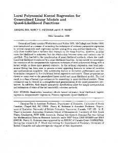
Mean Var. HT m1 12 3085.6 22 5394.8 32 13968.2 m2 12 339.7 22 1628.5 32 8248 m3 12 3961.2 22 5666.8 32 12350.3

Linear 95.0 1612.8 10111.5 338.1 1620.7 8413.5 555.2 2335.9 9361.2

7

CV Local lin. Opt. Local lin. 96.7 (0.77) 94.4 1663.6 (0.75) 1611.8 10408.5(0.74) 10129.5 106.2 (0.21) 104.6 1516.1 (0.39) 1496.8 8599.8 (0.61) 8415.2 222.1 (0.06) 198.2 2179.1 (0.19) 1999.5 9086.2 (0.57) 8782.3

TABLE 1. Empirical design MSE of Horvitz-Thompson (HT), linear regression and local linear regression estimators. The numbers in parentheses are the average bandwidths.

5 Simulation Results In this section, we report on simulation experiments comparing the performance of the local linear regression estimator with the Horvitz-Thompson estimator given in (1) and the linear regression estimator which assumes model (3) for the population. More extensive simulations are reported in Breidt and Opsomer (1999, 1999b). The following mean functions are used: m1 (x) = 1 + 2(x ? 0:5) m2 (x) = 1 + 2(x ? 0:5)2 m3 (x) = 1 + 2(x ? 0:5) + exp(?200(x ? 0:5)2); with x 2 [0; 1]. For m1 , the linear regression estimator is expected to be competitive with the local linear regression estimator, since the assumed model is correctly speci ed. The population xi are uniformly distributed over their range. The population values yi are generated from these mean functions by adding normally distributed, independent errors. We evaluate three values for the standard deviation of the errors: 1 = 0:1; 2 = 0:4; 3 = 1. The population is of size N = 1; 000 and the sample size is n = 100. For each combination of mean function and variance, 100 replicate samples are selected. As the population is kept xed during these 100 replicates, we are able to evaluate the design-averaged performance of the estimators. Table 1 shows the mean squared error results. In all these simulations, the regression estimators perform better than the Horvitz-Thompson estimator, regardless of whether the underlying model is correctly speci ed or not, but that eect decreases as the true model variance increases. The traditional regression estimator and the local linear estimator achieve similar MSEs when the underlying function is linear. When the underlying

8

Local Polynomial Regression Estimators

function is not linear, the local linear estimator tends to achieve a smaller MSE than the traditional linear regression. That eect decreases as the model variance increases. The cross-validated MSE is larger than the design optimal MSE, but only by a small amount. Overall, the selected bandwidth adapts to the shape of the underlying mean function, as shown by the fact that the average CV bandwidths dier dramatically among the three mean functions.

References Breidt, F.J. and Opsomer, J.D. (1999). Local polynomial regression estimation in survey sampling. Working paper, Iowa State University Department of Statistics. Breidt, F.J. and Opsomer, J.D. (1999b). Implementing the local polynomial regression estimators. Working paper, Iowa State University Department of Statistics. Chambers, R.L., Dorfman, A.H. and Wehrly, T.E. (1993). Bias robust estimation in nite populations using nonparametric calibration. Journal of the American Statistical Association 88, 268{277. Cleveland, W.S. (1979). Robust locally weighted regression and smoothing scatterplots. Journal of the American Statistical Association 74, 829{ 836. Dorfman, A.H. (1992). Nonparametric regression for estimating totals in nite populations. Proceedings of the Section on Survey Research Methods, American Statistical Association, 622{625. Dorfman, A.H. and Hall, P. (1993). Estimators of the nite population distribution function using nonparametric regression. Annals of Statistics 21, 1452{1475. Fan, J. (1992). Design-adaptive nonparametric regression. Journal of the American Statistical Association 87, 998{1004. Fan, J. (1993). Local linear regression smoothers and their minimax eciencies. Annals of Statistics 21, 196{216. Horvitz, D.G. and D.J. Thompson. (1952). A generalization of sampling without replacement from a nite universe. Journal of the American Statistical Association 47, 663{685. Kuo, L. (1988). Classical and prediction approaches to estimating distribution functions from survey data. Proceedings of the Section on Survey Research Methods, American Statistical Association, 280{285. Ruppert, D., and Wand, M.P. (1994). Multivariate locally weighted least squares regression. Annals of Statistics 22, 1346{1370. Sarndal, C.-E., Swensson, B., and Wretman, J. (1992). Model Assisted Survey Sampling, Springer, New York.