The Approximate Option Pricing Model: Performances and Dynamic ...

The Approximate Option Pricing Model: Performances and Dynamic Properties¤ Gunther Capelle-Blancardy

Emmanuel Jurczenkoz

Bertrand Mailletx

January 2001

Abstract Using high frequency data from ParisBourse SA, this article examines pricing and hedging performances of the Jarrow and Rudd (1982) model. We …rst …nd that this model improves the pricing of CAC 40 index European call options whether in-sample or out-of-sample, and whatever economic or statistic criterion may be used. Moreover, simple models for implied moments lead - in a dynamic setting - to results very close to those from in-sample optimization. But, we also …nd that this model does not improve hedging strategy and that the Black and Scholes (1973) model is still di¢cult to beat. Keywords: Option Pricing Models, Volatility, Skewness, Kurtosis. JEL Classi…cation: G.10, G.12, G.13.

We thank Bernard Bensaïd, Thierry Chauveau, Charles Corrado, Eric Jondeau, Ike Mathur (the referee), Thierry Michel, Fariborz Moshirian (the editor), Christophe Villa for their comments and suggestions. We also gratefully acknowledge comments by participants at the VIIth International Conference in Forecasting Financial Markets (London, May 2000), the XVIIth “Journées de Microéconomie Appliquée” (Québec, June 2000), the XVIIth International Meeting of the GDR-CNRS Money and Finance (Lisbon, June 2000), the XVIIth AFFI International Conference in Finance (Paris, June 2000), the IXth European Financial Management Association Meetings (Athens, July 2000), the IVth International Congress on Insurance, Mathematics and Economics (Barcelona, July 2000), the ILth Conference of AFSE (Paris, September 2000), the XIIIth Australasian Finance and Banking Conference (Sydney, December 2000). The usual disclaimers apply. y TEAM-CNRS - University of Paris I Panthéon-Sorbonne. 106-112 Bd de l’Hôpital 75647 Paris Cedex 13 FRANCE. Tel: (33 1) 44 07 82 71/70 (facsimile). E-mail: [email protected]. z TEAM-CNRS - University of Paris I Panthéon-Sorbonne. E-mail: [email protected]. x TEAM-CNRS - University of Paris I Panthéon-Sorbonne, ESCP and A.A.Advisors (ABNAMRO Group). E-mail: [email protected]. ¤

1

1. Introduction Several papers reports that the Black-Scholes (1973) model is somehow inconsistent with stylized facts since it misprices out-of-the-money and in-the-money options (see Bates, 1996, for a review). This result is partially attributed to the underlying asset return log-normality hypothesis and di¤erent processes have been considered.1 But these approaches focusing on …nding the “right” distribution, which are not parsimonious, could lead to some estimation problems, and, as shown by Das and Sundaram (1999), could imply a volatility term structure di¤erent from the observed one. An alternative technique consists in using binomial or trinomial lattices (see Rubinstein, 1994, for instance) that achieve an exact cross-sectional …t of option prices. Nevertheless, over…tting and variability of the volatility through time, which is supposed to be a deterministic function of asset price, maturity and moneyness, are potential shortcomings of pricing with trees (see Dumas et al., 1998). Another approach, originally developed by Jarrow and Rudd (1982), consists in approximating the underlying return density with a normal or a log-normal one, corrected by introducing skewness and kurtosis parameters. These models are, in some way, simpler since they require very slight additional assumptions 1

For instance, recently Bakshi et al. (1997) develop an option pricing model that admits stochastic volatility, stochastic interest rate and random jumps.

and the number of required parameters is quite small. Moreover, they seems more adapted to the estimation of risk-neutral density. The aim of this article is to check whether the approximation proposed by Jarrow and Rudd (1982) allows to improve the pricing of CAC 40 index options traded at the MONEP (Marché des Options Négociables de Paris). First, we evaluate in-sample, out-of-sample and dynamic pricing performances using several statistic and economic criteria. Second, we compare continuous and discrete hedging performances of option pricing models under review. The paper is organized as follows. Section 2 is devoted to a short presentation of the Jarrow and Rudd (1982) model. Section 3 brie‡y describes the French option market database and the methodology. Section 4 presents empirical results on pricing and hedging performances. Section 5 concludes.

2. The Pricing of Options when Densities are Skewed and Leptokurtic Whilst Black and Scholes (1973) (hereafter BS) suppose that underlying asset returns are normally distributed, Jarrow and Rudd (1982) (hereafter JR) propose a method to price options when densities are skewed and leptokurtic. The basic idea is to approximate the unknown real density function by using deviations from

2

Gaussian moments.2 Following JR, Corrado and Su (1996) show that the price of a call option (CJR ) can be written as a function of the BS price (CBS ) as follows:

CJR (St ; K; ¿ ; rj¾; ° 1 ; ° 2 ) = CBS (St ; K; ¿ ; rj¾) + ¸1 Q3 + ¸2 Q4 8 > > < ¸1 = ° 1 (F ) ¡ ° 1 (A)

(1)

8 ³ ´3=2 ¡r¿ > da(K) > e < Q3 = ¡ (St er¿ )3 e¾2 ¿ ¡ 1 3! dSt with and ³ ´ 2 > > 2 > > : ¸2 = ° 2 (F ) ¡ ° 2 (A) : Q4 = (St er¿ )4 e¾2 ¿ ¡ 1 e¡r¿ d a(K) 4! dS 2 t

where F and A are, respectively, the “true” cumulative density function of the underlying asset price and the approximating one,° 1 (:) and ° 2 (:) are Fisher pa3=2

rameters for skewness and kurtosis that is ° 1 (:) = ¹3 (:) =¹2 (:) and ° 2 (:) = ¹4 (:) =¹22 (:) ¡ 3 with ¹i (:) the centered moment of order i, i = [2; 3; 4]. According to Jarrow and Rudd (1983) and Corrado and Su (1996), this model improves the pricing of European options. The aim of the next section is to provide an evaluation of pricing and hedging empirical performances of such a model on the French market. 2

Amongst the most used statistical series in …nance, one can distinguish expansions based on a normal distribution as Gram-Charlier Type A series (Backus et al., 1997, Corrado and Su, 1997, Knigth and Satchell, 1997, Brown and Robinson, 1999) or expansions based on Hermite polynomials (Madan and Milne, 1994, Abken et al. 1996, Jondeau and Rockinger, 1998, Ané, 1999), and Generalized Edgeworth - or Gram-Charlier - series expansion based on a lognormal distribution (Jarrow and Rudd, 1982, Corrado and Su, 1996, Jondeau and Rockinger, 1998). For a review on statistical series expansion, see Johnson et al. (1994) or Kendall and Stuart (1977).

3

3. The Data and the Estimation Procedure Our study focuses on long term European CAC 40 index call options (PXL contracts) traded at the MONEP in 1997 and 1998.3 Option series are extracted from the ParisBourse SA database which includes a time-stamped record of every trade occurred on the MONEP as well as dividends relative to underlying assets. It also contains the CAC 40 index caught every 30 seconds. The PIBOR 3 months serves as a proxy for the riskless interest rate and is obtained from Datastream T M . We adjusted the index for discrete dividends as Harvey and Whaley (1992). Because of liquidity problems, we used exclusion criteria to remove uninformative options record from the database. On the sample, more than 12,500 prices are reported. In implementing each model, we use all call options available on each given day, regardless of moneyness, as inputs for estimating implied parameters.4 In backing out implied parameters from all option prices on a day, we allow parameters to vary from day to day, which is inconsistent with the models assumption if parameters proved to be truly variable. Therefore, this procedure su¤ers from a main, but usual, shortcoming. However, as noted by Renault (1997), even though there are 3

For more details about the database, see Capelle-Blancard et al. (2001). We use the Broyden, Fletcher, Goldfarb and Shanno (BFGS) optimization algorithm. Despite the widespread use of option-implied volatilities, there is no general agreement regarding weighting scheme (see Bates, 1996). We adopt the simplest strategy using the same weight for all options, since, anyway, our main goal is to provide equal chance to both models. Moreover, Corrado and Miller (1996) shown that simultaneous equations estimators and weighted average estimators have the same attainable variance lower bound, and, therefore, are equally e¢cient when used with appropriate weights. Additionnally, we check the sensitivity of the parameter estimations in several ways and report similar results. See Capelle-Blancard et al. (2001). 4

4

no theoretical foundation for such a practice, it provides a quick and relatively accurate pricing strategy. Moreover, most empirical studies use this procedure (see, for instance, Bakshi et al., 1997 and Dumas et al., 1998).5

4. Empirical Results on CAC 40 Index Options In the next sub-section, we present in-sample and out-of-sample results and document simple dynamic properties of models performances. Then, we turn in the following sub-section to measure the improvement obtained when pricing models are applied to hedging strategies.

4.1. The Alternative Models Pricing Performances We computed several criteria in order to get the di¤erent aspects of the di¤erences between the two model pricing errors: the Mean Error, the Mean Absolute Error, the Mean Absolute Percentage Error, the Root Mean Square Error, the Standard Deviation of Error (expressed here in FRF), the Percentage of Positive Error, and the Overestimation and the Underestimation frequency at a 5% threshold. As pointed by Leitch and Tanner (1991) and Satchell and Timmerman (1995), 5

Capelle-Blancard et al. (2001) shows that volatilities obtained with the two models are relatively similar (varying between 17% and 30 % with a correlation coe¢cient equal to 0.8951). Not surprisingly, on the whole sample, the implied distribution seems to be asymmetric since the skewness is negative. The implied distribution seems to be leptokurtic since the kurtosis is higher than three in general. Moreover, those parameters seems to exhibit strong autoregressive characteristic.

5

goodness-of-…t is not the only criterion to consider. That is the reason why the comparison also relies on fourth other economic criteria. First, we assume a logarithmic utility function and compute the Mean Logarithmic Error, which results in a logarithmic transformation of the error terms. Second, we document two asymmetric loss functions: the Mean Mixed Error for Underestimations, which overweights the underestimation errors adopting the seller’s point of view who prefers to sell at an higher price than the market price and the Mean Mixed Error for Overestimation, which symmetrically, puts more weight on the overestimation errors, stressing the buyer’s point of view who prefers to buy at a lower price than the market price.6 Last, following Hwang and Satchell (1998) and Hwang et al. (1999), we advocated the use of the Cumulative Linex loss function.7 In Table 1 are reproduced pricing performances according to several criteria. First, the comparison between BS and JR models leads in general to the conclusion of a better …t of the second model. BS mean absolute error is equal to FRF 5.30 (which represents a mean relative error of 10.18% when considering option prices) to be compared with 2.17 (3.55%) for JR. Furthermore, the two models 6

See Capelle-Blancard et al. (2001) for complete de…nitions. Cumulative Linex as: ¡ £ ¡ is¤de…ned ¢¤ ¢ ¤ P loss£ function ¤ obs CLinex (CN )= N exp ¡a C ¡ C + a Cn¤ ¡ Cnobs ¡ 1 where Cn¤ is the theoretn n n=1 ical price, Cnobs the market price at time n and a an arbitrary coe¢cient as a function of the sensitivity of the representative agent to pricing error. Indeed, with an appropriate Linex parameter, we can re‡ect small (large) losses for underestimation or overestimation. In particular, a positive a will re‡ect small losses for overestimations comparatively to large losses for underestimations. 7

6

Table 1: Pricing performances Black and Scholes

Jarrow and Rudd

In-sample

All sample

OTM

ATM

ITM

All sample

OTM

ATM

ITM

ME (FRF) MAE (FRF) MAPE RMSE (FRF) STD (FRF) PPE UPE (5%) OPE (5%) MLNE (FRF) MME(U) MME(O) CLINEX (a = 0:1)

-0.61 5.30 10.18 0.07 8.11 56.04 8.15 39.56 0.06 53.48 18.08 4.4£1012

4.71 4.93 21.44 0.09 3.79 95.32 1.42 84.34 0.17 6.99 34.57 4,855

-0.83 3.95 5.44 0.07 5.41 50.35 11.30 24.65 0.02 24.16 9.92 1,444

-9.41 9.52 2.88 0.30 11.17 1.90 11.70 0.04 -0.03 212.42 10.54 4.4£1012

-0.14 2.17 3.55 0.04 4.83 50.17 9.74 10.00 -0.00 17.64 8.02 4.3£1010

0.04 1.53 6.37 0.04 2.65 50.57 21.78 20.11 -0.01 4.80 3.92 3,780

-0.07 2.04 2.63 0.04 2.95 50.80 5.21 6.90 0.00 5.77 5.11 295

-0.64 3.63 0.99 0.20 9.50 47.81 0.51 0.38 0.00 71.47 22.88 4.3£1010

AIC BIC SIC AICc

23,104 23,110 21,106 5.18

17,386 17,402 17,392 4.15

Out–of-sample ME (FRF) MAE (FRF) MAPE RMSE (FRF) STD (FRF) PPE UPE (5%) OPE (5%) MLNE (FRF) MME(U) MME(O) CLINEX (a = 0:1)

-1.10 6.29 11.31 0.09 9.41 50.19 16.30 36.29 0.05 68.71 27.40 4.9£1012

3.97 5.51 22.47 0.11 6.35 79.27 13.42 68.69 0.14 12.08 49.62 3,864

-1.20 5.45 7.08 0.10 7.60 49.02 19.44 28.58 0.02 45.85 18.95 4,086

-9.71 9.85 2.98 0.31 11.58 2.56 13.06 0.08 -0.03 227.48 10.89 4.9£1012

-0.62 4.29 7.63 0.07 7.48 45.74 22.46 17.93 -0.02 38.88 21.80 2.8£1012

-0.82 3.96 14.99 0.09 5.92 42.74 44.02 28.29 -0.07 23.30 16.51 5,756

-0.34 4.22 5.12 0.08 6.38 48.99 16.37 17.28 0.00 25.69 19.48 1,847

-0.98 5.02 1.39 0.24 11.48 42.44 0.89 1.57 -0.00 100.69 37.11 2.8£1012

Table 1 reports the mean error, the mean absolute error, the mean absolute percentage error, the root mean square error, the mean logarithmic error, the standard deviation of error, the percentage of positive error, the overestimation and the underestimation frequency (at a 5% threshold), two mean mixed error statistics and the Cumulative Linex, as well as di¤erent information criteria: AIC, AICc, BIC, and SIC. In panel A, implied parameters have been backed out, each day, by minimizing the sum of squared errors for all call option prices available on that day if the number of transactions was equal or greater than 25, or on that day and previous days if the number of transactions was lower than 25. In panel B, implied parameters have been backed out, each day, by minimizing the sum of squared errors for all call option prices available the days before. Letters OTM, ATM and ITM stand, respectively, for out-of-the-money, at-the-money and in-the-money options. The sample period extends from Jan. 2, 1997 through Dec. 30, 1998.

have a slight tendency to underprice options since the mean error is negative for all of them, but this mean underpricing is lower for the JR model. The root mean squared error and the error standard deviation are also drastically reduced. Moreover, whilst the BS model goes with large overpricing at a large frequency (more than the third of the error sample - 39.56% - corresponds to large positive error), the JR model gives better results: the percentage of positive error is approximately equal to 50% and the frequency of large errors (positive or negative) are similar and equal to 10% or so. Moreover, whatever the point of view adopted, a seller or a buyer of options would prefer the JR model since the mean logarithm error, the mean mixed errors for overpricing and for underpricing are far lower with this model. The use of cumulative linex function lead to the same conclusion.8 Besides, BS model seems not adapted to price ITM and OTM options. The di¤erence between models are the strongest in relative (absolute) terms when OTM (ITM) options are considered whilst distinguishing options according to their moneyness seems to be less relevant when JR model is estimated.9 Figure 1, which represents a non-parametric estimation of the density of the in-sample 8

It is also interesting to note that both skewness and kurtosis lead to improve the pricing performances but the skewness adjustment gives better results than the kurtosis adjustment. See Capelle-Blancard et al. (2001) for a comparison between JR model with skewness adjustment but without kurtosis adjustment and the JR model with kurtosis adjustment but without skewness adjustment. 9 On the contrary, the e¤ect of time to maturity is less evident. One could have expected to …nd a greater di¤erence between models when maturities are long. But, as in Backus et al. (1997), such relation is not valid in our sample.

8

errors, con…rms those results.10

Fig 1: Density of in-sample errors. The solid (dotted) line corresponds to JR (BS).

Improvements obtained are quite not surprising since we have supplementary degrees of freedom to improve the goodness-of-…t. Information criteria, such as Akaïke Information Criterion (AIC), Corrected Akaïke Information Criterion (AICc), Bayesian Information Criterion (BIC), or Schwartz Information Criterion (SIC), based on in-sample performances are also reported. Those are computed to examine the possibility of over…tting as they penalize the presence of more parameters. On the basis of those criteria, JR model dominates BS one. Finally, considering out-of-sample pricing performance all statistic and economic criteria are reduced by far when JR model is used and this positive result holds whatever 10

A non parametric kernel density estimator was used with Silverman’s rule of thumb.

9

the moneyness. For instance, the BS model mean absolute error is equal to FRF 6.29 (11.31%) while the JR model mean absolute error is equal to FRF 4.29 (7.63%).11 We can also remark that JR out-of-sample error dominates the BS one according to the second (and …rst) order dominance criterion since the probability of a smaller error (in absolute terms) is always higher in the JR model.

4.2. The Alternative Models Dynamic Performances When adopting a dynamic approach, the problem of recovering the true expected option prices is more tricky - as underlined by Vénutelio and Péllieux (1997) and several methods have been already proposed. The …rst approach relies on numerical methods based on Monte-Carlo simulations (see Scott, 1987) but it is time and computational consuming. The second approach consists in providing a closed-form solution using hypotheses on the distribution of the asset returns and on the structure of moments variations. For instance Heston and Nandy (1997) give an approximation of the fair price of an option when the underlying process conforms to a GARCH(1,1)-M model. Some distributional assumptions in particular the normality of conditional returns - are nevertheless required. The third way of dealing with a dynamic framework is to suppose - as Hull and White 11

These results obtained with the BS model on the MONEP are not as accurate as those reported from the CBOE by Corrado and Su (1996), Bakshi et al. (1997) or Dumas et al. (1998). For instance, the BS mean absolute error reported by Corrado and Su (1996) is equal to USD 0.875 (about 4.3%).

10

(1987) - that one can have a good approximation of the fair price of an option by expanding the traditional BS formula around the expected implicit parameter values.12 Adapted to our general valuation problem, this approach - considering a …rst order approximation - leads to the following price of a call denoted C(t):

C(t) » = C [E (£t )] +

±C [E (£t )] [£t ¡ E (£t )] ±£t

(2)

where either £t = ¾ t or £t = (¾ t ; ° 1t ; ° 2t ) when BS or JR model is considered: In this case, another problem has to be solved: the choice of the conditional moments model involved in the option pricing relations. A generalization of the previous approach can be attempted by considering a density function L (:) - which has not to be precisely de…ned providing its relative …rst four moments exist - whose each conditional moment has an autoregressive structure.13 We consider two di¤erent ways of modeling conditional moments. The …rst approach considers a martingale for conditional moments; in such a case, the 12

This approach, as pointed by Dumas et al. (1998), is supposed to be inferior because it is not consistent to use BS option pricing model when the volatility varies through time. Nevertheless, two arguments support this approach. If the implied parameters involved in the pricing of option does not vary too much, we should obtain a good approximation, and this could be the best way of explaining market practises. 13 Because of the “smile” problem, several authors have also proposed to substitute the volatility parameter by a volatility function which is consistent with the empirical moneyness and maturity biases. Among these authors, Dumas et al. (1998) proposed a Deterministic Volatility Function (DVF) depending on maturity and strike. Unfortunately, this kind of deterministic function have been found to exhibit time instability and this approach performs poorly when using such a deterministic function because the estimated volatility change substantially through time.

11

best predictor of future conditional moments would be the unconditional ones. This assumption implies the following setting when considering a general model implying the …rst four moments: E(¹it ) = ¹it¡1 for t = [1; 2; :::; T ] where ¹it ; i = [1; 2; 3; 4] ; are the …rst four conditional moments relative to the general density L (:). This updated option pricing model, which can be de…ned as a benchmark, uses implied moments as proxies of the moments of the index return density, as already done previously. The second model consist in estimating the best predictor of conditional moments.14 In such a case, the best predictor of future conditional moments would be written E(¹it ) = ®0it + ®1it ¹it¡1 + ®2it ¹it¡2 for t = [1; 2; :::; T ] where ¹it ; i = [1; 2; 3; 4] , are the …rst four conditional moments relative to the general density L (:) and ®0it ; ®1it ,®2it are parameters obtained by rolling regressions. The optimal theoretical prices are based on the assumption that we can model implicit conditional moments through an AR(2) process.15 Then, prices are computed using expected implied moments plugged into the Hull and White’s approximation. 14

Lots of literature has already been dedicated to model conditional moments and the most popular is certainly the GARCH model family developed by Engle (1982) and Bollerslev (1986). In addition, previous works have already reported a signi…cant autoregressive characteristic of skewness of asset return density. Sangupta and Park (1990) and Sangupta and Zheng (1997), the former working on the US stock market and the latter on a US mutual fund database, use this kind of models and conclude to the signi…cance of the valuation of higher moments than the …rst two by the market participants. 15 The choice of an AR(2) was done on an arbitrary basis according to the results of Sangupta and Park (1990) and Sangupta and Zheng (1997). Such criteria as AIC, BIC, AICc and SIC lead to an higher order model. Nevertheless, practical considerations make us to consider a simpler model.

12

Table 2 reports the results of the comparison of the two sets of models. In this section, we adopt the point of view of an operator who, with respect to all the available information, would price a speci…c option. For this purpose, we construct a new sample, with the original database, in which we have, every …fteen minutes, the price of the index, the price of an option of a speci…c maturity and the proxy of the riskless interest rate. With this …ltered data composed of regularly spaced series, we then compute - through the optimization procedures described previously - the implied parameters using all options in the last twenty four hours (i.e. corresponding to rolling twenty-four hours optimization windows). In comparison with the previous methodology where the optimization was conducted in the current business day, this allows to take into account potential severe changes in the market. The result of the comparison between both models under evaluation leads, once again, to conclude to the superiority of the JR model. Indeed, when Random Walk and AR(2) hypotheses for implied parameters are adopted, most of the criteria are drastically reduced for the more general model. Moreover, in the AR(2) case, the results obtained in this section are very close to those corresponding to the in-sample estimation (see Table 1). All comparisons allow to conclude to the superiority of the JR model for all the selected criteria, but one question remains: is this improvement su¢cient to make a di¤erence in term of hedging performance?

13

Table 2: Dynamic comparison

ME (FRF) MAE (FRF) MAPE RMSE (FRF) STD (FRF) PPE UPE (5%) OPE (5%) MLNE (FRF) MME(U) MME(O) CLinex (a = 0:1)

Random Walk

AR (2)

Black-Scholes Jarrow-Rudd

Black-Scholes Jarrow-Rudd

-1.05 6.26 11.03 0.16 11.79 51.30 13.40 36.55 0.05 20.93 6.38 184

-0.43 3.63 6.27 0.11 8.13 48.41 17.96 16.57 -0.02 36.35 7.73 316

-1.82 4.03 6.44 0.14 4.56 41.91 6.60 27.87 0.03 21.50 6.69 189

-0.64 2.13 3.18 0.08 2.88 40.59 8.56 7.01 0.00 6.94 4.03 61

Table 2 reports the mean error, the mean absolute error, the mean absolute percentage error, the root mean square error, the mean logarithmic error, the standard deviation of error, the percentage of positive error, the overestimation and the underestimation frequency (at a 5% threshold), two mean mixed error statistics and the Cumulative Linex. Implied parameters have been backed out by minimizing the sum of squared errors for all call option prices available on the last 24 hours (i.e. corresponding to rolling 24 hours optimization windows). The sample period extends from Jan. 2, 1997 through Dec. 30, 1998.

4.3. The Alternative Models Hedging Performances The aim of this sub-section is to know whether the JR model provide better risk management. This comparison is made in two steps. Indeed, two aspects should be considered when judging hedging performances: the pure model performance - via the computation of the performance of a hedge portfolio continuously rebalanced through time - and the improvement in risk management the model entails

14

- which can be measured considering the results of a traditional self-…nanced single instrument strategy discretely rebalanced. The latter takes into account realistic constraints (such as costs of strategies, discreteness of the series, tick size problems,...) whilst the former focuses only on the accuracy of the sensitivity parameters of pricing formula. We then evaluate two types of ex post hedge portfolio errors: a continuous hedge portfolio error - denoted "0t+1 - and a discrete 00

hedge portfolio error - denoted "t+1 . In the continuous case, the hedge portfolio is formed to replicate the value of an option at the next period. Following Dumas et al. (1998), we can de…ne the ex post continuous hedge portfolio error as:

"0t+1

£ obs ¤ = Ct+1 ¡ Ctobs ¡

Z

t+1

¢ (Su ; u) dSu

(3)

u=t

where ¢ (:; :) is the sensitivity of the option price to in…nitesimal variations of the underlying asset price.16 It can be shown that to a large extent the hedging replication error re‡ects the di¤erence between the two periods. Indeed, if a model determine correctly ¢ (Su ; u), and if the variation of the index price is the only relevant variable, a minimum requirement consists in the following equality: ¡ ¢ E "0t+1 = 0. If we measure prices at di¤erent time t, the ex post continuous 16

By de…nition, it is the …rst partial derivative of the option price ³with´respect to³ the´ underlying asset price, so in the case of the JR model: ¢JR = N (d) + ¸1 S3T Q3 + ¸2 S4T Q4 :

15

hedge portfolio error can be written as: ³ ´ ³ ´i £ obs ¤ h b t+1 ¡ Ct £ bt "0t+1 = Ct+1 ¡ Ctobs ¡ Ct+1 £

(4)

b t is the set of parameter required in the computation of theoretical where £

prices. The aim of this comparison of continuous hedging performances is to assess whether although the BS model exhibits pricing biases - as long as these biases remain relatively stable through time - its hedging performance is superior than the performance of a more complex model that can account for many of these biases, especially if the more complex model does not adequately characterize the way asset prices evolve over time. When we compute the improvement in continuous hedging performance con:0

0

0

0

0

sidering JR model, we have "t+1 = "JR;t+1 ¡ "BS;t+1 where "JR;t+1 and "BS;t+1 are the continuous hedging errors for BS and JR models. Taking the expectation of ³:0 ´ ¡ BS ¢ ¡ ¢ JR the last equation gives: E "t+1 = E Ct+1 ¡ Ct+1 ¡ E CtBS ¡ CtJR and the ³:0 ´ empirical counterpart of E "t+1 ; t = [1; :::; N ¡ 1] where N is the total number of observations, is:

:0

"t+1 =

´i ´ ³ 0 h³ 0 1 0 0 "JR;N ¡ "JR;1 ¡ "BS;N ¡ "BS;1 (N ¡ 1)

(5)

As pointed by Nandy and Wagonner (2000), the expected improvement in 16

hedging is related to the di¤erence between hedging error variations computed for two dates. Table 3 con…rms that the improvement is accordingly very small. All statistic and economic criteria values are very close for both models whatever the criterion considered is. In that sense, the JR model fails to improve signi…cantly continuous hedging and BS model remains a di¢cult benchmark to beat. In order to compute a discrete hedge portfolio error, we build a traditional self-…nanced single instrument strategy based upon CAC 40 index contracts. The 00

ex post hedging error, at time t + 1, denoted "t+1 , is calculated as follows:

00

"t+1 = ¢t St+1 + [Ct ¡ ¢t St ] ert ¡ Ct+1

(6)

where rt is equal to the risk-free rate for the business day t. This calculation is repeated for every t and for all options in the sample.17 When we compute the improvement in discrete hedging performance consider: 00

00

00

ing JR model, we get this time (with previous notations) "t+1 = "JR;t+1 ¡"BS;t+1 = 17

To hedge the sell of a call option at time t, the investor has to be long in ¢t shares of the underlying asset and invest the residual (i.e. Ct ¡ ¢t St ) in a risk-free bond. While the hedged portfolio is supposed to be riskless when there is an unique source of risk and when the hedging portfolio is rebalanced continuously, practical considerations - such as transaction costs or divisibility problems - lead some authors to evaluate discrete-time hedging performance where adjustments are made at discrete intervals. We suppose hereafter that the portfolio is rebalanced every business days. For examples of perfect delta-neutral hedges, see Bakshi et al. (1997).

17

£

¤ BS ¢JR [St+1 ¡ St ert ]. Taking the expectation gives: t ¡ ¢t ³ : 00 ´ ³ : ´ ³ ´ ³ : ´ E "t+1 = E ¢t E Set+1 ¡ Cov ¢t ; Set+1

(7)

:

BS with ¢t = ¢JR and Set+1 = St+1 ¡ St ert : t ¡ ¢t

The expected improvement in hedging performance depends on the product

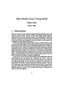
of expected di¤erence in deltas, weighted by the expected premium on the index, and the covariance between the di¤erences in deltas and ex post premia. It is then interesting to evaluate those components. First, we can notice, that the overall improvement depends crucially on the …rst term since the term in covariance is very low (it is equal to -0.0036 on the sample). Moreover, for the whole sample, the mean absolute di¤erence between deltas is, in absolute (relative) term, equal to 0.0079 (2.05%) - varying from -0.004 to 0.11 - as illustrated in Figure 3. In fact, when taking into account skewness and kurtosis, hedging coe¢cients have not been found very di¤erent one to another. In other words, since the co:

variance between ¢t and Set+1 is small, the hedging coe¢cient ¢JR is not, on our t data, enough sensitive to departures from normality for causing a major improve-

ment in discrete hedging strategies as indicated in Table 3. When focusing on discrete delta-hedge strategy performance and for BS model, the mean hedging error is equal to FRF -1.73 and the mean absolute hedging error is equal to FRF 6.58 when considering at-the-money call options (and, respectively, FRF -2.28 and 18

FRF 7.58 for the whole sample). These statistics are similar to those reported in Ané (1999) on the CBOE market since mean hedging error is USD -0.0753 and mean absolute hedging error is USD 0.5 for medium term options. Results regarding discrete hedging performances obtained with BS and JR models are very close whatever the moneyness and the maturity. Most of the criteria are roughly the same for both models.

Fig 2: Scatter-plot of deltas

Neither the importance of improvement, nor the directional accuracy criteria allows to conclude to the dominance of the JR model: the delta computed with the BS model is corrected in a right direction when taking into account skewness and kurtosis in only 44 % of the observations on the whole sample.18 18

As the sensitivity of option prices to index return is an increasing function of the strike

19

Table 3: Hedging performances Black and Scholes

Jarrow and Rudd

Continuous hedging

All sample

OTM

ATM

ITM

All sample

OTM

ATM

ITM

ME (FRF) MAE (FRF) RMSE (FRF) STD (FRF) PPE MME(U) MME(O) CLINEX (a = 0:1)

0.02 1.93 0.05 5.45 45.39 12.22 19.59 2.5£1011

0.00 1.17 0.03 1.90 43.85 2.51 2.46 72.08

0.00 1.95 0.04 3.07 46.02 5.64 5.91 285.31

0.12 3.49 0.29 12.23 46.54 53.72 99.45 2.5£1011

0.02 1.99 0.05 5.51 45.48 12.61 19.93 2.5£1011

0.00 1.20 0.03 1.97 43.96 2.68 2.59 78.39

0.00 2.03 0.04 3.22 46.15 6.14 6.41 314.38

0.13 3.51 0.29 12.25 46.54 54.18 99.64 2.5£1011

-1.73 6.58 6.21 0.63 14.09 49.60 21.23 17.46 -0.05 180.64 27.31 1.3£109

-3.70 10.41 2.21 1.59 38.14 47.74 5.55 1.73 -0.06 1,204 271.96 1.6£1020

-1.62 6.37 6.16 0.62 13.88 50.39 20.83 17.65 -0.05 175.38 26.21 1.3£109

-3.88 10.43 2.21 0.32 38.17 45.13 5.55 1.56 -0.06 1,206 274.21 1.6£1020

Discrete hedging ME (FRF) MAE (FRF) MAPE RMSE (FRF) STD (FRF) PPE UPE (5%) OPE (5%) MLNE (FRF) MME(U) MME(O) CLINEX (a = 0:1)

-2.28 7.58 9.31 0.66 25.45 50.06 19.70 18.09 -0.11 541.64 118.54 1.6£1020

-0.96 4.84 23.02 0.40 8.12 53.88 37.62 41.74 -0.28 56.09 15.64 3,727

-2.25 7.59 10.02 0.66 25.45 49.53 19.43 18.63 -0.13 540.49 119.88 1.6£1020

-0.75 5.12 25.68 0.41 8.31 54.61 37.13 43.68 -0.34 56.04 18.72 3,871

Table 3 reports the mean error, the mean absolute error, the mean absolute percentage error, the root mean square error, the mean logarithmic error, the standard deviation of error, the percentage of positive error, the overestimation and the underestimation frequency (at a 5% threshold), two mean mixed error statistics and the Cumulative Linex. Implied parameters have been backed out, each day, by minimizing the sum of squared errors for all call option prices available on that day if the number of transactions was equal or greater than 25, or on that day and previous days if the number of transactions was lower than 25. Letters OTM, ATM and ITM stand, respectively, for out-of-the-money, at-the-moneyand in-the-money options. The sample period extends from Jan. 2, 1997 through Dec. 30, 1998.

This quite negative result strongly di¤ers from those of Ané (1999) who applied Madan and Milne (1994) model on CBOE market. This failure could have di¤erent explanations. The …rst one could be found in a non signi…cative improvement of the JR model. In other words, the accuracy of the JR model is unfortunately still not su¢cient for making a real di¤erence with the BS model when it is used for hedging purposes, but this …rst hypothesis contradicts results reported in previous sections that shown an important di¤erence between models accuracy. Another explanation of this failure could merely rely on the implied parameters variability - which entails movements in deltas that are not linked with price variations as ³ : ´ hightlighted by the term Cov ¢t ; Set+1 .

5. Conclusion Our results lead to the conclusion that the Jarrow and Rudd (1982) option pricing model can, at least partially, explain the “smile” phenomenon and is superior in term of pricing errors. Both statistical and economic values attached to this model are better on the CAC 40 index option market than those relative to the Black and Scholes (1973) model. This is true in-sample - as expected - because of the addition of two supplementary parameters which helps for …tting the data; price, the relative error committed for both models naturally increases with the moneyness and the maturity of the option considered, but we …nd that the di¤erence in hedging performance between the two models does not depend on these speci…c characteristics.

21

it is also true out-of-sample. Nevertheless, the di¤erence between deltas are not important enough to yield a signi…cant improvement when hedging is the key issue of the use of options: the Black-Scholes model still remain a di¢cult benchmark to beat. These conclusions point us in a number of directions for future research. The …rst one is, following the approach of Hwang and Satchell (1998) or Rosenberg (2000), to focus on a dynamic approach of the comparison between models, using autoregressive forms of the three parameters dynamic considered in the option pricing model. Another concerns the use of di¤erent statistical series expansion. The use of a Gamma distribution (Heston, 1993) or a Beta distribution (Corrado,1999) as approximation of the true distributions constitute also interesting alternative approaches. A third direction would consist in a general comparison of the hedging performance and the pricing accuracy of the di¤erent forms of four-moment option pricing models.

22

References Abken P., D. Madan and S. Ramamurtie, (1996), “Estimation of RiskNeutral and Statistical Densities by Hermite Polynomiale Approximation with an Application to Eurodollar Futures Options”, Working Paper Federal Reserve Bank of Atlanta. Ané Th., (1999), “Pricing and Hedging S&P 500 Index Options with Hermite Polynomial Approximation: Empirical Tests of Madan and Milne’s Model”, Journal of Futures Markets 19 (7), 735-758. Backus D., S. Foresi, K. Li and L. Wu, (1997), “Accounting for Biases in Black-Scholes”, Working Paper, Stern School of Business, 40 pages. Bakshi G., Ch. Cao and Z. Chen, (1997), “Empirical Performance of Alternative Option Pricing Models”, Journal of Finance 52 (5), 2003-2049. Bates D., (1996), “Testing Option Pricing Models”, Handbook of Statistics 14: Statistical Methods in Finance, Maddala and Rao Eds, 567-611. Black F. and M. Scholes, (1973), “The Pricing of Options and Corporate Liabilities”, Journal of Political Economy, 637-655. Bollerslev T., (1986), “Generalized Autoregressive Conditional Heteroskedasticity”, Journal of Econometrics 31 (3), 307-327. Brown C. and D. Robinson, (1999),“Option Pricing and Higher Moments”, Proceedings of the 10th annual Asia-Paci…c Research Symposium, February, 36 pages. Capelle-Blancard G., E. Jurczenko and B. Maillet, (2001), “The Approximate Option Pricing Model: Empirical Performances on the French Market”, Cahiers de la MSE, January, 54 pages. Corrado Ch., (1999),“General Purpose, Semi-Parametric Option Pricing Formulas”, Working paper of Department of Finance, University of MissouriColumbia, 36 pages. Corrado Ch. and T. Miller, (1996), “E¢cient Option-Implied Volatility Estimators”, Journal of Futures Markets 16 (3), 247-272. Corrado Ch. and T. Su, (1996), “S&P 500 Index Option Tests of Jarrow and Rudd’s Approximate Option Valuation Formula”, Journal of Futures Markets 16 (6), 611-629. Corrado Ch. and T. Su, (1997), “Implied Volatility Skews and Stock Index Skewness and Kurtosis Implied by S&P 500 Index Option Prices”, Journal of Derivatives, summer. Das S. and R. Sundaram, (1999), “Of Smiles and Smirks: A TermStructure Perspective”, Journal of Financial and Quantitative Analysis 34 23

(2), 211-240. Dumas B., J. Fleming and R. Whaley, (1998), “Implied Volatility Functions: Empirical Tests”, Journal of Finance 53 (6), 2059-2106. Dupire B., (1998), “Pricing and Hedging with Smiles”, Volatility New Estimation Techniques for Pricing Derivatives, R. Jarrow (Ed.), Risk Books. Engle R., (1982), “Autoregressive Conditional Heteroscedasticity with Estimates of the Variance of United-Kingdom In‡ation”, Econometrica 50 (4), 987-1007. Harvey C. and R. Whaley, (1992), “Dividends and S&P 100 Index Option Valuation”, Journal of Futures Markets 12 (2), 123-137. Heston S., (1993), “Invisible Parameters in Option Prices”, Journal of Finance, 48(3), 933-947. Heston S. and S. Nandi, (1997), “A Closed-Form GARCH Option Pricing Model”, Federal Reserve Bank of Atlanta Economic Review, Working Paper, November. Hull J. and A. White, (1987), “The Pricing of Option with Stochastic Volatilities”, Journal of Finance 42, 281-300. Hwang S., J. Knight and S. Satchell, (1999), “Forecasting Volatility Using LINEX Loss Functions”, manuscript, Trinity College, University of Cambridge, 20 pages. Hwang S. and S. Satchell, (1998), “Implied Volatility Forecasting: A Comparison of Di¤erent Procedures Including Fractionally Integrated Models with Applications to UK Equity Options”, in Forecasting Volatility in the Financial Markets, Knight and Satchell Eds (BH), 193-225. Jarrow R. and A. Rudd, (1982), “Approximate Option Valuation for Arbitrary Stochastic Processes”, Journal of Financial Economics 10, 347-369. Jarrow R. and A. Rudd, (1983), “Tests of an Approximate Option Valuation Formula”, in Option Pricing Theory and Applications, Brener Ed., Lexington MA: Lexington Books, 81-100. Jondeau E. and M. Rockinger, (1998), “Reading the Smile: The Message Conveyed by Methods which Infer Risk Neutral Density”, CEPR Discussion Paper 2009. Johnson N., S. Kotz and N. Balakrishnan, (1994), Continuous Univariate Distributions, Second Edition, Vol. 1, John Wiley, New-York. Kendall M. and A. Stuart, (1977), The Advanced Theory of Statistics, Fourth Edition, Vol. 1, Macmillan Publishing Company, New York. Knight J. and S. Satchell, (1997), “Pricing Derivatives Written on Assets with Arbitrary Skewness and Kurtosis”, manuscript, Trinity College, 24

University of Cambridge. Leitch G. and J. Tanner, (1991), “Economic Forecast Evaluation: Pro…t versus the Conventional Error Measures”, American Economic Review 81 (3), 215-231. Madan D. and F. Milne, (1994), “Contingent Claims Valued and Hedged by Pricing and Investing in a Basis”, Mathematical Finance 4, 223-245. Nandy S. and D. Wagonner, (2000), “Issues in Hedging Options Positions”, Federal Reserve Bank of Atlanta Economic Review, First Quarter 2000, 24-39. Renault E., (1997), “Econometric Models of Option Pricing Errors, Advances in Economics and Econometrics: Theory and Applications 3, Kreps and Wallis Eds., ESM, Cambridge University Press, 221-278. Rosenberg J., (2000), “Implied Volatility Functions: A Reprise”, Journal of Derivatives 51, Spring 2000, 51-64. Rubinstein M., (1994), “Implied Binomial Trees”, Journal of Finance 49, 771-818. Sangupta J. and H. Park, (1990), “Portfolio E¢ciency Tests based on Stochastic Dominance and Cointegration”, Working Paper in Economics #890, University of California, Santa Barbara. Sangupta J. and Y. Zheng, (1997),“Estimating Skewness Persistence in Market Returns”, Applied Financial Economics 7, 559-566: Satchell S. and A. Timmermann, (1995), “An Assessment of the Economic Value of Non-linear Foreign Exchange Rate Forecasts”, Journal of Forecasting 14, 477-497. Scott L., (1987), “Option Pricing When the Variance Changes Randomly: Theory, Estimators and Applications”, Journal of Financial and Quantitative Analysis 22, 419-438. Stein E. and J. Stein, (1991), “Stock Price Distributions with Stochastic Volatility”, Review of Financial Studies 4, 727-752. Venutolo T. and G. Péllieux, (1997), “Empirical Results from the GARCH Option Pricing Model”, Proceedings of the AEA-BNP-Imperial College Conference, June, 28 pages.

25