The Aquarius Salinity Retrieval Algorithm Recent Progress and Remaining Challenges T. Meissner, F. Wentz, L. Ricciardulli, K. Hilburn, J. Scott Remote Sensing Systems Santa Rosa, California, USA
[email protected] Abstract — This paper summarizes the major steps of the updates in the Aquarius Level 2 ocean surface salinity (SSS) retrieval from Version 2.0 to Version 3.0, which is scheduled to be released in May 2014. We first discuss the algorithm improvements in the surface roughness correction, which also includes a retrieval of wind speeds from combined Aquarius radiometer – scatterometer measurements, improvements in the correction for the reflected galactic radiation, and masking of undetected RFI. We then present a validation study for the new salinity product, which consists in an intercomparison between Aquarius, in-situ buoy salinity measurements from the ARGO network, moored PMEL buoys and the HYCOM model salinity field. Keywords — Ocean Surface Salinity; L-band microwave radiometers; L-band wind speeds; Aquarius.
I.
Fig 1. Probability density function (PDF) of Aquarius wind speeds from the scatterometer HH-pol (left) and combined scatterometer HH-pol / radiometer H-pol (right) compared to collocated RSS V7 WindSat wind speeds. The time colocation window is 120 min.
BACKGROUND
The Aquarius L-band radiometer/scatterometer system is designed to provide ocean surface salinity at an accuracy of 0.2 psu for monthly 150 km averages [1]. This poses a challenge for the instrument design and calibration as much as for the salinity retrieval algorithm [2]. Many sizeable spurious signals have to be removed to a high level of accuracy. II.
SURFACE ROUGHNESS CORRECTION
The correction for the roughness of the ocean surface in Aquarius V2.0 was based on auxiliary wind speed field from NCEP GDAS. The surface roughness correction in V3.0 uses wind speeds that are derived from combined Aquarius radiometer and scatterometer [3] observations. The details of the Aquarius wind speed retrieval algorithm and its application to the surface roughness correction are given in [4], [5]. As shown there, the use of scatterometer measurements wind speeds improves the accuracy of the surface roughness correction significantly. III.
Fig. 2. Probability density function (PDF) of Aquarius wind speeds from the scatterometer HH-pol (left) and combined scatterometer HH-pol / radiometer H-pol (right) compared to collocated buoy wind speeds. The time colocation window is 60 min.
The results of the triple colocation of Aquarius – WindSat – Buoy wind speeds are given in TABLE I and TABLE II. TABLE I. STANDARD DEVIATIONS (M/S) FOR TRIPLE COLOCATIONS OF AQUARIUS COMBINED SCATTEROMETER (HH-POL) / RADIOMETER (H-POL) WIND RETRIEVALS WITH WINDSAT AND BUOYS.
AQUARIUS WIND SPEEDS
The Aquarius L-band combined scatterometer and radiometer wind speeds, which are used as input to the surface roughness correction, provide a stand-alone product of excellent accuracy. We have validated the Aquarius wind speed versus WindSat and buoys. Fig 1 and Fig. 2 show the PDF for rain free observations. As the Aquarius, WindSat and buoy observations are mutually independent, the triple colocation method can be applied to estimate the standard deviation of each individual measurement. This work has been funded by NASA contract # NNG04HZ29C.
Aquarius WindSat
Aquarius Buoys
WindSat Buoys
0.57
1.03
1.06
TABLE II.
ESTIMATED ERRORS (M/S) OF THE INDIVIDUAL WIND SPEED MEASUREMENTS FORM AQUARIUS, WINDSAT AND BUOYS FROM THE TRIPLE COLOCATION METHOD.
Aquarius
Buoys
WindSat
0.36
0.96
0.44
ensemble of tilted facets, from which the galactic radiation is reflected. The slope probability density function for the titled facets was assumed to be Gaussian as described in Appendix A of [2]. The reflected galactic radiation can be as high as 5 K (for the average of V-pol and H-pol), which corresponds to a signal of 10 psu in salinity.
Fig. 3. Map of wind speed differences (m/s) between Aquarius (combines scatterometer – radiometer) and WindSat for the period September 2011 – August 2013.
The results of TABLE II indicate that the accuracy of the Aquarius wind speeds matches those of WindSat and other microwave radiometers (SSM/I, TMI, AMSR) and scatteromters (QuikSCAT, ASCAT). One should keep in mind though that the resolution of the Aquarius wind speeds is about 100 km, which reflects the size of the Aquarius footprint. The resolution of the other satellite wind speeds is typically about 20 – 40 km. Fig. 3 shows the absence of significant regional biases in Aquarius when compared to WindSat. One should note that the small negative bias in N Atlantic that shows in Fig. 3 is caused by RFI in the WindSat 10.7 GHz channel and not related to Aquarius. IV.
REFLECTED GALACTIC RADIATION
A. Ascending – Descending Biases in the Aquarius V2.0 Salinity Fields
Fig. 5 shows that the residual salinity error after the GO correction exceeds 1.0 psu. That means that the GO model in V2.0 correctly removes most (about 90%) of the reflected galactic radiation. Nevertheless, the size of the residual errors (Fig. 4 and Fig. 5) is large enough to warrant some adjustments to the galaxy correction.
Fig. 5. Hovmoeller plot of the monthly salinity difference (in psu) between ascending and descending Aquarius swaths. The x-axis is time (months since September 2011) and the y-axis is latitude. Left panel: Using the geometric optics (GO) model for calculating the reflected galactic radiation (V2.0). Right panel: After adding the empirical symmetrization correction (V3.0).
B. Need for an Empirical Correction for the Reflected Galaxy There are several reasons why inaccuracies in the GO treatment can arise: 1) The value of the variance of the slope distribution (Appendix A of [2]) is not completely correct. 2) The GO model assumes an isotropic (independent of direction) slope distribution, which does not account for wind direction effects.
Fig. 4. Global monthly salinity differences between ascending and descending swaths: V2.0, which uses the GO optics model for calculating the reflected galactic radiation (blue curve). V3.0, which adds an empirical symmetrization correction (red curve).
The Aquarius V2.0 salinity fields show significant differences between ascending (evening) and descending (morning) swaths (blue curve in Fig. 4, left panel in Fig. 5). Their magnitude cannot be justified physically and they therefore need to be regarded as spurious. These ascending – descending biases have a clear spatial and temporal pattern (left panel in Fig. 5), which strongly correlates with the reflection of galactic radiation from the ocean surface [2]. The algorithm in V2.0 that corrects for the reflected galactic radiation TA,gal,ref was developed pre-launch (i.e. before seeing the data) using a geometric optics (GO) model for reflection from the surface [2]. The ocean surface is modeled as an
3) There are other ocean roughness effects, which cause reflection of galactic radiation but cannot be modeled with an ensemble of tilted facets (e.g. Bragg scattering at short waves, breaking waves and/or foam, net directional roughness features on a large scale). 4) The galactic tables themselves, which were derived from radio astronomy measurements [6] could have inaccuracies (most likely associated with strong sources near the galactic plane). All those effects are very difficult or impossible to model. We have therefore decided to derive and use an empirical correction for the reflected galactic radiation, which is added to the GO calculation. This empirical correction is based on symmetrizing the ascending and the descending Aquarius swaths. The size of the correction is about 10% of the GO calculation. The correction before (GO only) and after the symmetrizing is shown in Fig. 6. Fig. 4 and Fig. 5 show that adding this empirical term to
the GO calculation improves the ascending - descending biases significantly.
The symmetrization term Δ(z), which is the basis of the empirical correction, is given as:
Δ (z) = [ p ⋅ TB ( z ) +q ⋅ TB ( − z ) ] − TB ( z ) p=
q=
TA,gal,ref ( − z )
(1)
TA,gal,ref ( z ) + TA,gal,ref ( − z ) TA,gal,ref ( z ) TA,gal,ref ( z ) + TA,gal,ref ( − z )
The probabilistic channel weights p and q add up to 1: p + q = 1. The symmetrized surface TB, called TB' is given by:
TB′ ( z ) = TB ( z ) + Δ ( z )
(2)
Fig. 6. Galactic reflected radiation for Aquarius horn 3. Left: GO (V2.0), right: after adding the empirical correction (V3.0). The x-axis is time of the sidereal year. The y-axis is the orbital position angle (z-angle). The plot shows the average of V and H pol (in Kelvin).
It is not difficult to see that this symmetrization has the following features:
In the following section we describe the details of the derivation of this empirical correction.
1) Assume that z lies in the ascending swath and therefore –z lies in the descending swath. If there is no reflected galactic
C. Empirical Correction: Basic Assumptions The basic assumptions are:
radiation in the ascending swath, i.e.
1) There are no zonal ascending – descending biases in ocean salinity on weekly or larger time scales. 2) The residual zonal ascending – descending biases that are observed in V2.0 are all due to the inadequacies (either over or under correction) in the GO model calculation for the reflected galactic radiation. 3) The size of the residual ascending – descending biases is proportional to the strength of the reflected galactic radiation. Assumption 1) is based on our current understanding of the structure of the salinity field for which there are no known physical processes that would cause such a difference. Assumption 2) results from analyses of the V2.0 salinity fields and known limitation of the GO model. Assumption 3) is a simple probabilistic argument assuming that the source of the observed error is proportional to the magnitude of the error source. D. Zonal Symmetrization Procedure A symmetrization of the ascending and descending Aquarius swaths is done on the basis of a zonal average. According to assumption 3) the symmetrization weights will be determined by the strength of the reflected galactic radiation.
TA,gal.ref ( z ) =0 , then p
= 1 and q = 0. That means that the symmetrization term and thus the whole empirical correction Δ(z) vanishes, and therefore:
TB′ ( z ) = TB ( z ) .
2) If, on the other hand, there is no reflected galactic radiation
TA,gal.ref ( − z ) =0 , then
in the descending swath, i.e. and q = 1. That implies that
p=0
Δ ( z ) = TB ( − z ) − TB ( z )
and thus TB′ ( z ) = TB ( − z ) . 3) The
zonal
average
of
TB'
is
symmetric:
TB′ ( z ) = TB′ ( − z ) . It is assumed that the galactic radiation itself is unpolarized and polarization occurs only through the reflection at the ocean surface. That implies for the empirical corrections for the 2nd Stokes Q and 3rd Stokes U:
ΔQ ≈
RV − RH R V +R H
⋅ ΔI ≈
TA,gal,ref,Q TA,gal,ref,I
⋅ ΔI
(3)
ΔU ≈ 0
For the time being, we consider only the 1st Stokes parameter I = (V+H)/2, which is the sum of the brightness temperatures at the ocean surface. In the equations below, ... de-
The Rp, p=V,H in (3) are the specular ocean surface reflectivity values for V-pol and H-pol, respectively. ΔI is the empirical correction for the 1st Stokes I, given by (1).
notes the zonal average and the variable z denotes the orbital angle (z-angle). If z lies in the ascending swath, then –z (or 360o – z ) lies in the descending swath and vice versa. TB(z) is the first Stokes parameter as measured by Aquarius at the surface at z . TA,gal,ref (z) is the value of the reflected galactic radiation received by Aquarius as computed in the GO model.
An important feature of this symmetrization procedure is the fact that it is derived from Aquarius measurements only and does not rely on or need any auxiliary salinity reference fields such as HYCOM.
V.
MASKING OF UNDETECTED RFI
The zonal symmetrization procedure (section IV) has eliminated zonal SSS biases between ascending and descending swaths. However, significant local ascending - descending SSS biases remain (Fig. 7). Most of them can be tracked back to undetected RFI. For the L2 processing in V3.0 we have made an attempt to identify and flag these observations.
ascending or descending swath, then it will result in a negative bias in the ascending – descending map. 1) Mask 1 is defined as the location of the TF – TA peak-hold map (Fig. 8) where TF – TA < – 0.3 K. 2) Mask 2 is Mask 1 extended by +/ – 4 deg. The reason for doing this extension is to account for RFI entering through the side-lobes. We do not include pixels whose latitude is lower than 45S, as we assume that there is no RFI in the southern oceans. 3) Mask 3 is defined as the map of pixels for which SSS ascending minus descending exceeds 0.15 psu in absolute values. 4) Mask 4 is the intersection of Mask 2 and Mask 3.
Fig. 7. Map of ascending minus descending SSS differences during September 2011 – August 2013.
5) Finally, some smoothing is applied: We fill holes and discard isolated single pixels in Mask 4. This is the final mask for observations with undetected RFI (Fig. 9). This procedure is done separately for the ascending swath (blue) and descending swath (red).
The Aquarius RFI filter algorithm [7] uses the fact that Aquarius observations are strongly oversampled in the time. Aquarius takes measurements every 10 msec which are resampled to 1.44 sec intervals for the Level 2 SSS retrievals.
The masking procedure described above guarantees that when generating the monthly L3 maps there is always at least one observation from either the ascending or descending swaths available thus maintaining global coverage in the monthly maps after the masks for undetected RFI are applied.
Fig. 8. RFI peak hold map: The maps show the maximum value of all monthly average differences between RFI filtered antenna temperature (TF) and unfiltered antenna temperature (TA) during September 2011 – August 2013. Left: Ascending swath. Right: Descending swath.
Fig. 9. RFI masks in V3.0: ascending (left, blue), descending (right, red). The resolution is 2o by 2o.
Fig. 8 shows the ascending and descending swath peakhold maps defined as the maximum value of monthly mean difference between RFI filtered (TF) and unfiltered (TA) antenna temperatures. These maps are a measure for highest level of detected RFI that occur within the 24 months period September 2011 – August 2013. Very high levels of RFI can be seen in the N Atlantic, W Pacific near China and Japan and also in the N Indian Ocean and near the Aleutian Islands in the N Pacific. The residual observed ascending – descending biases (Fig. 7) indicate undetected low-level RFI in or close to many of the areas where RFI was detected. This low level undetected RFI enters the antenna through the sidelobes. Based on the TF – TA peak-hold map (Fig. 8) and the observed ascending – descending biases (Fig. 7) we have developed the following masking procedure. This procedure is based on the fact that the RFI intrusion always causes the observed SSS to be smaller than the true SSS. Therefore, if RFI is entering in either the
VI.
RAIN DETECTION AND FILTERING
A study of the impact of rain on the ocean surface salinity based on SMOS data revealed freshening of up to 0.3 psu in certain locations [8]. In order to perform a meaningful comparison of satellite with in-situ measurements from ARGO drifting buoys, which measure salinity at a depth of 5 m below the surface, it is therefore essential to filter out rain at the instance of the satellite observation. The CONAE Microwave Radiometer (MWR) supplies brightness temperatures at K/Ka-band that are exactly spatially and temporally collocated with the Aquarius salinity observations[9]. It is straightforward to adapt the SSM/I rain retrieval algorithm [10] to obtain rain rates from MWR at the location and instance of the Aquarius observation and thus flag and filter the Aquarius measurements for rain.
VII. VALIDATION OF THE AQUARIUS V3.0 SSS AND REMAINING ISSUES A. Global Validation Our global validation sources are the SSS analyzed field from HYCOM (www.hycom.org) and the monthly 3-deg gridded ARGO ADPRC product provided by the University of Hawaii (http://apdrc.soest.hawaii.edu/projects/argo/).
STANDARD DEVIATION OF MONTHLY 150-KM AVERTABLE III. AGED SSS (IN PSU) BETWEEN AQUARIUS V3.0, HYCOM AND APDRC ARGO.
Aquarius ARGO
Aquarius HYCOM
HYCOM ARGO
0.331
0.312
0.257
Fig.10 shows the average between SSS from Aquarius V3.0 and the APDRC ARGO field over the 2-year period September 2011 – August 2012. This map characterizes the spatial difference between Aquarius and the validation source. Fig. 11 shows the corresponding map of the standard deviations of the monthly averages over the same time period, which characterizes the temporal variability.
Fig. 12. Hovmoeller plot of SSS differences between Aquarius V3.0 and ARGO.
Fig.10. Map of average difference between SSS from Aquarius V3.0 and ARGO over the 2-year time period SEPTEMBER 2011 – AUGUST 2013.
TABLE III gives the standard deviation of monthly 150 km averages between Aquarius V3.0, HYVOM and APDRC ARGO. As the errors of the 3 SSS measurements can be assumed to be uncorrelated, the triple collocation method can be used to estimate the accuracy of the individual SSS measurements (TABLE IV). The value of the Aquarius SSS accuracy is close but slightly larger than the requirement of 0.2 psu. Further analysis of the regional bases exhibited in Fig.10 and Fig. 12 is necessary. TABLE IV. ESTIMATED ERRORS OF THE INDIVIDUAL SSS MEASUREMENTS (IN PSU) FROM AQUARIUS V3.0, HYCOM AND APDRC ARGO.
Fig. 11. Map of standard deviation of monthly averages between SSS from Aquarius V3.0 and ARGO over the 2-year time period SEPTEMBER 2011 – AUGUST 2013.
The rain filter described in section VI has been applied to the Aquarius SSS product. The standard deviations (Fig. 11) are below the requirement level of 0.2 psu in most parts of the open ocean. Fig.10 reveals:
Aquarius
HYCOM
ARGO
0.265
0.165
0.197
B. Validation in the Tropics In-situ SSS measurements from moored buoys that are provided by the Pacific Marine Environmental Laboratory (PMEL) provide an independent validation source for Aquarius SSS measurements in the tropical region (Fig. 13).
1) Fresh biases in the tropics. As the Aquarius observation have been filtered for rain it is likely that those biases are not related to rain freshening but caused by Aquarius. 2) Salty biases at high northern and to a lesser extent also high Southern latitudes. Both cases show a strong seasonal variation, which is revealed in the Hovmoeller plot (Fig. 12).
Fig. 13. SSS measurements from Aquarius versus moored PMEL buoys. The circles indicate the location of the buoys, their color the bias between Aquarius and buoy SSS and their size the number of observations.
For the validation we have used PMEL buoy SSS measurements at 1m depth below the ocean surface. All observations have been filtered for rain (section VI). TABLE V.
BIASES AND STANDARD DEVIATIONS FOR TRIPLE COLLOCATED SSS MEASUREMENTS (IN PSU) FROM AQUARIUS V3.0, ADPRC ARGO AND MOORED PMEL BUOYS. THE VALUES ARE FOR MONTHLY 150KM AVERAGES.
Aquarius ARGO
Aquarius PMEL
PMEL ARGO
Bias
– 0 .148
– 0.106
– 0.043
Standard Deviation
0.251
0.250
0.303
averages based on a triple collocation of Aquarius, HYCOM and ARGO buoys. Wind speeds that are retrieved from combined Aquarius scatterometer and radiometer observations are used in the V3.0 surface roughness correction. They are an excellent stand-alone product whose accuracy matches those of WindSat and other microwave satellite product. ACKNOWLEDGMENT We would like to thank the Aquarius cal/val team, in particular Gary Lagerloef, David LeVine and Yi Chao for numerous input and discussions during the course of this project. REFERENCES [1]
TABLE VI.
ESTIMATED STANDARD DEVIATION ERRORS OF THE INDIVIDUAL SSS MEASUREMENTS (IN PSU) FROM AQUARIUS V3.0, ADPRC ARGO AND PMEL BUOYS AT THE LOCATION OF THE PMEL BUOYS. THE VALUES ARE FOR MONTHLY 150KM AVERAGES.
Aquarius
PMEL
ARGO
0.105
0.215
0.216
The triple colocation statistics between Aquarius V3.0, ADPRC ARGO and PMEL buoy measurements (TABLE V and TABLE VI) indicate that at the location of the PMEL buoys (Fig. 13) standard deviation error for the individual Aquarius V3.0 measurement is well below the requirement of 0.2 psu. TABLE V also show that Aquarius has a fresh bias of 0.10 – 0.15 psu compared to both in-situ measurements, even after rain filtering. This is consistent with the observed tropical fresh-water bias in Aquarius that has been discussed in section VII.A. VIII. SUMMARY AND CONCLUSIONS We have summarized the major changes in the Version 3.0 Aquarius salinity retrieval algorithm. These include improvements to the surface roughness correction, the reflected galactic radiation correction, and masking of RFI. These improvements result in errors less than 0.2 psu over most of the open ocean, with the exception of some fresh biases in the tropics and salty biases in high latitudes. Those biases exhibit strong seasonal variation. The overall accuracy of the Version 3.0 algorithm is estimated to be 0.265 psu for monthly 150 km
D. LeVine, G. Lagerloef, F. Colomb, S. Yueh, and F. Pellerano, “Aquarius: An instrument to monitor sea surface sa-linity from space,” IEEE Trans. Geosci. Remote Sens., vol. 44, no. 7, pp. 2040 - 2050, 2007. [2] F. Wentz and D. LeVine, “Aquarius Salinity Retreival Algorithm”, ATBD, August 2012, http://podaac.jpl.nasa.gov/SeaSurfaceSalinity/Aquarius. [3] S. Yueh et al., “Aquarius Scatterometer Algorithm Theoretical Basis Document”, March 2012, http://podaac.jpl.nasa.gov/aquarius. [4] T. Meissner. F. Wentz, and D. LeVine, “Aquarius Salinity Retreival Algorithm”, ATBD, Addendum III, April 2014, http://podaac.jpl.nasa.gov/SeaSurfaceSalinity/Aquarius. [5] T. Meissner, F. Wentz, and L. Ricciardulli, “A geophysical model for the emission and scattering of L-band microwave radiation from rough ocean surfaces”, submitted to JGR Ocean Special Section Early scientific results from the salinity measuring satellites Aquarius/SAC-D and SMOS, manuscript no. 2014JC009837, 2014, http://www.remss.com/about/profiles/thomas-meissner. [6] D. LeVine and S. Abraham, “Galactic noise and passive microwave remote sensing from space at L-band”, IEEE Trans. Geosci. Remote Sens., vol. 42, no. 1, pp. 119-129, 2004. [7] S. Misra and C. Ruf, “Detection of Radio-Frequency Interference for the Aquarius Radiometer”, IEEE Trans. Geosci. Remote Sens., vol. 46, no.10, pp. 3123-3128, 2008. [8] J. Boutin, N. Martin, G. Reverdin, X. Yin, and F. Gillard, “Sea surface freshening inferred from SMOS and ARGO salinity: impact of rain”, Ocean Sci., vol. 9, pp. 183 – 192, 2013. [9] S. Biswas, L. Jones, D. Rocca, and J.-C. Gallio, “Aquarius/SAC-D Microwave Radiometer (MWR): Instrument description & brightness temperature calibration”, IGARSS 2012, doi: 10.1109/IGARSS.2012.6350705. [10] K. Hilburn and F. Wentz, “Intercalibrated passive microwave rain products from the unified microwave ocean retrieval algorithm (UMORA)”, Journal of Applied Meteorology and Climatology, vol. 47, pp. 778-794, 2008.