The Assessment of Systemic Risk in the Kenyan Banking Sector
Recommend Documents
The model can also be used as a tool for policy analysis by quantifying the trade-offs ... MFRAF belongs to a class of m
Apr 12, 2013 - services for the Kenyan public. In this regard, Bank ... is consistent with the continued commendable per
The financial crisis has put systemic risk firmly on the policy agenda. In such a crisis, ...... Conditional on the failure of a debtor bank, a creditor bank fails for a ...
May 2, 2012 - Honourable Njeru Githae, Minister for Finance of the Republic of Kenya;. Mr. Sizwe Nxasana, the Chief Exec
More information on the European Union is available on the Internet (http://europa.eu). ... Authority's (EBA) last repor
DDoS. Distributed denial of service. EBA. European Banking Authority. Ecofin. Economic and Financial Affairs. Council. E
Jan 20, 2011 - optimize returns to individual institutions with seemingly minimal risk. ... such models, with the explicit aim of minimizing systemic risk.
Jan 20, 2011 - In 2002, when Warren Buffet first expressed his view that ''derivatives are financial weapons of ... The outcome is that ''the road to efficient,.
Apr 26, 2016 - risk management system in the banking business as a first .... defined the run of the 2007/2008 financial crisis, as a run in the shadow banking.
Feb 27, 2004 - by academics and practitioners to price deposit insurance (Ronn and ... Xing (forthcoming), and KMV corporation's credit risk model). ..... Bank Assets and Deposit Insurance in Canada, Canadian Journal of Economics 22,.
ments, clearing, and settlementâhas become the fundamental rea- son behind ... form essential functions: first, they provide secured investments to ... opaque loans. ... flight of prime brokerage clients (as in the case of Morgan Stanley).
to empirically test the relationship between bank risk and competition in Albania during the 2004-2014 period. Our results confirm the âcompetition-fragilityâ view.
Keywords: Liquidity risk, Liquidity ratio, Islamic banks, MENA region, Islamic finance, ..... ratios; the Liquidity Coverage Ratio (LCR)3 and the Net Stable Funding ...
The companies that banks decide to finance will be a linchpin in slowing Earth's
... sectional analysis of the banking sector. ..... TD Bank Financial Group. 25.
Software SPSS 22.0 was used to analyze the data gathered .... tomer satisfaction in a wide range of service industries (Narteh and Kuada, 2014). It is further ..... of banks customers choose to open accounts with has been partially confirmed. 4.
Toyota's demand for automotive microcontroller units manufactured by Renesas Electronics which was located at Tohoku (Matsuo 2015). The disruption ...
Nov 6, 2016 - Email: [email protected]. Samir Raçi, M.Sc. University of Prishtina. Email: [email protected]. Doi:10.5901/mjss.2016.v7n6p355. Abstract.
Jun 10, 2017 - Systemic risk is a risk of collapse of the financial system that would cause the ... There are five banks that have a significant correlation .... payment system disorders, impaired credit flows, and declining asset values will hurt.
Apr 23, 2014 - arXiv:1404.5689v1 [q-fin.GN] 23 Apr 2014 .... get infected by defaulted banks and claim default too. .... âownershipâ category of the database.
the point of application of modern methods of accounting theory and practice, highlighting ... Unauthenticated. Download Date | 7/4/17 6:48 PM ... a sort of a solution to a pre-formulated problem, since this standard allows dif- .... new demands and
This paper deals with the risk assessment in information security of distributed banking sector. The process of identification and analysis of various assets (both ...
Jan 11, 2012 - This paper is published as part of the Systemic Risk Centre's Special .... materialization of systemic risk during the recent global financial crisis ...
Concentrations of Benzene in Petrochemical Environments: In- tegration of ... The average estimated risk of exposure to benzene for en- ..... Temperature sensor.
The Assessment of Systemic Risk in the Kenyan Banking Sector
1. Introduction Events beginning in the United States in 2008, including the collapse of some major financial institutions and the rescue of others, ideally depict the effect that a systemic crisis can have on an economy. Many financial institutions around the world felt the impact of the default of some of these institutions in the United States. Thus, systemic risk emerged as one of the most challenging aspects. Previous to this occurrence, there was a limited knowledge of how systemic risk affected institutions and how to assess the systemic risk. Therefore, it is essential to have an effective assessment of systemic risk exposure to an institution. A few measures of systemic risk have been proposed in recent empirical studies. Among them, De Jonghe [1] uses the extreme-value analysis to measure the contribution of each single financial institution to systemic risk. Using CDS (Credit Default Swap) of financial firms and correlations between their stock returns, Huang et al. [2, 3] and Segoviano Basurto [4] propose portfolio credit risk measurement methods, such as CoPoD and CIMDO methods. The conditional
Value at Risk (CoVaR) is proposed as measure of systemic importance of financial institutions proposed by Adrian and Brunnermeier [5]. The CoVaR can capture how much the distress of one institution can affect another institution and it provides a clear direction on the relation between the risks involved between two financial institutions. Another measure that was proposed and used as an indicator to measure the systemic risk is the System Expected Shortfall (SES). It was introduced to measure listed financial institutions’ contributions to systemic risk. SES is defined as an institution’s tendency to be undercapitalized when the financial system as a whole is undercapitalized. Marginal Expected Shortfall (MES) was also introduced as a measure of an institution’s loss in the tail of the system’s loss distribution. MES is a systemic fragility metric that can also be used to determine an optimal taxation policy based on systemic risk [6]. Both the SES and the MES methods were proposed by Acharya et al. [7]. However, a limitation of those approaches is that they measure a financial institution’s loss only if the system is in normal time and only indirectly take into account the size, the probability of default, and the correlation of each
2 financial institution. Furthermore, the correlation does not capture the interconnectedness adequately because it does not consider the various interactions (such as contagious defaults) or the relationship between interconnectedness and systemic importance in a financial system. In normal times, the interbank market ensures efficient liquidity redistribution from banks with surplus liquidity to banks with a shortage of liquidity and thus serves as an absorber of idiosyncratic liquidity shocks. In turbulent times, however, interbank markets can become a channel for liquidity contagion due to liquidity hoarding by banks and/or credit risk contagion due to credit losses on interbank exposures. Interbank market contagion is more likely to occur in banking sectors that are highly dependent on wholesale financing [8]. In an extensive study of the US financial system, Hautsch et al. [9] show that it is mainly the interconnectedness within the financial sector that increases the risk of failure of the entire system, denoted as systemic risk [10]. The intricate structure of linkages can be naturally captured via a network representation of the financial system. Such a network models the interlinking exposures between financial institutions and can thus assist in detecting important shock transmission mechanisms. The use of network theories can enrich our understanding of financial systems, helping to answer questions related to how resilient financial networks are to contagion and how financial institutions form connections when exposed to risk of contagion [11]. Two types of sources for the risk of contagion have been studied in the literature. One is the network of banks investing in similar types of assets, in which one bank failure can lead to a fall in the price of its assets and then affect the solvency of other banks that hold the same assets [12, 13]. The other is the risk of contagion in the interbank market, which concerns the liquidity risk of contagion at a form of interlocking exposure; such exposure is very short term, mainly overnight. The focus of the present paper is on the risk of contagion in the interbank market. The empirical studies of the risk of contagion in the interbank market have been done in those references [14–17]. In the theoretical studies of the risk of contagion in the interbank market, Allen and Gale [18] studied the effect of the static network structure on the risk of contagion. Their results found that an interbank network system with a complete network structure is more stable than that with an incomplete network structure. Besides Allen and Gale, many researchers theoretically study the effect of the network structure on the risk of contagion [19–24]. Although studies on the risk of contagion in the interbank network systems have made the great progress, there are some limitations in existing research. Most of the studies are based on static network structures (fixed bank lending matrixes) and static bank systems (fixed the bank balance sheets). However, the reality of an interbank network system is with high complex dynamics. This is where the present paper is useful in assessing systemic risk in relation to dynamic financial networks. In theory, the Eisenberg–Noe framework [25] describes simultaneous defaults for one period and not for a dynamic multiperiod scenario which applies to our case. We have to mention that we extend the framework to a multiperiod
Complexity setting, which borrows from the framework of Kanno [26] and theoretically analyze the Kenyan interbank market using aggregate data on loans and deposits from the portalAfrican Markets. Kanno [26] and Lehar [27] considered the multiperiod scenario on the systemic risk; however, they did not consider the dynamic change of the interbank network. Besides, Kanno only uses the maximum entropy algorithms to estimate the topology of the interbank system. Here, in the present paper, we use two methods (the maximum entropy algorithms and the minimum density approach) to estimate the network structure and make the structure of the network system change with time. Therefore, the present paper proposes a theoretical framework to reveal the time evolution of the systemic risk using sequences of financial data and uses the framework to assess the systemic risk of the Kenyan banking system which is the largest in East and Central Africa. This study will help us understand the impact of systemic risk in the Kenyan banking sector. The theoretical frame work we proposed merges existing algorithms, maximum entropy estimation method [14], the minimum density approach [28], the asset value estimation algorithm [26, 27], and obligation clearing algorithm [25], seamlessly to calculate the time evolution of the systemic risk. The key results of the present paper are summarized as follows. First, we explain the network structure of the Kenyan interbank market and theoretically examine its structure using the estimated bilateral exposures matrix. Based on the measures on in- and out-strength, we show that most of the banks designated as systematically important banks (SIBs) are quite significant in the role they play in the Kenyan interbank market. Second the contagious defaults are then modeled in the Kenyan interbank market to then analyze the mechanism behind contagious defaults. Thirdly stress tests are conducted to analyze the possibility of contagious defaults conditional on a banks basic default at an evaluation time point. The present paper is organized as follows. Section 2 proposes a theoretic framework of the systemic risk. In the theoretic framework, Section 2.1 first proposes the method of measuring systemic risk that includes basic defaults and contagious defaults, then Section 2.2 deliberates the methodology of the bilateral exposures matrix, and Section 2.3 explains the estimation methodology for the market values of assets. Section 3 describes the data used in this study. Section 4 presents the results of the risk analysis and finally Section 5 concludes the paper.
2. The Dynamic Theory Framework of Assessing Systemic Risk We first construct a dynamic theory framework of assessing systemic risk, which is described as Figure 1. Figures 1(a) and 1(b) describe the network structure of the interbank system in Kenyan, which can be estimated by the methods described in Section 2.1. Figure 1(a) shows the complete network, which can be estimated by the Maximum Entropy Method, while Figure 1(b) represents the sparse network structure that can be estimated by the minimum density approach, which is first proposed by Anand et al. [28]. Figure 1(c) is the dynamic
Complexity
3 Day 1
Day 2
Day j
Day 250
Bank A
EA (1) DA (1)
EA (2) DA (2)
EA (j) DA (j)
EA (250) DA (250)
Bank B
EB (1) DB (1)
EB (2) DB (2)
EB (j) DB (j)
EB (250) DB (250)
Bank i
Ei (1) Di (1)
Ei (2) Di (2)
Ei (j) Di (j)
Ei (250) Di (250)
Bank N
EN (1) DN (1)
EN (2) DN (2)
EN (j) DN (j)
EN (250) DN (250)
(a)
(b)
t0
Estimate the parameters i and i
(c) Time Bank
Eq. (15)
t1
t2
tj
T = 1000
VA (1) DA (1)
VA (2) DA (2)
VA (j) DA (j)
VA (T) DA (T)
VB (1) DB (1)
VB (2) DB (2)
VB (j) DB (j)
VB (T) DB (T)
Vi (1) Di (1)
Vi (2) Di (2)
Vi (j) Di (j)
Vi (T) Di (T)
VN (1) DN (1)
VN (2) DN (2)
VN (j) DN (j)
VN (T) DN (T)
(d)
··· ···
(e)
Figure 1: The dynamic theory framework of assessing systemic risk.
estimation method of banks’ assets, which is described in Section 2.2. When we get the parameters 𝑢𝑖 and 𝜎𝑖 , then, according to (7), we get the evolution of banks’ assets like Figure 1(d). In Figure 1(d), in each time step, we first calculate the basic default of banks; then, due to the connection of banks like Figures 1(a) and 1(b), the basic default of banks, namely, total assets smaller than the total liabilities, cause the default of other banks that are connected to the basic default banks. The method of computing losses from basic default and contagion default is described in Section 2.3. At time 𝑡 = 0, the structure of the interbank network system is estimated by the balance sheet of end of each year. However, due to the time evolution, banks may be defaulted by basic default or by contagion, then banks that are default will be removed from the network, and, therefore, the structure of network
will change with time, which is showed in Figure 1(e), the evolution equations of which will be described in Section 2.4. 2.1. Estimation of Bilateral Exposures Matrix. The lending relationship in the Kenyan interbank market is represented by the following nominal interbank matrix 𝑋:
∑ xij j
x11 x1j x1N [ ] l1 [ xi1 x xiN ] l ij X =[ ] i xN1 xNj xNN l [ ] N ∑ xij a1 · · · aj · · · aN i
,
(1)
4
Complexity
where 𝑥𝑖𝑗 denotes the amount of money that bank 𝑖 borrows from bank 𝑗. 𝑎𝑗 = ∑𝑖 𝑥𝑖𝑗 denotes the total value of bank 𝑗’s interbank assets and 𝑙𝑖 = ∑𝑗 𝑥𝑖𝑗 denotes bank 𝑖’s total liabilities. It has to hold that ∑ 𝑎𝑗 = ∑ 𝑙𝑖 = 𝑋Σ , 𝑗
(2)
𝑖
where 𝑋Σ is size of the interbank market. Next we adopt two methods to estimate the matrix 𝑋. One is the method of the maximum entropy estimation [14] in Section 2.1.1, and the other is the minimum density approach [28] in Section 2.1.2. 2.1.1. Method of the Maximum Entropy Estimation. We know that the diagonal elements of 𝑋 have to be zero. Therefore, we set the prior matrix of 𝑋0 as follows: {0 𝑋0 = { 𝑎𝑙 { 𝑖𝑗
for any 𝑖 = 𝑗 otherwise.
𝑁 𝑁
𝑥𝑖𝑗
𝑖=1 𝑗=1
𝑥𝑖𝑗0
∑ ∑ 𝑥𝑖𝑗 ln (
)
∑𝑥𝑖𝑗 = 𝑙𝑖 ,
𝑗=1
where 𝑊(𝑡) is the standard Brownian motion. The solution to this equation is obtained as 𝑉𝑖 (𝑡) = 𝑉𝑖 (0) 𝑒(𝑢𝑖 −(𝜎𝑖 /2))𝑡+𝜎𝑖
(4)
∑𝑥𝑖𝑗 = 𝑎𝑗 , 𝑖=1
𝑥𝑖𝑗 ≥ 0. 2.1.2. The Minimum Density Approach. The minimum density approach minimizes the network’s density, the share of actual to potential bilateral links. It minimizes the total number of linkages necessary for allocating interbank positions, consistent with total lending and borrowing observed for each bank. Let 𝐶 represent the fixed cost of establishing a link. Then the minimum density approach can be formulated as a constrained optimization problem as follows: 𝑁 𝑁
𝐶 ∑ ∑1[𝑥𝑖𝑗 >0] min 𝑥 𝑖=1 𝑗=1
(7)
(8)
ln (𝑉𝑖 (𝑡) /𝐷𝑖 (𝑡)) + (𝜎𝑖2 /2) 𝑇 𝜎𝑖 √𝑇
.
(9)
In the stock market, one can observe a time series of 𝐸𝑖 (𝑡) and read the face value of bank debt 𝐷𝑖 (0) from the balance sheet. We assume that all bank debt is insured and will therefore grow at the risk-free rate 𝑟 (the interest rates used have been obtained from the Central Bank of Kenya website, for the relevant years (2009–2015) (https://www .centralbank.go.ke/statistics/interest-rates/)). Then, 𝐷𝑖 (𝑡) = 𝐷𝑖 (0)𝑒𝑟𝑡 . Given the initial data of 𝑉𝑖 (0), time series data of 𝐸𝑖 (0), 𝐸𝑖 (1), . . . , 𝐸𝑖 (𝑇), 𝐷𝑖 (0), 𝐷𝑖 (1), . . . , 𝐷𝑖 (𝑇), and the arbitrary initial value of 𝑢𝑖 (0), 𝜎𝑖 (0), we can get the estimation of ̂𝑖 (1), 𝑉 ̂𝑖 (2), . . . , 𝑉 ̂𝑖 (𝑇) according to (8) and (9). Then, we use 𝑉 the following maximization likelihood function to estimate the parameters 𝑢𝑖 and 𝜎𝑖 , which is proposed by Duan et al. [29–31]: ̂𝑖 (2) , . . . , 𝑉 ̂𝑖 (𝑇)) ̂𝑖 (1) , 𝑉 𝐿 (𝑢𝑖 , 𝜎𝑖 ; 𝑉
𝑁
∑ 𝑥𝑖𝑗 = 𝑙𝑖 ,
,
where 𝑧 is a standard normal random variable. If we know the parameters 𝑢𝑖 and 𝜎𝑖 , then, according to (7), we can get the evolution of 𝑉𝑖 (𝑡). Next we can observe a time series of equity price 𝐸𝑖 (𝑡) from the stock market; then we can use the Black-Scholes model to estimate the parameters 𝑢𝑖 and 𝜎𝑖 as follows:
𝑑𝑡 =
𝑗=1
√𝑡𝑧
where 𝑇 = 365 days, 𝑡 represents the evolution of days, and
𝑁
Subject to
(6)
𝐸𝑖 (𝑡) = 𝑉𝑖 (𝑡) 𝑁 (𝑑𝑡 ) − 𝐷𝑖 (𝑡) 𝑁 (𝑑𝑡 − 𝜎𝑖 √𝑇) ,
𝑁
Subject to
𝑑𝑉𝑖 = 𝑢𝑖 𝑑𝑡 + 𝜎𝑖 𝑑𝑊 (𝑡) , 𝑉𝑖
2
(3)
Matrix 𝑋0 violates the summing constraints expressed in (2). Consequently, a new matrix 𝑋 must be found to satisfy the constraints. The solution is provided by solving the optimization problem as follows: min
2.2. Estimation Methodology of Market Values of Assets. Asset value 𝑉𝑖 (𝑡) is not daily observable. However, we can get the asset value in the bank balance sheet at the end of each year, while the equity market price of banks can be observed by stock price on each day. The time 𝑡 is measured in units of day in the present paper. Next we will give a method to estimate asset values of each day (time evolution of asset value) according to the equity market data of banks. Assume that the asset value 𝑉𝑖 (𝑡) of bank 𝑖 follows a geometric Brownian motion with drift 𝑢𝑖 and volatility 𝜎𝑖 :
(5)
𝑁
∑𝑥𝑖𝑗 = 𝑎𝑗 , 𝑖=1
𝑥𝑖𝑗 ≥ 0, where the integer function 1 equals one only if bank 𝑖 lends bank 𝑗.
=−
𝑇 ln (2𝜋𝜎𝑖2 ℎ) 2 2
2 𝑇 𝑇 (𝑅𝑖 (𝑘) − (𝑢𝑖 − 𝜎𝑖 /2) ℎ) − ∑ 2 𝑘=1 𝜎𝑖2 ℎ 𝑇
̂𝑖 (𝑘) , − ∑ ln 𝑉 𝑘=1
(10)
Complexity
5
̂𝑖 (𝑡)/𝑉 ̂𝑖 (𝑡 − 1)) and ℎ = 1/365. Here, ℎ where 𝑅𝑖 (𝑘) = ln(𝑉 represents business days instead of calendar days. According to the stock market data source, ℎ may equal about 250, which will be different at each year. The estimated parameters are denoted as 𝑢𝑖 , 𝜎𝑖 respectively. Then, we compare the estimated parameters 𝑢𝑖 , 𝜎𝑖 with the initial values 𝑢𝑖 (0), 𝜎𝑖 (0); if 𝑢𝑖 , 𝜎𝑖 do not equal 𝑢𝑖 (0), 𝜎𝑖 (0), we replace the initial values 𝑢𝑖 (0), 𝜎𝑖 (0), and 𝑉𝑖 (0) with 𝑖 (0), and then we repeat the estimation method 𝑢𝑖 , 𝜎𝑖 , and 𝑉 from (8), (9), and (10) once again until the estimated parameters 𝑢𝑖 , 𝜎𝑖 equal 𝑢𝑖 (0), 𝜎𝑖 (0). Accordingly, we get the estimated parameters 𝑢𝑖 and 𝜎𝑖 . Then, according to (7), we get the evolution of 𝑉𝑖 (𝑡). The estimation method of 𝑉𝑖 (𝑡) is the same as [27]. 2.3. Method of Measuring Systemic Risk. Here, we study how to assess the systemic risk in the financial network. We extend a fundamental framework proposed by Eisenberg and Noe [25] to a multiperiod setting. There is a clearing payment system that deals with the interbank payment amounts of all the banks in the system daily. Let us look at a set of banks 𝑁 = {1, . . . , 𝑁} at time 𝑡. The interbank structure is represented as (𝑋(𝑡), 𝑒(𝑡)), where
Therefore, bank 𝑗 is solvent in case 1 and insolvent in cases 2 and 3. We identify an insolvent bank 𝑗 under the condition (𝑝𝑖∗ (𝑡) < 𝑥𝑖 (𝑡)), which holds for cases 2 and 3. We implement the default algorithm established by Eisenberg and Noe [25] to find a clearing payment vector. They demonstrate that, under mild regulatory conditions, a unique clearing payment vector always exists for (Π(𝑡), 𝑒(𝑡), and 𝑋(𝑡)). These regularity conditions refer to properties that the network structure must have in order that there is a unique clearing vector. These results apply to our multiperiod setting. The number of defaulted banks is computed by comparing the clearing payment vector to the nominal liability vector. A theoretical default algorithm is applied to compute the clearing payment vector and is summarized as follows. Type 1: Basic Default 𝑉𝑖 (𝑡) − 𝐷𝑖 (𝑡) ≤ 0,
(13)
where 𝑉𝑖 (𝑡) is the market value of the total assets of bank 𝑖 at time 𝑡 (days) and 𝐷𝑖 (𝑡) is the total face value of the interest-bearing debt of bank 𝑖 at time 𝑡. The basic default
𝑋 is a (𝑁 × 𝑁) nominal interbank liabilities matrix and 𝑒 is the noninterbank net claims which is the difference between the market value of assets and the value of liabilities, namely, 𝑉𝑖 (𝑡) − 𝐷𝑖 (𝑡). If the total value of a bank becomes negative for a pair (𝑋(𝑡), 𝑒(𝑡)), then the bank becomes bankrupt. Let 𝑥𝑖 (𝑡) = ∑𝑁 𝑗=1 𝑥𝑖𝑗 (𝑡) represent the total interbank liability of bank 𝑖 to all banks 𝑗 of the system. Furthermore, we consider a matrix Π, which is brought about by normalizing the entries to the total claims: 𝑥 (𝑡) { { 𝑖𝑗 , if 𝑥𝑖 (𝑡) > 0 Π𝑖𝑗 (𝑡) = { 𝑥𝑖 (𝑡) { otherwise. {0,
(11)
A banking system is designated as a tuple (Π(𝑡), 𝑒(𝑡), and 𝑋(𝑡)), for which we describe a clearing payment vector 𝑝∗ (𝑡). The clearing payment vector represents the limited liabilities of the banks and the proportional distribution in the event of a collapse. A payment vector 𝑝𝑖∗ (𝑡) is a clearing payment vector subject to the following happening: 𝑁
∑ Π𝑗𝑖 (𝑡) 𝑝𝑗∗ (𝑡) + 𝑒𝑖 (𝑡) ≥ 𝑥𝑖 (𝑡) ,
𝑗=1
𝑁
0 ≤ ∑ Π𝑗𝑖 (𝑡) 𝑝𝑗∗ (𝑡) + 𝑒𝑖 (𝑡) < 𝑥𝑖 (𝑡) , 𝑁
(12)
𝑗=1
∑ Π𝑗𝑖 (𝑡) 𝑝𝑗∗ (𝑡) + 𝑒𝑖 (𝑡) < 0.
𝑗=1
is an idiosyncratic default, caused by the condition of the defaulting node itself. According to Section 2.3, 𝑉𝑖 (𝑡) is a random walk variable causing the idiosyncratic default at time step 𝑡. Type 2: Contagious Default 𝑁
(∑ Π𝑗𝑖 (𝑡) 𝑥𝑗 (𝑡) − 𝑥𝑖 (𝑡)) + 𝑒𝑖 (𝑡) > 0,
(14)
𝑗=1 𝑁
(∑ Π𝑗𝑖 (𝑡) 𝑝𝑗∗ (𝑡) − 𝑥𝑖 (𝑡)) + 𝑒𝑖 (𝑡) ≤ 0.
(15)
𝑗=1
If the claims of bank 𝑖 are positive, but its obligations banks pay less liability to bank 𝑖, which results in the fact that the net claim of bank 𝑖 is negative, then a contagious default occurs on bank 𝑖. 2.4. The Evolution of the Bilateral Exposures 𝑥(𝑡 + 1), 𝑎𝑖 (𝑡 + 1), and 𝑙𝑖 (𝑡 + 1). After calculating a clearing payment vector at time step 𝑡, we can calculate the new matrix of 𝑋 at the time step 𝑡 + 1. We should note that when bank 𝑖 defaults, bank
6
Complexity
𝑖 can pay only part of their liabilities to other banks. 𝜒𝑖 , the ratio, is defined as follows: 𝜒𝑖 =
∗ ∑𝑁 𝑗=1 Π𝑗𝑖 (𝑡) 𝑝𝑗 (𝑡) + 𝑒𝑖 (𝑡)
𝑙𝑖 (𝑡)
.
(16)
The total assets and liabilities of bank 𝑗 from time steps 𝑡 + 1 to 𝑇 will be updated as follows: 𝑉𝑗 (𝑡 + 1 : 𝑇) = 𝑉𝑗 (𝑡) − 𝑥𝑗𝑖 , 𝐷𝑗 (𝑡 + 1 : 𝑇) = 𝐷𝑗 (𝑡) − 𝑥𝑗𝑖 ,
(17)
𝑉𝑗 (𝑡 + 1 : 𝑇) = 𝑉𝑗 (𝑡) − (1 − 𝜒𝑖 ) 𝑥𝑖𝑗 . When bank 𝑖 defaults, we set 𝑥𝑖,𝑗 (𝑡) = 0 and 𝑥𝑗,𝑖 (𝑡) = 0 and clear out bank 𝑖 from the network bank system. In real world, the interbank exposures may change from day to day. And, in the present paper, due to the default banks, the number of banks decreases, which causes the interbank exposures to change by time step. Note that if there is no default bank in 𝑡, the network estimated does not change, because the interbank totals remain the same in 𝑡 and 𝑡 + 1. Then, we need to recalculate the bilateral exposures matrix 𝑋𝑡+1 according to the algorithm in Section 2.1. Thus, the evolution of 𝑎𝑗 (𝑡 + 1) and 𝑙𝑖 (𝑡 + 1) is described as follows:
services through commercial banks and the governmentowned Post Bank. With the advent of mobile money and its recent linkages to the formal banking system, however, the number of Kenyans with access to electronic financial services has grown rapidly. Kenya has now become a leader in financial inclusion and its example is being replicated in countries around the world. To be able to achieve the objectives of our research, we need to identify the interbank exposures and noninterbank exposures (net claims cash flow 𝑒 for each bank). The interbank exposures considered in the analysis are interbank loans and advances to banks. These items are yearly interbank transactions in the interbank markets. We do not consider interbank transfers between parent firms and subsidiaries. There are plenty of interbank transactions in this market; therefore, we can estimate the bilateral exposures matrix from the data available in the annual reports. Because we also need to estimate the market value of the assets from equity data, we only consider publicly traded banks. We therefore acquired daily market share price data of the said eight banks. The data of end-of-year period for 2009–2015 in the Kenya banking system is listed in Table 1.
4. Results
(18)
This section describes our analysis results. In Section 4.1, we discuss the significance of the bilateral exposures matrix estimation and the network analysis. Section 4.2 deals with the default analysis. Finally, in Section 4.3 we report on the results of the stress test.
In the present paper, we use data from the portal of African Markets. The portal has historical share price data and has annual reports of the listed companies of the biggest economies on the African continent. The data we have used from this site was obtained from annual reports from the years 2008 to 2015 from eight listed banks, as well as market data (share prices) for the same. We also obtained monthly interest rates from the Central Bank of Kenya for the same banks. The banks selected for this research are big banks in the Kenyan banking sector and they essentially have big market share of banking clients in the market. Financial sector in the Kenyan banking system includes the Central Bank of Kenya (CBK), the primary regulator of the banking industry; 28 domestic and 14 foreign commercial banks with branches, agencies, and other outlets throughout the country; one mortgage finance company; eight representative offices of foreign banks; eleven licensed deposit taking microfinance institutions. However, the banking sector is essentially dominated by four major commercial banks, namely, Equity Bank, Kenya Commercial Bank, Barclays Bank of Kenya, and Standard Chartered. In addition, smaller banks have emerged and experienced tremendous growth in recent years. According to the Central Bank of Kenya, 66.7 percent of the adult population in 2013 had formal access to financial
4.1. Network Analysis and Estimation of Bilateral Exposures Matrix. We estimate the bilateral exposures matrix 𝑋 stated in (1) and use the matrix to examine the network structure of the Kenyan interbank market. We investigate the global interbank network using network centrality measures. Usually the degree of a node is considered as a proxy variable for interconnectedness and explains the number of edges connected to a node. In the present paper, we define the in-strength that shows the ratio of the money lent to all the other banks to the total money. For simplicity, the in-strength of bank 𝑖 is 𝑎𝑖 /∑ 𝑎𝑖 . Similarly, the out-strength of bank 𝑖 is 𝑙𝑖 /∑ 𝑙𝑖 . The total strength of a bank is the summation of its in-strength and outstrength. These measures, hence, give a sense of investment and funding diversifications. Figure 2 highlights the time variations of the in-strength (red line) and out-strength (blue line) for eight listed banks. The bigger the increase in the instrength, the more the debtors the bank would have. In contrast, the bigger the increase in the out-strength, the more the creditors the bank would have. Therefore, in terms of contagious default, the out-strength is more important than the instrength. Figure 2 depicts a group of banks that borrow more than they lend and others that lend more than they borrow. Banks like NIC Bank, Diamond Trust Bank, National Bank of Kenya, Cooperative Bank, and Barclays Bank lend more than they borrow to other banks by averages of 55.3%, 53.3%, 46.2%, 38.9%, and 35.8%, respectively, from 2008 to 2015. Meanwhile, banks like Kenya Commercial Bank and Equity Bank lend more than they borrow by an average of
𝑁
𝑎𝑗 (𝑡 + 1) = ∑𝑥𝑖,𝑗 (𝑡 + 1) , 𝑖=1 𝑁
𝑙𝑖 (𝑡 + 1) = ∑𝑥𝑖,𝑗 (𝑡 + 1) . 𝑗=1
3. Data
Year 2009 S1 S2 S3 S4 S5 S6 S7 S8 Year 2010 S1 S2 S3 S4 S5 S6 S7 S8 Year 2011 S1 S2 S3 S4 S5 S6 S7 S8
Bank name Barclays Bank Coop Diamond Trust Equity Bank HFCK KCB NBK NIC Bank name Barclays Bank Coop Diamond Trust Equity Bank HFCK KCB NBK NIC Bank name Barclays Bank Coop Diamond Trust Equity Bank HFCK KCB NBK NIC
Total assets 155151000 110531373 47146767 96512000 18280761 172384128 51404408 47558241 Total assets 171151000 153983533 58605823 133890000 29325842 223024556 60026694 54776432 Total assets 166269000 167772390 77453024 176911000 31972113 282493553 5564998 73581321
Table 1: Data of the end-of-year period for the years 2009–2015 in the Kenya banking system. We use the letters s1, s2, s3, s4, s5, s6, s7, and s8 to stand for Barclays Bank, Coop, Diamond Trust, Equity Bank, HFCK, KCB, NBK, and NIC respectively. The unit of currency is Shs.
Complexity 7
Year 2012 S1 S2 S3 S4 S5 S6 S7 S8 Year 2013 S1 S2 S3 S4 S5 S6 S7 S8 Year 2014 S1 S2 S3 S4 S5 S6 S7 S8 Year 2015 S1 S2 S3 S4 S5 S6 S7 S8
Bank name Barclays Bank Coop Diamond Trust Equity Bank HFCK KCB NBK NIC Bank name Barclays Bank Coop Diamond Trust Equity Bank HFCK KCB NBK NIC Bank name Barclays Bank Coop Diamond Trust Equity Bank HFCK KCB NBK NIC Bank name Barclays Bank Coop Diamond Trust Equity Bank HFCK KCB NBK NIC
Total assets 185100000 199662956 94511818 215829000 40685928 304751807 67154805 101771705 Total assets 207011000 228874484 114136429 238194000 46755111 322684854 92493034 112916814 Total assets 226116000 282689098 141175794 276115727 60490883 376969401 122864886 137087464 Total assets 241152698 339549808 190947903 341329318 68808654 467741173 117789712 156762225
Figure 2: Time variations of in-strength and out-strength for 8 banks. The total strength is the sum of the in-strength (red line) and the out-strength (blue line). The vertical axis (the strength) shows the percentage of the amount of money borrowed or lent by a bank while horizontal axis represents time in years.
10
Complexity 9
8 Number of defaulted banks
Number of defaulting banks
7 6 5 4 3
8 7 6 5 4 3 2 1
2
0
1 0 0
100
2015 2014 2013
200
300
400 500 600 Time step 2012 2011 2010
700
800
900 1000
2009
0
100
200
300
400 500 600 Time step
700
800
900 1000
Maximum entropy estimation The minimum density approach
Figure 4: Time variations in number of defaulting banks in Kenyan banking system with the network estimated by maximum entropy estimation method and the minimum density approach in the year 2015 with parameter 𝑐 = 10.
Figure 3: Time variations in number of defaulting banks in Kenyan banking system with the network estimated by maximum entropy estimation method.
24.3% and 19.2%, respectively, from 2008 to 2015. Therefore, we can examine which banks borrow (lend) more than they lend (borrow) in the Kenyan network in terms of percentage. Following is a breakdown of the percentage figures that these banks borrow in order of magnitude and they include Kenya Commercial Bank (24.3%) and Equity Bank (19.2%). The list of banks that lends includes NIC Bank (55.3%), Diamond Trust Bank (53.3%), HFCK Bank (49.5%), National Bank of Kenya (46.2%), Cooperative Bank (38.9%), and Barclays Bank (35.8%). 4.2. Bank Default Analysis. We estimate the theoretical number of defaulting banks during the estimation period of 2009–2015, which is presented in Figure 3. Figure 3 indicates the time variations of the number of defaulting banks in the Kenyan banking industry with the complete network that is estimated by the Maximum Entropy Method. It basically shows that in 2015 the Kenyan banking system is more unstable than other years. The years in 2013 and 2010 are more stable than other years, because no banks defaulted. There has also been a banking crisis in Kenya since 2015 mostly due to weak supervision and outright fraud by bank directors. An example of this is the nonlisted Chase Bank which was put under receivership in the same year. Several other banks including National bank also showed signs of collapsing due to the same. Analysts have been warning banks since 2012 to stop understating loan provisions and to increase their capitalization. A lot of work is still needed especially with the regulators including the CMA (Capital Market Authority) and Kenyan banking sector poses a challenge of lack of trust in the banking industry as most clients move to other rudimentary means of saving their money. Since the Kenyan banking system in the year 2015 is most unstable, we compare the effect of network structure
on the time variations in the number of defaulting banks in 2015, which is presented in Figure 4. From Figure 4, we can see that the network topology estimation methods cause not much effect on the time variations in the number of defaulting banks. Next, we compare the evolution of the network topology, which is showed in Figures 5 and 6, respectively. In Figures 5 and 6, the time step is showed in each bank defaults; for example, in Figure 5, when the time step is 158, then HFCK defaults. After HFCK is removed from the bank system, the topology of the network system is changed after 158 time steps. Figures 5 and 6 show that although the estimation methods are not similar, the results are similar, perhaps due to the low number of banks in the network. However, we note in Figure 4 that the number of defaults increases earlier in the case of the minimum density approach. Considering that the maximum entropy estimation produces a complete network, which lowers systemic risk measures, and that the minimum density approach produces a network that increases systemic risk measures, we can claim that the time variations in the number of defaulting banks in the Kenyan banking system, for the real (nonobserved) network, is around the range provided by the two methods. 4.3. Stress Testing. Since the effect of the topology of the bank network system estimated by two methods is not relevant, we conduct a stress test to confirm the strength of the Kenyan banking system with the minimum density approach in 2009, 2011, and 2015, which would provide higher systemic risk measures (more conservative). Our test is somewhat different from typical macro stress tests, which first remove a bank from the Kenyan banking system and then find how many banks defaults the removed bank can cause, namely, contagious defaults. The results of stress test are listed in Tables 2, 3, and 4 as follows. Table 2 shows that in the Kenyan banking system the KCB bank defaulting can result in four defaults banks (namely, contagious default), because the KCB
Complexity
11
t = 158
HFCK defaults
t = 282
NBK defaults
t = 379 KCB defaults
t = 382
NIC defaults
t = 473 Diamond Trust defaults
t = 512
Barclays defaults
t = 540 Equity defaults
t = 949
Coop defaults
Figure 5: The evolution of the network topology in 2015 estimated by maximum entropy; the size of each node represents the total percentage of in-strength and out-strength of each bank and the number of size is marked beside each node.
12
Complexity
t = 147
HFCK defaults
t = 265
NBK defaults
t = 360 NIC defaults
t = 378
KCB defaults
t = 483 Diamond Trust defaults
t = 503
Barclays defaults
t = 540 Equity defaults
t = 917
Coop defaults
Figure 6: The evolution of the network topology in 2015 estimated by the minimum density approach with parameter 𝑐 = 10.
Complexity
13
Table 2: Results of stress test in 2009; CDs number: number of contagious defaults; IC: interconnectedness: the total strength, namely, sum of in-strength and out-strength; TA: total assets; IA: interbank assets (loans and advances to banks). Total assets are measured at market value, whereas interbank assets are measured at book value. We use the letters s1, s2, s3, s4, s5, s6, s7, and s8 to stand for Barclays Bank, Coop, Diamond Trust, Equity Bank, HFCK, KCB, NBK, and NIC, respectively. The unit of currency is Shs. Number S1 S2 S3 S4 S5 S6 S7 S8
Bank name
Collapsed banks
CDs number
IC
TA
IA
Barclays Bank Coop Diamond Trust Equity Bank HFCK KCB NBK NIC
bank is the highest interconnectedness and its total assets and interbank assets are the largest. In 2011, Table 3 shows the relationship between the number of contagious defaults and interconnectedness, the total assets, and the interbank assets. With high interconnectedness, the total assets, and the interbank assets, the default banks cause more contagious defaults banks, for example, Equity Bank and KCB bank, which cause the number of contagious defaults to be 4 and 5, respectively. In 2015, the Kenyan banking system is more unstable seen from Table 4, because any bank defaults can cause more than 4 banks to have contagious defaults. The stress tests results indicate the number of contagious defaults caused by a SIB’s (systematically important bank) default. In general, the banks that trigger over four contagious
defaults have significantly more interbank exposures as well as greater interconnectedness measured in terms of strength than the other banks do. In contrast, the banks that trigger less contagious defaults do not necessarily have more interbank exposures or greater interconnectedness compared to SIB’s banks. As per the above results, we do not have any bank that has triggered five contagious results, only KCB. Therefore, we found the KCB is the systematically important bank in the Kenyan banking system.
5. Conclusion The present paper proposed a theoretical framework to find the time evolution of the systemic risk by calculating the number of defaults of banks using sequences of daily financial
14 data. The framework combines the asset value estimation algorithm [26, 27], maximum entropy estimation method [14], the minimum density approach [28], and obligation clearing algorithm [25], effortlessly to deal with the dynamic problem—the time evolution of the systemic risk. The asset value estimation algorithm is used to approximate the asset values of the banks at each day which are required to calculate the time evolution of systemic risk. The obligation clearing algorithm is used to calculate the systemic risk given the tuples of data on a daily basis. In the present paper, we evaluated the systemic risk of the Kenyan banking system using the theoretical framework proposed. The Kenyan interbank market involves various domestic contracts and transactions. First, we clarified the network structure of the Kenyan interbank market and theoretically analyzed its network structure using the estimated bilateral exposures matrix. We also analyzed the interconnectedness of each bank in the Kenyan interbank market using the in- and out-strength measure. Significantly, we found that the banks designated as systematically important banks (SIBs) play a central role in the Kenyan interbank market and these are Kenya Commercial Bank (KCB) and Equity Bank. We modeled contagious defaults in the Kenyan interbank network using real aggregate banking data from the portal of African Markets and theoretically analyzed the mechanism of contagious defaults conditional on a basic default during a seven-year period (2009–2015). Further analysis theoretically showed the occurrence of some contagious defaults in 2009, 2011, and 2015, and these years are very unstable than other years. We also conducted a stress test and analyzed the likelihood of contagious defaults conditional on a bank’s basic default at an evaluation time point in the future. Some banks designated as SIBs were confirmed to have the potential to trigger the contagious defaults of other banks. In general, the banks that trigger over more contagious defaults have significantly more interbank exposures as well as greater interconnectedness measured in terms of strength than the other banks do. We found that the KCB is the most systematically important bank in the Kenyan banking system. To finalize, we are convinced that, in order to uphold the stability of the Kenyan banking system, there is a need to apply systemic risk assessment practices. These could also be useful in the execution of bank-internal systemic stress tests of default contagion.
Conflicts of Interest The authors declare that they have no conflicts of interest.
Acknowledgments The authors acknowledge the support from the National Natural Science Foundation of China under Grant no. 71371046.
References [1] O. De Jonghe, “Back to the basics in banking? a micro-analysis of banking system stability,” Journal of Financial Intermediation, vol. 19, no. 3, pp. 387–417, 2010.
Complexity [2] X. Huang, H. Zhou, and H. Zhu, “A framework for assessing the systemic risk of major financial institutions,” Journal of Banking & Finance, vol. 33, no. 11, pp. 2036–2049, 2009. [3] X. Huang, H. Zhou, and H. Zhu, “Assessing the systemic risk of a heterogeneous portfolio of banks during the recent financial crisis,” Journal of Financial Stability, vol. 8, no. 3, pp. 193–205, 2012. [4] M. A. Segoviano Basurto, “Portfolio credit risk and macroeconomic shocks: applications to stress testing under datarestricted environments,” IMF Working Papers, vol. 6, no. 283, 2006. [5] T. Adrian and M. K. Brunnermeier, “CoVaR,” American Economic Review, vol. 106, no. 7, pp. 1705–1741, 2016. [6] P. Avramidis and F. Pasiouras, “Calculating systemic risk capital: a factor model approach,” Journal of Financial Stability, vol. 16, pp. 138–150, 2015. [7] V. V. Acharya, L. H. Pedersen, T. Philippon, and M. P. Richardson, “Measuring systemic risk,” SSRN Electronic Journal. [8] V. Hausenblas, I. Kubicov´a, and J. Leˇsanovsk´a, “Contagion risk in the Czech financial system: a network analysis and simulation approach,” Economic Systems, vol. 39, no. 1, pp. 156–180, 2015. [9] N. Hautsch, J. Schaumburg, and M. Schienle, “Financial network systemic risk contributions,” Review of Finance, vol. 19, no. 2, pp. 685–738, 2015. [10] N. Hautsch, J. Schaumburg, and M. Schienle, “Forecasting systemic impact in financial networks,” International Journal of Forecasting, vol. 30, no. 3, pp. 781–794, 2014. [11] A. Capponi and P.-C. Chen, “Systemic risk mitigation in financial networks,” Journal of Economic Dynamics and Control (JEDC), vol. 58, pp. 152–166, 2015. [12] F. Caccioli, M. Shrestha, C. Moore, and J. D. Farmer, “Stability analysis of financial contagion due to overlapping portfolios,” Journal of Banking & Finance, vol. 46, no. 1, pp. 233–245, 2014. [13] S. Gualdi, G. Cimini, K. Primicerio, R. Di Clemente, and D. Challet, “Statistically validated network of portfolio overlaps and systemic risk,” Scientific Reports, vol. 6, Article ID 39467, 2016. [14] C. Upper and A. Worms, “Estimating bilateral exposures in the German interbank market: is there a danger of contagion?” European Economic Review, vol. 48, no. 4, pp. 827–849, 2004. [15] C. H. Furfine, “Interbank exposures: quantifying the risk of contagion,” Journal of Money, Credit and Banking, vol. 35, no. 1, pp. 111–128, 2003. [16] G. Iori, G. De Masi, O. V. Precup, G. Gabbi, and G. Caldarelli, “A network analysis of the Italian overnight money market,” Journal of Economic Dynamics and Control (JEDC), vol. 32, no. 1, pp. 259–278, 2008. [17] P. E. Mistrulli, “Assessing financial contagion in the interbank market: maximum entropy versus observed interbank lending patterns,” Journal of Banking & Finance, vol. 35, no. 5, pp. 1114– 1127, 2011. [18] F. Allen and D. Gale, “Financial contagion,” Journal of Political Economy, vol. 108, no. 1, pp. 1–33, 2000. [19] Y. Leitner, “Financial networks: contagion, commitment, and private sector bailouts,” Journal of Finance, vol. 60, no. 6, pp. 2925–2953, 2005. [20] G. Iori, S. Jafarey, and F. G. Padilla, “Systemic risk on the interbank market,” Journal of Economic Behavior & Organization, vol. 61, no. 4, pp. 525–542, 2006. [21] P. Gai and S. Kapadia, “Contagion in financial networks,” Proceedings of the Royal Society A Mathematical, Physical and Engineering Sciences, vol. 466, no. 2120, pp. 2401–2423, 2010.
Complexity [22] C.-P. Georg, “The effect of the interbank network structure on contagion and common shocks,” Journal of Banking & Finance, vol. 37, no. 7, pp. 2216–2228, 2013. [23] A. Krause and S. Giansante, “Interbank lending and the spread of bank failures: a network model of systemic risk,” Journal of Economic Behavior & Organization, 2012. [24] D. Ladley, “Contagion and risk-sharing on the inter-bank market,” Journal of Economic Dynamics & Control, vol. 37, no. 7, pp. 1384–1400, 2013. [25] L. Eisenberg and T. H. Noe, “Systemic risk in financial systems,” Management Science, vol. 47, no. 2, pp. 236–249, 2001. [26] M. Kanno, “Assessing systemic risk using interbank exposures in the global banking system,” Journal of Financial Stability, vol. 20, pp. 105–130, 2015. [27] A. Lehar, “Measuring systemic risk: A risk management approach,” Journal of Banking & Finance, vol. 29, no. 10, pp. 2577–2603, 2005. [28] K. Anand, B. Craig, and G. von Peter, “Filling in the blanks: network structure and interbank contagion,” Quantitative Finance, vol. 15, no. 4, pp. 625–636, 2015. [29] J. C. Duan, “Maximum likelihood estimation using price data of the derivative contract,” A Correction published in Mathematical Finance, vol. 10, no. 4, pp. 155–167, 1994. [30] J. C. Duan, “Correction: maximum likelihood estimation using price data of the derivative contract,” Mathematical Finance, vol. 10, no. 4, pp. 461-462, 2000. [31] J. C. Duan, G. Gauthier, and J. G. Simonato, “On the equivalence of the kmv and maximum likelihood methods for structural credit risk models, 2004”.
15
Advances in
Operations Research Hindawi Publishing Corporation http://www.hindawi.com