c 2007 Institute for Scientific ° Computing and Information
INTERNATIONAL JOURNAL OF INFORMATION AND SYSTEMS SCIENCES Volume 13, Number 4, Pages 632–640
THE ASSIGNMENT OF ZERO DYNAMICS FOR A NONLINEAR SINGULAR SYSTEM GUANG YANG1,2 AND QINGLING ZHANG1 Abstract. Controlling processes with unstable zero dynamics of a nonlinear system is a severe challenge. A effective method for solving the problem is presented by paper [1], namely, construct the requisite synthetic output maps to arbitrarily assign the zero dynamics of a nonlinear system. Specifically, the mathematical formulation of the problem is realized via a system of firstorder nonlinear singular PDEs (partial differential equations).Until now, there are few articles about controlling processes with unstable zero dynamics of a nonlinear singular system, the present work applies the aforementioned way to the assignment of zero dynamics of a nonlinear singular system. Logistic increased SIR epidemic model can be looked as a nonlinear singular system, so take the state feedback synthesis control by above method, the ultimate aim is to eliminate the disease. Key Words. Nonlinear singular system, Zero dynamics, Nonminimum-phase system, Singular PDEs, and Logistic increased SIR epidemic model.
1. Introduction Controlling processes with unstable zero dynamics of a nonlinear system is a difficult problem. For a linear system, the customary approach is to decompose the original system into a minimum- and a nonminimum-phase part ,and control the minimum-phase part [9]. For a nonlinear system, the above decomposition problem is a difficult one. In the special case of second-order SISO system, the foresaid decomposition problem has been solved and optimal control laws [2]. Alternative nonminimum-phase compensation approaches in [3, 4], notice that the aforementioned approaches can be applied to special classes of nonlinear system. An effective method for solving the problem is presented by paper [1], namely, construct the requisite synthetic output maps to arbitrarily assign the zero dynamics of a nonlinear system. The minimum-phase synthetic output maps constructed can be made statically equivalent to the original output maps, and therefore, they could be directly used for nonminimum-phase compensation purposes. The mathematical formulation of the problem is realized via a system of first-order nonlinear singular PDEs. We consider MIMO nonlinear dynamic process models with the following statespace representation: (1)
x˙ yi,0
Pn = f (x) + i=1 gj (x)uj (t) = hi,0 (x) i = 1, · · · , m
Received by the editors June 1, 2006 and, in revised form, March 22, 2007. 2000 Mathematics Subject Classification. 35R35, 49J40, 60G40. This research was supported by National Natural Science Foundation of China (60574011). 632
THE ASSIGNMENT OF ZERO DYNAMICS FOR A NONLINEAR SINGULAR SYSTEM 633
where x ∈ Rn is the vector of process state variables and u1 , . . . , um ∈ R is the input variables,f (x),gj (x) are analytic vector functions on Rn and the output map h1,0 (x), . . . , hm,0 ∈ R are real analytic scalar functions on Rn . Without loss of generality, let the origin x0 = 0 be an equilibrium point of (1), that corresponds to u0 = 0; f (0) = 0, with hi,0 (0) = 0, i = 1, . . . , m. That corresponds to Zero-dynamics assignment Problem: Given system (1) and the real analytic unforced system (2)
z˙ = P (z)
with P (z) from Rn−m → Rn−m such that P (0) = 0, find an output map yi = hi (x)(i = 1, . . . , m), from Rn → R, with hi (0) = 0 such that system (2) represent the zero dynamics of (1). Suppose that there exists real analytic mapping x = S(z) with S(z) from Rn−m → Rn−m and qi (z)((i = 1, . . . , m) from Rn−m → R, satisfying S(0) = 0, q(0) = 0. For the above problem, the associated system of singular PDEs is assumed the following form: m X ∂S p(z) = f (S(z)) + gj (S(z))qj ∂z j=1
(3)
Under a set of assumptions and Lyapunov’s auxiliary theorem, the above i h system ∂s = of singular PDEs admits a locally analytic solution x = S(z) with rank ∂z(0) n − m. Then, if hi (x) = 0, i = 1, . . . , m is a set of eliminates of z from the set of algebraic equations x = S(z), then: hi (s(z)) = 0, i = 1, . . . , m for all z by construction. If S(0) = 0, such that hi (0) = 0, i = 1, . . . , m. In this way the above manifold becomes the zero-output manifold, and the dynamics z˙ = P (z) is exactly the zero dynamics of the system (1) [1]. A method for calculating the out maps h1 (x), . . . , hm (x) which meet the requirements of static equivalence and minimum-phase behavior is as follows [1]. Let us assume that η1 (x), . . . , ηn−m (x) are (n − m) independent functions that all vanish on the equilibrium manifold H. Then, H can be represented as an intersection of level sets (4)
H=
n−m \
{x ⊂ Rn |ηj (x) = 0}
j=1
Notice that given an arbitrary function Λ(v) from Rn−m → Rm , which satisfies Λ(0) = 0, The function (5)
hi (x) = hi,0 (x) + Λi (η1 (x), . . . , ηn−m (x)),
Which satisfies (6)
hi (S(z)) = 0,
i = 1, . . . , m
i = 1, . . . , m
634
G. YANG AND Q.L. ZHANG
Then, one obtains the following condition (7)
0 = hi,0 (S(z)) + Λi (η1 (S(z)), . . . , ηn−m (S(z)))
Notion that the function
v = (η ◦ S)(z) =
(8)
η1 (s(z)) .. .
ηn−m (s(z)) is from Rn−m to Rn−m , and let us denote it’s inverse by: z = (η ◦ S)−1 (v). The required function Λ(v) is then given by: (9)
Λi (v) = −hi,0 (S((η ◦ S)−1 (v))) i = 1, . . . , m
and therefore ,the desirable statically equivalent synthetic output map is given by (10)
hi (x) = hi (0) − hi,0 (S((η ◦ S)−1 (η1 (x), . . . , ηn−m (x)))) i = 1, . . . , m
Up to the present, there are many papers about the nonlinear system control [5, 7, 8], but there are few articles about controlling processes with unstable zero dynamics of a nonlinear singular system the present work applies the aforementioned method to the assignment of zero dynamics of a nonlinear singular system. 2. Assignment of zero dynamics for a nonlinear singular system We consider nonlinear MIMO DAE systems with the description: (11)
x˙ 0 yi,0
= f (x) + b(x)z + g(x)u(t) = k(x) + l(x)z + c(x)u(t) = hi,0 (x) i = 1, · · · , m
Where X ⊂ Rn is the vector of differential variables, z ∈ Z ⊂ Rp is the vector of algebraic variables, X, Z are open connected, u(t) ∈ Rm is the vector of manipulated inputs and yi0 is the ith output, which is a smooth function of differential variables, f (x) and k(x) are smooth vector fields of dimensions n and p, respectively , g(x), c(x), b(x) and l(x) are smooth matrices with appropriate dimensions. Transforming DAE system (11) into ODE system means l(x) turning in the second formulation of (11) into the non-singular by use of some algorithm, substituting this solution for z in the first formulation (11).Paper [5] has got the algorithm which transforming DAE system (11) into ODE system. Assume the system (12) which is equivalent to the system (11) with the following state-space representation: (12) Definition 1 Let ½ ∗ H = x∈X
x˙ yi
= =
f (x) + g(x)u hi0 (x) i = 1, · · · , m
∃u ∈ U : f (x) + b(x)z + g(x)u(t) = 0 k(x) + l(x)z + c(x)u(t) = 0
¾
ϑ = {x ∈ Rn |h0 (x) = 0}, then, H ∗ is the equilibrium manifold of the system (11); ϑ is the zero-output manifold of the system (11). Definition 2 The outputs y = h0 (x), and y = h(x) are called statically equivalent if h0 (x) = h(x), for every x ∈ H ∗ .
THE ASSIGNMENT OF ZERO DYNAMICS FOR A NONLINEAR SINGULAR SYSTEM 635
Definition 3 Zero-dynamics assignment Problem: Given system (11) and the real analytic unforced system (13)
z˙ = P (z)
with P (z) from Rn−m → Rn−m such that P (0) = 0, find an output map yi = hi (x)(i = 1, . . . , m), from Rn−m → Rn and qi (z)(i = 1, . . . , m) from Rn−m → Rn , satisfying S(0) = 0, q(0) = 0. Substituting x = S(z), ui = qi (z)(i = 1, . . . , m) for x, ui of the system (12) , yields a system of singular PDEs: m X ∂S (14) p(z) = f¯(S(z)) + g¯j (S(z))qj ∂z j=1 Then, the system (13) is exactly the zero dynamics of the system (11) [1], the aboveh system i of singular PDEs admits a locally analytic solution x = S(z) with ∂s rank ∂z(0) = n − m by lemma 1. h i lemma 1 [1] System (1) is considered and suppose ∂p (0) is Hurwitz and its ∂z eigenvalues ki are not related to the eigenvalues λi of F = equations of the type n X (15) mi ki = λj (j = 1, · · · , n)
∂ f¯ ∂x (0)
through any
i=1
Where all the mi are non-negative integers that satisfy the condition n X mi > 0 i=1
Then, the aforementioned zero-dynamics assignment problem is solvable. Especially for DAE systems (11), l(x) is nonsingular, then, yields an equivalent ODE Systems (12), where f¯(x) = f (x) − b(x)l−1 (x)k(x) g¯(x) = g(x) − b(x)l−1 (x)c(x) lemma 2 [6] Suppose that for nonlinear DAE system (11), l(x) is nonsingular equilibrium point (x0 , z 0 ) is origin if u0 = 0, then, f (0) = k(0) = 0, corresponding approximate linearization of the systems is the following form: (16)
x˙ = 0=
∂f ∂x (0)x + b(0)z + g(0)u ∂k ∂x (0)x + l(0)z + c(0)u
Then , approximate linearization of system (12) which is equivalent to the system (11) has the same eigenvalues with system (16). We can easily get the theorem 3 by lemma 1 and lemma 2. Theorem 3 Suppose that for nonlinear DAE system (11), l(x) is nonsingular equilibrium point (x0 , z 0 ) is origin if u0 = 0, then, f (0) i = k(0) = 0, with q(z) from h ∂p n−m n−m R →R , satisfy q(0) = 0. Suppose ∂z (0) is Hurwitz and its eigenvalues ki and eigenvalues λi of (E, F ) satisfy the conditions of lemma 1. Then systems of first-order quasi-linear PDEs (17) ∂S P (z) = f (x) − b(x)l−1 (x)k(x)[g(x) − b(x)l−1 (x)c(x)]q(z) (17) ∂z with initial condition S(0) = 0 admits a unique locally analytic solution S(x) in a neighborhood of the equilibrium point (x0 , z 0 ). Moreover, S(x) is a locally invertible. Where
636
G. YANG AND Q.L. ZHANG
1 E= 0 0
0 1 0
µ 0 0 F = 0
∂f ∂x (0) ∂k ∂x (0)
b(0) l(0)
We have get the mapping x = S(z), the next step is to construct a synthetic output maps y = h(x) which statically equivalent to the original output maps, made the system (13) is the Zero-dynamics of the system (11). The method which constructs a synthetic output maps y = h(x) is similar to aforementioned way. 3. Assignment of zero dynamics for Logistic increased SIR epidemic model Logistic increased SIR epidemic model can be looked as a nonlinear singular system, so take the state feedback synthesis control by above method, the ultimate aim is to eliminate the disease. SIR epidemic model was built by Anderson in 1981, the disease which occurs in Europe foxes is rabies. N (t) is the total density of the population at time t (one/km2 ), X(t), Y (t) and I(t) denote the total density of the susceptible, infected which is coming on and infected but not come on respectively. The epidemic model is marked by the chemical reaction as: β
X + Y −→ 2Y,
δ
I −→ Y
Logistic increased SIR epidemic model is the following form [7]:
(18)
X˙ I˙ Y˙ N
= = = =
(a − b)X − αXN − βXY βXY − (δ + b + αN )I δI − (α + b + αN )Y X +Y +I
where a, b and α are the birth rate, death rate and added death rate due to the disease. Look system (18) as DAE system
(19)
X˙ I˙ Y˙ 0
= = = =
(a − b)X − αXN − βXY βXY − (δ + b + αN )I δI − (α + b + αN )Y X +Y +I −N
If δβ − aα > 0 (a − b)δβ − α(α + a)(δ + a) > 0 α−b There are two equilibrium points, one is the equilibrium point ( α−b α , 0, 0, α ) in which the disease will be eliminated, and the other is the positive equilibrium point (X ∗ , I ∗ , Y ∗ , N ∗ ). Let
kτ =
(α + a)(a + δ) , δβ
k=
a−b . α
If k < kτ , there is no equilibrium point of the endemic disease in the system(19), α−b only has the equilibrium point ( α−b α , 0, 0, α ) in which the disease will be eliminated, and that equilibrium point is stable. If k > kτ , and δβ − aα > 0, the equilibrium point of the endemic disease exists, the equilibrium point in which the disease will be eliminated is unstable. Then,
THE ASSIGNMENT OF ZERO DYNAMICS FOR A NONLINEAR SINGULAR SYSTEM 637
some measure would be taken in order to eliminate the epidemic disease. i.e. Make α−b ( α−b α , 0, 0, α ) into stable equilibrium point. control system can be written as X˙ I˙ Y˙ 0
(20)
= (a − b)X − αXN − βXY + u1 = βXY − (δ + b + αN )I − u1 = δI − (α + b + αN )Y − u2 = X + Y + I − N + u2
The output maps is the form as follows: y1 = X + Λ1 (η(X, Y, I)) y2 = I + Λ2 (η(X, Y, I))
(21)
Let X = α−b α − X, Y = Y , I = I, N = the system (22)
(22)
˙ X I˙ Y˙ 0
= = = =
α−b α
− N , then ,the system (20) change to
β( α−b α − X)Y + [αX − (α − b)]N − u1 β( α−b α − X)Y − (δ + a − αN )I − u1 δI − (α + a − αN )Y − u2 I + Y − X + N + u2
the equilibrium point in which the disease will be (0, 0, 0, 0). We transform the DNA system (22) into the ODE system (23), and suppose that the output maps are y1 = X and y2 = I. Where a = 0.05, b = 0.01, α = 0.2, δ = 0.1, β = 5, u1 = 0.3I + u∗1 . (23) ˙ = 5(0.2 − X)Y − [0.2X − 0.04](−X + Y + I) − u∗ − 0.3I − 0.2(X − 0.04)u X 2 1 ˙I = 5(0.2 − X)Y − 0.15I − 0.2I(−X + Y + I) − u∗1 − 0.3I − 0.2Iu2 Y˙ = 0.1I − 0.25Y (−X + Y + I) − (1 + 0.2Y )u2 h1 = X h2 = I We can verify that the system (23) is a nonminimum-phase system .construction of the function η(X, Y , I) is as follows: (24)
η(X, Y , I) = (1.1I + 0.75Y − X)(I − X − 0.2) − 0.15I(Y + 5)
It is quite evident that the function η(X, Y , I) vanishes on the equilibrium manifold H ∗ . Then the output maps is the form: (25)
y1 = X + Λ1 (η(X, Y , I)) y2 = I + Λ2 (η(X, Y , I))
Λ1 and Λ2 are functions, satisfy Λ1 (0) = 0, Λ2 (0) = 0. Choose p = −0.5, q1 = 1, q2 = −0.5, then, z˙ = −0.5z, u1 = z, u2 = −0.5z, and observe that satisfy the conditions of theorem 3.
638
G. YANG AND Q.L. ZHANG
Step 1: solve the system of singular differential equations: ½ ¾ dS1 (−0.5z) = 5(0.2 − S1 (z))S3 (z) − [0.2S1 (z) − 0.04](−S1 (z) + S2 (z) dz +S3 (z)) − 0.3S2 (z) − z − (0.2S1 (z) − 0.04)(−0.5z) ½ ¾ dS2 (−0.5z) = 5(0.2 − S1 (z))S3 (z) − 0.15S2 (z) − 0.2S2 (z)(−S1 (z) + S2 (z) dz +S3 (z)) − 0.3S2 (z) − z − 0.2S2 (z)(−0.5z) ¾ ½ dS3 (−0.5z) = 0.1S2 (z) − 0.25S3 (z) − 0.2S3 (z)(−S1 (z) + S2 (z) + S3 (z)) dz −(1 + 0.2S3 (z))(−0.5z) The solution is as follows: S1 (z) = −6.867203686z − 118.4321213z 2 − 1532.416434z 3 + O (v 4 ) S1 (z) = −9.996667777z − 138.2365897z 2 − 1697.896166z 3 + O (v 4 ) S1 (z) = 1.9986671111z + 17.56236655z 2 + 130.5321941z 3 + O (v 4 ) Step 2: Calculate the functions Λ1 (v) = −S1 (Z) Λ2 (v) = −S2 (Z) Then Λ1 (v) = 0.8556535793v + 0.256473903v 2 − 0.480185171v 3 + O (v 4 ) Λ2 (v) = 1.245584805v − 0.157087083v 2 + 0.231893738v 3 + O (v 4 ) v = (η(X, Y , I)) = (1.1I + 0.75Y − X)(I − X − 0.2) − 0.15I(Y + 5) z = 0.1246v − 0.2304v 2 + 0.4886v 3 And therefore, the desirable statically equivalent synthetic output maps are given by: y1 = X + 0.8556535793v + 0.256473903v 2 − 0.48018517v 3 + O (v 4 ) y2 = I + 1.245584805v − 0.157087083v 2 + 0.231893738v 3 + O (v 4 ) 0.2
0.18
0.16
0.14 X(t) 0.12
0.1
0.08
0.06
0.04
0.02
0
0
50
100
150
200
250
300
350
400
450
500
Figure 1. X(t) before control Figure4 and figure5 show that the output y10 is equivalent to the synthetic output maps y1 on the equilibrium manifold H ∗ , the same the output y20 as the synthetic output y2 , and z˙ = −0.5z represent the zero dynamics of (23) by paper [1], Synthetic
THE ASSIGNMENT OF ZERO DYNAMICS FOR A NONLINEAR SINGULAR SYSTEM 639 0.2
0.18
0.16
0.14
0.12
0.1
0.08
0.06
0.04 I(t) 0.02
0
0
50
100
150
200
250
300
350
400
450
500
450
500
450
500
Figure 2. I(t) before control 0.06
0.05
0.04
0.03
0.02
Y(t)
0.01
0
0
50
100
150
200
250
300
350
400
Figure 3. Y (t) before control 0.9
0.8
0.7
0.6
0.5
0.4
0.3 X(t) 0.2
0.1
0
y1
0
50
100
150
200
250
300
350
400
Figure 4. X(t) after control and synthetic output maps y1 output maps that aforementioned made the system (23) nonminimum-phase. The
640
G. YANG AND Q.L. ZHANG 0.14
0.12
0.1
0.08 I(t) 0.06
0.04
0.02
0
y2
0
50
100
150
200
250
300
350
400
450
500
Figure 5. I(t) after control and synthetic output maps y2 condition that takes the state feedback synthetic control for a nonlinear singular system is: that system is nonminimum-phase, so we could exert above control for the system. References [1] Kravaris, C., Niemiec, M., and Kazantzis, N.(2004), Singular PDEs and the Assignment of Zero Dynamics In Nonlinear Systems, Systems and control Letters, Vol.51, No.11, pp.67-77. [2] Kravaris, C., Daoutidis, P.(1990), Nonlinear State Feedback Control of Second-order Nonminimum-phase Nonlinear Systems, Comp.Chem. Eng., Vol.14, pp.439-449. [3] Doyle III, F.J., AllgSower, M.M.(1996), A Normal Form Approach to Approximate Inputoutput Linearization Formaximum Phase Nonlinear SISO Systems, IEEE Trans.Automat. Control, Vol.41, No.2, pp.305-309. [4] Doyle III, F.J., AllgSower, F., Oliveira, S., Gilles, E., Morari, M.(1992), On Nonlinear Systems with Poorly Behaved Zero Dynamics ,American Control Conference, Chicago, IL, pp. 25712575. [5] Kumar A., Daoutidis P.(1999), Control of Nonlinear Differential Algebraic Equation Systems with Applications to Chemical Processes, CRC press UC, American, pp.37-72. [6] Yang G., Zhang Q.L.(2006), Singular PDEs and Single-Step Formulation of Feedback Linearization With Pole Placement for Logistic Increased SIS Epidemic Model, Journal of Biomathematics, Vol.21, No.2, pp.261-269. [7] Chen L., Chen J.(1993), Nonlinear Biology Dynamics System, Beijing Science Press, Beijing, pp.1-225. [8] Isidori A.(1995), Nonlinear Control Systems, Springer-Verlag, London, pp.1-549. [9] Garcia C.E., Morari, M.(1982), Internal Model Control: A Unifying Review and Some New Results, Indust. Eng. Chem. Proc. Design Develop. Vol.21, No.2, pp.308-323. 1 Institute 2 School
of System Sciences, Northeastern University, Shenyang, Liaoning 110004, P. R. China
of Mathematics and Systems Science, Shenyang Normal university,Shenyang, Liaoning 110034, P. R. China E-mail:
[email protected] and
[email protected]