Balakrishnan and Basu (1996), Lai and Xie (2006), references therein). The de- .... Theorem 1 establishes the asymptotic normality of the statistic Tn(p).
J. Japan Statist. Soc. Vol. 38 No. 2 2008 187–205
THE ATKINSON INDEX, THE MORAN STATISTIC, AND TESTING EXPONENTIALITY Nao Mimoto* and Riˇcardas Zitikis** Constructing tests for exponentiality has been an active and fruitful research area, with numerous applications in engineering, biology and other sciences concerned with life-time data. In the present paper, we construct and investigate powerful tests for exponentiality based on two well known quantities: the Atkinson index and the Moran statistic. We provide an extensive study of the performance of the tests and compare them with those already available in the literature. Key words and phrases: Asymptotic normality, Atkinson index, Carleman condition, consistency, economic inequality, exponential distribution, Kullback-Leibler distance, Moran statistic, nonparametric inference, parametric inference.
1. Introduction Many statistical considerations, and especially those in reliability engineering and life sciences, depend on the assumption that the underlying cumulative distribution function (cdf) F is exponential (see, e.g., Doksum and Yandell (1984), Balakrishnan and Basu (1996), Lai and Xie (2006), references therein). The desire to verify the assumption against various alternatives has initiated numerous constructions of goodness- and lack -of-fit tests for exponentiality. Specifically, suppose we are dealing with an unknown cdf F , which is known to have all finite moments and support in the non-negative half-line [0, ∞). (If these assumptions are violated, then we reject the hypothesis of exponentiallity at the outset.) That is, given a significance level α, we wish to test the null hypothesis F ∈ EXP against the alternative F ∈ / EXP, or a narrower one, where EXP denotes the exponential family {Gθ : θ > 0} with the cdf Gθ (x) = 1 − e−x/θ , x ≥ 0. Later we shall find it also convenient to use EXP(θ) for the exponential distribution with parameter θ. A large number of tests for exponentiallity have been proposed in the literature (see, e.g., Lee et al. (1980), Ascher (1990), Henze and Meintanis (2005), references therein). In particular, Lee et al. (1980) and Ascher (1990) discuss tests based on the ratio E [X p ] QF (p) = (E [X])p for some p > 0, which is specified by the researcher. (Needless to say, we assume that E [X] ∈ (0, ∞) and E [X p ] < ∞.) Such tests can be traced back to Received June 23, 2006. Revised March 11, 2007. Accepted September 10, 2007. *Department of Statistics and Probability, Michigan State University, East Lansing, MI 48824, U.S.A. **Department of Statistical and Actuarial Sciences, University of Western Ontario, London, Ontario N6A 5B7, Canada.
188
ˇ NAO MIMOTO AND RICARDAS ZITIKIS
Greenwood (1946), Kimball (1947) and Darling (1953). Interestingly, the ratio QF (p) is related to the Atkinson (1970) index AF (p) 1/p via the equation AF (p) = 1 − QF (p), for 0 < p < 1. To get an insight into the meaning of the index AF (p), which has been extensively used in econometrics, we note that it is always between 0 and 1, and equals 0 when X is a constant almost surely; hence, in this ‘egalitarian’ case we have zero inequality. Note that restricting p to the interval (0, 1) is natural in the econometric context since these values p correspond to risk averse societies. When F ∈ EXP, then QF (p) is well defined for all p > −1 and is equal to Γ(1 + p). Therefore, we can test exponentiality of F based on the equation QF (p) = Γ(1 + p). Rejecting the equation in favour of an alternative suggests the non-exponential nature of F . Of course, we do not know if this is a lack -offit test or a goodness-of-fit test. To see the complexity of the problem, take, for example, the value p = 1 or p = 2. In the first case, the equation QF (p) = Γ(1+p) holds for every cdf F . When p = 2, Lee et al. (1980) give an example of a nonexponential cdf F such that the equation QF (p) = Γ(1 + p) holds. However, if we know that the latter equation holds for all p = 2, 4, . . . , then we have F ∈ EXP, which follows from the classical ‘problem of moments’ (see, e.g., Shohat and Tamarkin (1943)). Indeed, when X ∼ EXP(θ), then the moment E [X p ] is equal to θp Γ(1 + p) and the Carleman condition (see, e.g., Feller (1966), � −1/(2k) = ∞ is therefore satisfied. Consequently, if we know that p. 224) ∞ k=1 µ2k QF (p) = Γ(1 + p) for all p = 2, 4, . . . , then the random variable X ∼ F is exponential. Instead of testing the null hypotheses F ∈ EXP against the alternative F ∈ / EXP, we may of course find good reasons to test against narrower alternatives. For example, we may test against the class of those cdf’s F ∈ / EXP that belong to the class L (see Klefsj¨o (1983)). Within the class L, a random variable X is exponential if and only if the equation QF (p) = Γ(1 + p) holds for some p ∈ (−1, 0) ∪ (0, 1) ∪ (1, 2) (see Cai and Wu (1997), Lin (1998), Bhattacharjee (1999), Klar (2003)). (Note that the equation QF (p) = Γ(1 + p) holds for every random variable when p = 0 and 1; and we have already noted that the case p = 2 does not characterize the exponential distribution.) Interestingly, if we use (see Fig. 1) (E [X p ])1/p RF (p) = E [X] and under the exponentiality assumption rewrite the equation QF (p) = Γ(1 + p) as RF (p) = Γ(1 + p)1/p , then the latter equation in the case p = 0, or rather when p ↓ 0, becomes nontrivial, and useful. Indeed, the main idea of the present paper is based on the fact that the aforementioned limiting equation, which is exp{E [log(X)]} = µ1 exp{−γ} with the Euler constant γ = 0.577215 . . . , leads to a powerful test for exponentiality, called the Moran test (see Moran (1951), Tchirina (2005)). The rest of the paper is organized as follows. In Section 2 we develop and discuss theoretical details (including large and small sample size scenarios) of
TESTING EXPONENTIALITY
189
1
0.8
0.6
0.4
0.2
-1
-0.5
0.5
1
Figure 1. The ratio RF (p), −1 < p < 1, when F ∈ EXP with the values RF (−1) = 0, RF (−0.5) = 1/π = 0.31831 . . . , RF (0) = e−γ = 0.561459 . . . , RF (0.5) = π/4 = 0.785398 . . . , and RF (1) = 1, where γ = 0.577215 . . . is the Euler constant.
tests for exponentiality based on RF (p) and RF (0). In Section 3 we present a comparative analysis of the power of various tests for exponentiality. 2. Hypotheses, parameters, and estimators When constructing a test for exponentiality based on the equation RF (p) = Γ(1 + p)1/p , the choice of p > −1 is, in principle, free. Of course, our wish is to choose p so that the resulting test would be powerful. While experimenting with various choices of p in a simulation study, we noticed that values p closer to 0 tend to result in more powerful tests. This inspired us to give a closer look at the limit of RF (p) when p → 0, which is RF (0) =
exp{E [log(X)]} . E [X]
(We shall see later that the limit leads to the Moran statistic.) In the exponential case, the limit is equal to exp{−γ}, where γ = 0.577215 . . . is the Euler constant. Hence, in addition to RF (p) = Γ(1 + p)1/p , we can also develop a test for exponentiality based on the equation RF (0) = exp{−γ}. To this end, let τF (p) = |RF (p) − REXP (p)|, where REXP (p) is exp{−γ} when p = 0, and Γ(1 + p)1/p when p = 0. We next formulate the hypotheses: �
H0 : τF (p) = 0, H1 : τF (p) > 0.
For any p > −1, we have the equation τF (p) = 0 whenever F ∈ EXP, and so the class of F such that τF (p) = 0 contains the exponential class. Hence, by rejecting τF (p) = 0, we reject F ∈ EXP; this leads to a lack-of-fit test. Recall also our earlier discussion when we noted that for certain values of p, the class of F such that τF (p) = 0 coincides with the exponential class EXP; this leads to a goodness-of-fit test. In what follows, we are mainly concerned with the values −1 < p < 1, unless specified otherwise.
ˇ NAO MIMOTO AND RICARDAS ZITIKIS
190
We next construct an empirical estimator of τF (p) for p = 0 and then establish its asymptotic normality. Let X1 , . . . , Xn be independent and identically distributed random variables, each having the same cdf F . By the law of large ¯n = numbers, the moments E [X] and E [X p ] are consistently estimated by X �n �n 1/p ¯ p −1 −1 �p = n �p /Xn is a n i=1 Xi and µ i=1 Xi , respectively. Hence, Rn (p) = µ consistent estimator of RF (p) and coincides with the empirical Atkinson index extensively used and investigated in econometrics. The test statistic, which we call the Atkinson statistic for exponentiality, is defined by the equation √ Tn (p) = n|Rn (p) − Γ(1 + p)1/p |. Theorem 1 establishes the asymptotic normality of the statistic Tn (p). Note that in order to have the second moment of X p finite at least in the exponential case, we assume p > −0.5. Also, from Theorem 1 we exclude the case p = 0 as it will be separately investigated in Theorem 2 below. Theorem 1. Under H0 and for any p ∈ (−0.5, 0)∪(0, ∞), and also assuming that the moments E [X 2 ] and E [X 2p ] are finite, the statistic Tn (p) converges in distribution to |N (0, σF2 (p))|, where N (0, σF2 (p)) is the centered normal random variable with the variance �
(2.1)
σF2 (p)
=
(E [X p ])1/p E [X]
�2 �
�
var[X] 2 cov[X, X p ] 1 var[X p ] − . + 2 2 p (E [X]) p E [X]E [X ] p (E [X p ])2
Under H1 , the statistic Tn (p) tends to ∞ in probability and so has the asymptotic power 1. Furthermore, when F ∈ EXP, then �
(2.2)
σF2 (p) = Γ(1 + p)2/p −1 −
�
1 Γ(1 + 2p) + 2 2 . 2 p p Γ (1 + p)
√ Proof. We only need to show that Sn (p) = n(Rn (p) − RF (p)) converges in distribution to N (0, σF2 (p)). Using the notation hp (x, y) = x−1 y 1/p , we write √ ¯n, µ �p ) − hp (µ, µp )), where µ = E [X] and µp = E [X p ]. The biSn (p) as n(hp (X ¯n, µ �p ) is asymptotically normal with the mean vector (µ, µp ) variate vector (X and the covariance matrix Σp whose diagonal entries are σ11 = var[X] and σ22 = var[X p ], and the two off-diagonal entries are cov[X, X p ]. The limiting distribution of Sn (p) is therefore (see, e.g., Serfling (1980), p. 124) centered normal with the variance σF2 (p) given by equation (2.1). To verify equation (2.2), we first write the covariance and the two variances on the right-hand side of equation (2.1) in terms of moments. Then we express the moments using the equation E [X p ] = θp Γ(1 + p), which holds for every p in the exponential case. After elementary simplifications we arrive at equation (2.2), which is depicted in Fig. 2. This completes the proof of Theorem 1. When p = 0, we construct a test statistic by first noting that E [log(X)] is � consistently estimated by n−1 ni=1 log(Xi ), and hence exp{E [log(X)]} is esti� 1/n mated by the geometric mean Gn = ni=1 Xi . Consequently, when p = 0, we
TESTING EXPONENTIALITY
191
0.6
0.4
0.2
-0.4
-0.2
0.2
0.4
0.6
0.8
1
2 (p), −0.5 < p < 1, when F ∈ EXP with the limits σ 2 (−0.5) = +∞, Figure 2. The variance σF F 2 (0) = (π 2 /6 − 1)e−2γ = 0.203307, and σ 2 (1) = 0 when p ↓ −0.5, p → 0, and p ↑ 1, σF F respectively, where γ = 0.577215 . . . is the Euler constant.
have a statistic, which we call the Moran statistic for exponentiality (see Moran (1951), also Tchirina (2005)), and which is defined by the equation
√ Gn Tn (0) = n ¯ − e−γ . Xn
Theorem 2. Under H0 , and also assuming that the moment E [X 2 ] is finite, the statistic Tn (0) converges in distribution to |N (0, σF2 (0))|, where �
(2.3)
σF2 (0)
�
exp{E [log(X)]} 2 = E [X] � � var[X] 2 cov[X, log(X)] − . × + var[log(X)] (E [X])2 E [X]
Under H1 , the statistic Tn (0) tends to ∞ in probability and so has the asymptotic power 1. Furthermore, when F ∈ EXP, then �
(2.4)
σF2 (0)
=
�
π2 − 1 e−2γ = 0.203307 . . . 6
Proof. Analogously to the proof of Theorem 1, we need to show that ¯ n , Ln ) − h0 (µ, Λ)) converges in distribution to N (0, σ 2 (0)), where n(h0 (X F � h0 (x, y) = x−1 exp{y}, Λ = E [log(X)] and Ln = n−1 ni=1 log(Xi ). The bi¯ n , Ln ) is asymptotically normal with the mean vector (µ, Λ) variate vector (X and the covariance matrix Σ0 whose diagonal entries are σ11 = var[X] and σ22 = var[log(X)], and the off-diagonal entries are cov[X, log(X)]. Hence, the limiting distribution of Sn (0) is (see, e.g., Serfling (1980), p. 124) centered normal with the variance σF2 (0) given by equation (2.3). We next show that, assuming exponentiality, equation (2.3) reduces to equation (2.4). Since E [log(X/θ)] = γ, we have exp{E [log(X)]}/E [X] = e−γ . The mean of X is equal to θ, and the variance is θ2 . Hence, the only two ingredients on the right-hand side of equation (2.3) left √
192
ˇ NAO MIMOTO AND RICARDAS ZITIKIS
to calculate are cov[X, log(X)] and var[log(X)]; the latter can of course be written as var[log(X/θ)]. Next we write the expectation E [log(X/θ)2 ] as the integral
∞ 2 2 −y 0 log (y) e dy and find in handbooks of mathematical formulas that the value of the inegral is γ 2 +π 2 /6. In view of this and since E [log(X/θ)] = γ, we have the equation var[log(X)] = π 2 /6. We next calculate the covariance cov[X, log(X)]. First we rewrite the covariance as the difference E [X log(X)] − θE [log(X)]. The expectation E [log(X)] is equal to γ + log(θ). Next we calculate E [X log(X)] by first expressing it as θE [(X/θ) log(X/θ)] + θ log(θ) and then writing the expectation E [(X/θ) log(X/θ)] as the integral 0∞ x log(x)e−x dx. Integrating by parts, we obtain that the integral is equal to 1 + γ. Hence, E [X log(X)] = θγ + θ log(θ) + θ and, in turn, cov[X, log(X)] = θ. Using the above obtained expressions on the right-hand side of equation (2.3), we arrive at equation (2.4). This completes the proof of Theorem 2. We conclude this section with several notes that clarify the statements and proofs of Theorems 1 and 2, and also address several issues, that are either of interest on their own or useful in subsequent sections. Suppose that we are concerned with the null hypothesis F ∈ EXP, which is of course a special case of τF (p) = 0. The statistic Tn (p) is scale invariant since Rn (p) is such. That is, the value of Tn (p) is the same irrespective of whether we use the sample X1 , . . . , Xn or X1 /c, . . . , Xn /c for any constant c > 0. Hence, under the null hypothesis F ∈ EXP, we can restrict ourselves to the case F = Gθ with θ = 1. Consequently, for every sample size n, the critical values of the test can be obtained numerically, and as precisely as desired. Naturally, the critical values obtained this way are more appropriate for any given sample size n than those derived from the estimated asymptotic variance σF2 (p). The statistic Tn (p) is a ratio of two moment-type quantities and therefore falls into the class of so-called ‘ratio statistics’ (see, e.g., Tarsitano (2004), Maesono (2005), references therein). Hence, a number of venues are available for further fruitful research on statistical inferential properties of the statistic, such as its asymptotic representation, mean squared error, bias correction, etc. (see, e.g., Maesono (2005)). The above established asymptotic normality (see Theorems 1 and 2) can also be established using limit theorems for empirical moment processes as well as for empirical generalized moment processes, which are thoroughly investigated by Cs¨org˝ o et al. (1986). Though the latter process-based approach is more general, it is not simpler than the one based on Serfling (1980), which we have used for proving Theorems 1 and 2. However, results of Cs¨ org˝ o et al. (1986) (see, e.g., Theorem 5.1 therein) provide an indispensable tool for establishing the asymptotic distribution of Tn (p) simultaneously for all p in a compact interval, say, [0, 1] or [−1 + ε, 1] for any fixed ε > 0. In conclusion, Cs¨ org˝ o et al. (1986) opens up yet another interesting venue for research in the area. A few historical notes follow. Shorack (1972) shows that the Moran test is a uniformly most powerful scale-free test, and that it is also a uniformly most powerful unbiased test for exponentiality against the gamma alternative, provided
TESTING EXPONENTIALITY
193
that the shape parameter θ (see Table 1 below) is greater than 1. Tchirina (2005) provides a thorough research of various statistical properties of the Moran (1951) statistic, including its large deviations, Bahadur efficiency, description of the local Bahadur optimality domain, and other properties (see, e.g, Nikitin (1995), for a general discussion of these notions). 3. Searching for powerful tests In this section we search for powerful statistics among Tn (p), −1 < p < 1, and then compare the resulting tests with those already available in the literature. Because of the latter reason, we follow Henze and Meintanis (2005) and work with nine ‘alternative’ distributions specified in Table 1. We use either the same parameters θ as in Henze and Meintanis (2005) for comparison purposes, or choose our own values based on the Kullback-Leibler (KL) distance specified in this section below. Specifically, we use the negative values p = −0.99, −0.75, −0.50, −0.25, −0.01, and also the positive values p = 0.0, 0.25, 0.5, 0.75, and 0.99. Furthermore, we use the significance level α = 0.05 and the sample sizes n = 20, 50, 100, and 200, which are of relevance in many applications. The critical values of the tests are determined (essentially) exactly by simulating the sampling distribution of the statistic Tn (p) under the exponentiality hypothesis. (As noted earlier, under the exponentiality assumption we can and thus do assume without loss of generality that θ = 1.) The percentages of rejections when p = 0.0, 0.25, 0.5, 0.75, and 0.99 are given in Table 2. Note from the table that for many alternatives, the empirical power of Tn (p) either monotonically increases or decreases as p increases. For example, in the case of the alternative LN(0.8), the power of the Tn (p) decreases as p increases, regardless of the sample size n. Therefore, for such alternatives it seems natural to use the statistic Tn (0). Similarly, the power increases in the case of the alternative LN(1.5), and so we suggest using p = 0.99, regardless of the sample size (we have already noted that the case p = 1 is useless since RF (p) = 1 for every cdf F ). It should be noted, however, that for some alternatives (e.g., W(0.8), HN, CH(1, 0), LF(2.0), LF(4.0), EV(0.5)) the behavior of the power is more complex. For example, the power increases in the Table 1. The null EXP(θ) and nine alternative distributions.
EXP(θ) W(θ) Γ(θ) LN(θ) HN U CH(θ) LF(θ) EV(θ) DL(θ)
Exponential distribution with parameter θ. Weibull distribution with pdf θxθ−1 exp{−xθ }. Gamma distribution with pdf Γ(θ)−1 xθ−1 exp{−x}. Log-normal distribution with pdf (θx)−1 (2π)−1/2 exp{−(log x)2 /(2θ2 )}. Half-normal distribution with pdf (2/π)1/2 exp{−x2 /2}. Uniform distribution on the interval [0, 1]. θ
Chen’s (2000) distribution with cdf 1 − exp{2(1 − ex )}. Linear increasing failure rate with pdf (1 + θx) exp{−x − θx2 /2}. Modified extreme value with cdf 1 − exp{θ−1 (1 − ex )}. Dhillon’s (1981) distribution with cdf 1 − exp{−(log(x + 1))θ+1 }.
ˇ NAO MIMOTO AND RICARDAS ZITIKIS
194
Table 2. The empirical power of Tn (p) at the significance level α = 0.05 for various positive values of p.
Distr.
.00
W(0.8) W(1.4) Γ(0.4) Γ(1.0) Γ(2.0) LN(0.8) LN(1.5) HN U CH(0.5) CH(1.0) CH(1.5) LF(2.0) LF(4.0) EV(0.5) EV(1.5) DL(1.0) DL(1.5)
20 44 90 5 64 48 42 22 50 77 16 81 29 41 16 39 34 81
n = 20 .25 .50 .75 24 42 89 5 61 41 56 22 54 77 15 83 29 42 15 41 30 78
25 40 86 5 56 35 63 21 58 73 15 84 29 42 15 42 26 73
25 37 81 5 51 29 66 20 61 68 14 83 28 42 14 43 22 68
Distr.
.00
n = 100 .25 .50 .75
W(0.8) W(1.4) Γ(0.4) Γ(1.0) Γ(2.0) LN(0.8) LN(1.5) HN U CH(0.5) CH(1.0) CH(1.5) LF(2.0) LF(4.0) EV(0.5) EV(1.5) DL(1.0) DL(1.5)
79 99 100 5 100 98 98 67 98 100 48 100 83 95 49 93 94 100
81 99 100 5 100 94 99 76 100 100 57 100 90 98 57 98 89 100
80 99 100 5 100 85 100 82 100 100 63 100 93 99 63 99 80 100
79 99 100 5 100 73 100 85 100 100 67 100 95 99 68 100 71 100
.99
.00
n = 50 .25 .50 .75
25 34 77 5 47 26 67 19 63 64 13 83 27 40 13 43 19 63
48 83 100 5 97 84 82 41 83 99 29 99 56 75 29 71 70 100
52 84 100 5 97 74 91 47 91 99 32 100 62 81 32 79 62 99
51 81 99 5 93 53 95 51 97 97 36 100 68 86 36 87 45 98
49 79 99 5 90 44 95 52 98 95 36 100 68 86 36 89 39 96 .99 96 100 100 5 100 80 100 99 100 100 96 100 100 100 96 100 83 100
52 83 100 5 95 63 94 49 95 98 35 100 66 84 35 84 53 99
.99
.00
n = 200 .25 .50 .75
76 98 100 5 100 62 100 87 100 100 70 100 95 100 70 100 61 100
97 100 100 5 100 100 100 91 100 100 74 100 98 100 74 100 100 100
98 100 100 5 100 100 100 97 100 100 86 100 100 100 86 100 99 100
98 100 100 5 100 97 100 98 100 100 91 100 100 100 91 100 97 100
97 100 100 5 100 90 100 99 100 100 94 100 100 100 94 100 91 100
.99
TESTING EXPONENTIALITY
195
case of the alternative W(0.8) when n = 20 but shows the tendency to decrease when n = 200. When working with such alternatives, choosing a best value for p is not as straightforward as in the monotonic cases, and thus simulation results presented in this paper can aid in making well informed decisions. Furthermore, since we consider goodness- or lack-of-fit tests, we are looking for a test that has a reasonable power against a wide variety of alternatives. Since the power of the tests is generally very high when n is larger than 100, it is natural to choose p based on the results when n = 20 and 50. Based on these considerations and in view of our findings in Table 2, among the class of statistics Tn (p), 0 ≤ p < 1 we naturally restrict our attention to Tn (0) and Tn (0.99) only. Table 3 is concerned with the power of Tn (p) for negative values of p; specifically, when p = −0.99, −0.75, −0.50, −0.25, and −0.01. Note that Table 3 exhibits similar characteristics as those in Table 2. Indeed, for many alternatives, the power monotonically increases as p gets closer to 0 regardless of the sample size. It is only for LN(0.8) that the power monotonically decreases as p increases to 0, regardless of the sample size. Furthermore, the dependance of power on p changes according to the sample size for the alternatives W(1.4), Γ(2.0), CH(1.0), EV(0.5), DL(1.0), and DL(1.5). Henze and Meintanis (2005) compare ten test statistics for exponentiality against the eighteen alternatives specified in Table 1 when the sample sizes are n = 20 and n = 50. The authors conclude that when n = 20, the most powerful tests among the statistics are the Epps and Pulley (1986) statistic EPn , Kolmogorov-Smirnov type statistic KS n of Baringhaus and Henze (2000), Cram´er-von Mises type statistic CM n of Baringhaus and Henze (2000), D’Agostino and Stephens (1986) statistic Sn , and Cox and Oakes (1984) statistic COn . When n = 50, the test statistic KS n is replaced by the classical Cram´er-von Mises statistic ωn2 . We next compare these statistics with Tn (0) and Tn (0.99), as well as with the recently proposed test of transformed estimated empirical process (TEEP ) by Caba˜ na and Caba˜ na (2005). The power estimates of the statistics are given in five Tables 4–7 for the sample sizes n = 10, 20, 50, and 100, respectively. For these statistics, the critical values corresponding to the significance level α = 0.05 have been obtained from the corresponding sampling distributions by generating 100,000 replications. The table entries are the percentages of rejections among the 100,000 replications, rounded to the nearest integer. The results of Tables 4–6 are visualized in Figs. 3–5, where we plot the power of each test against the eighteen alternatives. Each panel in the figures shows a comparison of the test Tn (0), depicted using solid lines, with each of the remaining tests, depicted using dot-dashed lines. The empirical power of the TEEP test is taken from Caba˜ na and Caba˜ na (2005), where it is calculated for the sample sizes n = 20 and 50. We see from Fig. 3 (sample size n = 10) that the test based on Tn (0) is at least as powerful as the other tests against the alternatives 1–6, 8 and 10–18. The test, however, is less powerful than the other tests against the remaining alternatives, which are 7 and 9. In Fig. 4 (sample size n = 20) the characteristics are similar to those when n = 10, but the test
ˇ NAO MIMOTO AND RICARDAS ZITIKIS
196
Table 3. The empirical power of Tn (p) at the significance level α = 0.05 for various negative values of p.
Distr.
−.99
W(0.8) W(1.4) Γ(0.4) Γ(1.0) Γ(2.0) LN(0.8) LN(1.5) HN U CH(0.5) CH(1.0) CH(1.5) LF(2.0) LF(4.0) EV(0.5) EV(1.5) DL(1.0) DL(1.5)
0 43 0 5 66 67 0 20 36 0 15 71 26 36 15 31 43 84
n = 20 −.75 −.50 −.25 0 45 0 5 67 65 0 21 39 0 16 74 28 38 16 34 43 85
1 46 38 5 68 62 0 22 44 19 17 77 29 40 17 36 42 86
13 44 84 5 65 53 17 21 46 68 16 79 29 40 16 37 37 83
Distr.
−.99
n = 100 −.75 −.50 −.25
W(0.8) W(1.4) Γ(0.4) Γ(1.0) Γ(2.0) LN(0.8) LN(1.5) HN U CH(0.5) CH (1.0) CH(1.5) LF(2.0) LF(4.0) EV(0.5) EV(1.5) DL(1.0) DL(1.5)
0 84 0 5 99 100 0 31 52 0 22 96 41 55 23 47 96 100
0 90 0 5 100 100 0 38 63 0 27 98 50 65 27 57 98 100
34 92 100 5 100 100 22 41 73 100 28 99 55 72 28 66 97 100
66 97 100 5 100 100 87 53 89 100 36 100 69 86 36 81 96 100
−.01
−.99
20 44 90 5 64 48 41 22 50 77 16 81 29 42 16 39 34 81
0 69 0 5 93 99 0 26 45 0 19 89 34 47 19 40 81 99
n = 50 −.75 −.50 −.25
−.01
0 74 0 5 95 98 0 30 52 0 22 93 39 53 21 46 83 100
36 79 100 5 97 91 55 35 70 98 24 98 48 65 24 60 75 100
48 83 100 5 97 85 82 42 82 99 29 100 56 75 29 71 71 100 −.01 97 100 100 5 100 100 100 91 100 100 75 100 98 100 75 100 100 100
14 75 97 5 96 95 6 31 59 87 22 96 42 58 22 51 78 100
−.01
−.99
n = 200 −.75 −.50 −.25
78 99 100 5 100 98 98 66 98 100 47 100 82 95 47 93 94 100
0 93 0 5 100 100 0 37 58 0 26 98 48 62 26 54 99 100
6 97 100 5 100 100 0 46 72 88 33 99 60 74 33 67 100 100
66 99 100 5 100 100 61 56 86 100 39 100 72 87 38 81 100 100
93 100 100 5 100 100 100 77 98 100 57 100 90 98 57 96 100 100
TESTING EXPONENTIALITY
197
Table 4. The empirical power of various tests when n = 10.
No.
Distr.
Tn (0)
Tn (0.99)
EPn
KS n
CM n
COn
Sn
ωn2
1 2 3 4 5 6 7 8 9 10 11 12 13 14 15 16 17 18
W(0.8) W(1.4) Γ(0.4) Γ(1.0) Γ(2.0) LN(0.8) LN(1.5) HN U CH(0.5) CH(1.0) CH(1.5) LF(2.0) LF(4.0) EV(0.5) EV(1.5) DL(1.0) DL(1.5)
11 24 62 5 34 26 19 14 32 46 11 51 18 25 11 25 19 46
15 16 50 5 23 16 40 10 31 38 8 44 13 19 8 20 12 32
15 17 48 5 23 16 40 11 33 38 8 45 14 21 8 21 12 33
7 20 29 5 24 16 25 15 42 20 12 46 18 25 12 27 13 32
13 18 45 5 24 17 37 12 37 35 9 46 15 22 9 23 13 33
18 17 69 5 24 17 34 10 28 55 8 43 13 19 8 20 13 35
15 17 49 5 22 15 39 11 36 38 8 45 14 20 8 22 11 31
12 18 45 5 24 19 34 12 36 34 9 45 16 22 9 23 13 34
Table 5. The empirical power of various tests when n = 20. Entries in the last column are taken from Caba˜ na and Caba˜ na (2005).
No.
Distr.
Tn (0)
Tn (0.99)
EPn
KS n
CM n
COn
Sn
ωn2
TEEP
1 2 3 4 5 6 7 8 9 10 11 12 13 14 15 16 17 18
W(0.8) W(1.4) Γ(0.4) Γ(1.0) Γ(2.0) LN(0.8) LN(1.5) HN U CH(0.5) CH(1.0) CH(1.5) LF(2.0) LF(4.0) EV(0.5) EV(1.5) DL(1.0) DL(1.5)
20 44 90 5 64 47 42 22 50 77 16 81 29 41 16 39 34 81
25 34 77 5 47 26 67 19 63 64 13 83 27 40 13 43 20 63
24 37 76 5 49 26 66 22 67 63 15 84 30 44 15 46 21 65
13 36 62 5 46 28 55 24 73 47 18 79 32 44 18 48 21 61
22 36 75 5 48 28 65 22 72 61 15 83 30 44 15 47 21 64
28 38 91 5 55 35 60 19 53 80 13 81 26 39 13 38 25 73
24 36 76 5 47 25 66 22 72 63 15 84 30 44 15 47 20 63
20 35 76 5 48 34 61 21 67 62 15 80 29 42 15 44 23 66
26 35 85 5 54 37 64 17 47 72 12 77 24 36 11 35 25 72
ˇ NAO MIMOTO AND RICARDAS ZITIKIS
198
Table 6. The empirical power of various tests when n = 50. Entries in the last column are taken from Caba˜ na and Caba˜ na (2005).
No.
Distr.
Tn (0)
Tn (0.99)
EPn
KS n
CM n
COn
Sn
ωn2
TEEP
1 2 3 4 5 6 7 8 9 10 11 12 13 14 15 16 17 18
W(0.8) W(1.4) Γ(0.4) Γ(1.0) Γ(2.0) LN(0.8) LN(1.5) HN U CH(0.5) CH(1.0) CH(1.5) LF(2.0) LF(4.0) EV(0.5) EV(1.5) DL(1.0) DL(1.5)
48 83 100 5 97 84 82 41 82 99 29 100 56 74 28 71 70 100
49 79 99 5 90 44 95 52 98 95 36 100 68 87 36 89 39 96
47 81 98 5 91 47 95 55 98 94 39 100 71 88 40 91 41 97
35 73 97 5 86 63 92 52 99 90 38 100 66 84 38 88 45 96
45 78 99 5 90 60 95 54 99 95 38 100 70 87 38 91 45 98
54 83 100 5 96 67 92 46 91 99 32 100 62 81 32 80 57 99
47 80 98 5 91 48 95 56 99 94 40 100 72 88 40 91 42 97
43 76 99 5 90 76 94 49 98 95 33 100 65 84 34 86 53 98
53 82 100 5 94 73 95 45 93 98 31 100 61 81 30 80 57 99
Table 7. The empirical power of various tests when n = 100.
No.
Distr.
Tn (0)
Tn (0.99)
EPn
KS n
CM n
COn
Sn
ωn2
1 2 3 4 5 6 7 8 9 10 11 12 13 14 15 16 17 18
W(0.8) W(1.4) Γ(0.4) Γ(1.0) Γ(2.0) LN(0.8) LN(1.5) HN U CH(0.5) CH(1.0) CH(1.5) LF(2.0) LF(4.0) EV(0.5) EV(1.5) DL(1.0) DL(1.5)
78 99 100 5 100 98 98 67 98 100 48 100 83 95 48 93 94 100
76 98 100 5 100 61 100 86 100 100 69 100 95 100 69 100 60 100
75 98 100 5 100 67 100 87 100 100 71 100 96 100 71 100 65 100
63 96 100 5 99 94 100 82 100 100 66 100 93 99 66 100 76 100
73 98 100 5 100 92 100 86 100 100 69 100 95 99 70 100 76 100
82 99 100 5 100 88 100 77 100 100 58 100 90 98 58 98 84 100
75 98 100 5 100 71 100 87 100 100 71 100 96 100 71 100 67 100
71 97 100 5 100 98 100 81 100 100 62 100 93 99 62 99 86 100
TESTING EXPONENTIALITY
199
50
0
0
2
4
6
8
10
12
14
16
18
0
2
4
6
8
10
12
14
16
18
0
2
4
6
8
10
12
14
16
18
0
2
4
6
8
10
12
14
16
18
0
2
4
6
8
10
12
14
16
18
0
2
4
6
8
10
12
14
16
18
0
2
4
6
8
10
12
14
16
18
50
0 50
0 50
0 50
0 50
0 50
0
Figure 3. The empirical power for n = 10 against the eighteen alternatives. Solid line in every panel corresponds to Tn (0). Dotted lines (from top to bottom) correspond to Tn (0.99), EPn , 2. KS n , CM n , COn , Sn and ωn
100 50 0
0
2
4
6
8
10
12
14
16
18
0
2
4
6
8
10
12
14
16
18
0
2
4
6
8
10
12
14
16
18
0
2
4
6
8
10
12
14
16
18
0
2
4
6
8
10
12
14
16
18
0
2
4
6
8
10
12
14
16
18
0
2
4
6
8
10
12
14
16
18
0
2
4
6
8
10
12
14
16
18
100 50 0 100 50 0 100 50 0 100 50 0 100 50 0 100 50 0 100 50 0
Figure 4. The empirical power for n = 20 against the eighteen alternatives. Solid line in every panel corresponds to Tn (0). Dotted lines (from top to bottom) correspond to Tn (0.99), EPn , 2 and TEEP . KS n , CM n , COn , Sn , ωn
ˇ NAO MIMOTO AND RICARDAS ZITIKIS
200 100 50 0
0
2
4
6
8
10
12
14
16
18
0
2
4
6
8
10
12
14
16
18
0
2
4
6
8
10
12
14
16
18
0
2
4
6
8
10
12
14
16
18
0
2
4
6
8
10
12
14
16
18
0
2
4
6
8
10
12
14
16
18
0
2
4
6
8
10
12
14
16
18
0
2
4
6
8
10
12
14
16
18
100 50 0 100 50 0 100 50 0 100 50 0 100 50 0 100 50 0 100 50 0
Figure 5. The empirical power for n = 50 against the eighteen alternatives. Solid line in every panel corresponds to Tn (0). Dotted lines (from top to bottom) correspond to Tn (0.99), EPn , 2 and TEEP . KS n , CM n , COn , Sn , ωn
based on Tn (0) does not perform best in the case of the alternative 16. In Fig. 5 (sample size n = 50) the test based on Tn (0) is at least as powerful as the other tests against the alternatives 1–6, 10–12, 17, and 18, but it does not perform as well as the other tests against the remaining alternatives 7, 8, 9, and 13–16. The results of the aforementioned tables and figures are succinctly summarized in Tables 8 and 9. Specifically, in Table 8 we present the number of alternatives against which the specified test statistic is the most powerful one among the competitors; the counts include ties. The test based on Tn (0) is best when n = 10 and is second best when the sample sizes are n = 20 and 50. In Table 9, we present the averaged empirical powers of each test statistic over eighteen alternatives. The test based on Tn (0) has distinctively the highest averaged power when n = 10 and 20. When the sample size n is larger than 50, then the average power of Tn (0) is comparable to that of the other tests, which is expected since for sufficiently large sample sizes all test perform similarly. We now depart from the choices of θ used in Tables 2 and 3, which are the same as in Henze and Meintanis (2005). To proceed, we need additional notation. Namely, let K(f, g) = κ(f, g) + κ(g, f ) be the ‘symmetrical’ KullbackLeibler (KL) distance (see Kullback and Leibler (1951)), where κ(f, g) =
log(f (x)/g(x))f (x)dx. Note that, in general, κ(f, g) = κ(g, f ), whereas K(f, g) is, of course, always symmetric. We check that the KL distance K(f, g) between the EXP(1) pdf g and the pdf f ∼ FY , where Y = X/E [X], varies consider-
TESTING EXPONENTIALITY
201
Table 8. The number of alternatives against which the specified test statistic has performed best; the counts include ties.
n
Tn (0)
Tn (0.99)
EPn
KS n
CM n
COn
Sn
ωn2
TEEP
10 20 50 100 200
9 6 9 8 13
2 2 3 10 15
1 3 6 14 14
8 8 3 8 14
1 2 4 9 14
4 4 6 10 13
1 3 10 14 15
1 1 2 8 14
– 1 4 – –
Table 9. The averaged empirical power of the specified statistic over the eighteen alternatives.
n
Tn (0)
Tn (0.99)
EPn
KS n
CM n
COn
Sn
ωn2
TEEP
10 20 50 100 200
26.6 44.3 69.4 83.6 91.1
22.2 40.5 69.8 84.4 92.0
22.7 41.9 71.0 85.3 92.7
21.6 39.4 69.3 85.5 93.3
22.9 41.8 71.5 86.8 93.7
24.2 42.9 70.9 85.4 92.9
22.6 41.9 71.3 85.6 93.1
22.8 41.3 71.0 86.3 93.3
– 40.8 70.9 – –
Table 10. The empirical power of various tests when n = 20 and K(f, g) = 0.2.
No.
Distr.
Tn (0)
Tn (0.99)
EPn
KS n
CM n
COn
Sn
ωn2
1 2 3 4 5 6 7 8 9 10 11
W(0.71) W(1.41) Γ(0.58) Γ(1.76) LN(1.1) CH(0.59) CH(1.05) LF(2.4) EV(0.64) D(0.37) D(1.05)
44 45 49 47 7 47 22 32 19 14 39
46 35 39 32 22 34 19 30 17 36 23
44 38 38 34 20 33 21 33 20 34 24
29 37 24 33 16 21 24 35 23 26 25
42 37 36 33 21 31 21 33 20 34 24
53 40 54 39 13 51 19 30 17 27 30
45 37 38 33 18 33 21 33 20 33 23
39 36 36 34 19 32 20 32 19 30 27
ably depending on the distribution of X used in Tables 2 and 3. Therefore, to eliminate this variability, in addition to those values of θ used by Henze and Meintanis (2005), we choose values that give the same KL distance; for example, K(f, g) = 0.2 and 0.5. For this reason, we omit the half-normal and uniform distributions from the list since these do not have parameters that help us to achieve the desired KL distances. The values of θ that give K(f, g) = 0.2 are specified in Tables 10–11, and the values of θ that give K(f, g) = 0.5 are in Tables 12–13. Interestingly, the Kullback-Leibler ‘information’ κ(f, g) has recently been used to construct a test for exponentiality in the case of type II censored data (see Park (2005)). Tables 10–13 show power estimates of Tn (0), Tn (0.99), and the six afore-
ˇ NAO MIMOTO AND RICARDAS ZITIKIS
202
Table 11. The empirical power of various tests when n = 50 and K(f, g) = 0.2.
No.
Distr.
Tn (0)
Tn (0.99)
EPn
KS n
CM n
COn
Sn
ωn2
1 2 3 4 5 6 7 8 9 10 11
W(0.71) W(1.41) Γ(0.58) Γ(1.76) LN(1.1) CH(0.59) CH(1.05) LF(2.4) EV(0.64) D(0.37) D(1.05)
84 85 87 88 9 85 42 62 37 30 78
81 81 73 74 40 65 53 74 49 66 48
80 82 72 76 34 65 55 77 51 62 50
69 75 61 69 35 56 51 72 49 57 53
79 80 72 74 41 66 53 75 50 64 54
87 84 88 84 21 85 46 67 41 51 65
81 82 73 75 32 65 55 77 52 61 50
77 77 72 74 39 68 47 70 44 58 62
Table 12. The empirical power of various tests when n = 20 and K(f, g) = 0.5.
No.
Distr.
Tn (0)
Tn (0.99)
EPn
KS n
CM n
COn
Sn
ωn2
1 2 3 4 5 6 7 8 9 10 11 12
W(0.587) W(1.686) Γ(0.44) Γ(2.41) CH(0.478) CH(1.18) LF(19) D(0.2) D(1.54) LN(0.83) LN(1.5) EV(1.03)
80 80 83 85 83 41 66 37 84 40 42 29
77 74 68 70 71 38 67 60 67 21 67 31
76 76 68 71 70 41 70 59 68 21 66 34
61 69 52 66 55 41 66 48 65 23 56 37
74 74 66 70 69 41 70 58 68 23 66 35
85 77 85 78 86 38 65 53 76 28 60 27
76 74 68 69 70 41 70 58 67 20 66 35
73 72 67 70 69 38 66 53 70 29 62 33
Table 13. The empirical power of various tests when n = 50 and K(f, g) = 0.5.
No.
Distr.
Tn (0)
Tn (0.99)
EPn
KS n
CM n
COn
Sn
ωn2
1 2 3 4 5 6 7 8 9 10 11 12
W(0.587) W(1.686) Γ(0.44) Γ(2.41) CH(0.478) CH(1.18) LF(19) D(0.2) D(1.54) LN(0.83) LN(1.5) EV(1.03)
99 100 100 100 100 76 95 73 100 74 83 55
99 99 96 99 97 85 99 91 97 34 95 74
99 100 96 99 97 86 99 90 98 35 95 76
96 98 93 98 94 80 97 86 97 51 92 73
98 99 96 99 97 84 99 90 98 47 95 74
100 100 100 100 100 81 97 86 99 55 92 63
99 99 96 99 97 86 99 90 98 36 95 76
98 99 97 99 98 79 98 87 99 64 94 68
TESTING EXPONENTIALITY
203
Table 14. The number of alternatives against which the specified test statistic has performed best; the counts include ties.
n
KL
Tn (0)
Tn (0.99)
EPn
KS n
CM n
COn
Sn
ωn2
20 50 20 50
.2 .2 .5 .5
3 4 5 6
2 1 2 3
0 2 2 5
3 0 2 0
0 1 2 2
3 3 3 5
0 3 2 4
0 0 0 0
Table 15. The averaged empirical power of the specified statistic over the eleven alternatives when K(f, g) = 0.2, or the twelve alternatives when K(f, g) = 0.5.
n
KL
Tn (0)
Tn (0.99)
EPn
KS n
CM n
COn
Sn
ωn2
20 50 20 50
.2 .2 .5 .5
33.2 62.5 62.5 87.9
30.3 64.0 59.3 88.7
30.8 64.0 60.0 89.2
26.6 58.8 53.3 87.9
30.2 64.4 59.5 89.6
33.9 65.4 63.2 89.4
30.4 63.9 59.5 89.2
29.5 62.5 58.5 90.0
mentioned statistics from Henze and Meintanis (2005) when the sample sizes are n = 20 and 50, and for the KL distances K(f, g) = 0.2 and 0.5. The results are summarized in Tables 14 and 15. Specifically, in Table 14 we find the number of alternatives against which the specified test statistic is the most powerful one among the competitors; the counts include ties. The test based on Tn (0) performs the best in all cases. In Table 15 we find the averaged empirical powers of each test statistic over eleven alternatives when K(f, g) = 0.2, and over twelve alternatives when K(f, g) = 0.5. The test based on Tn (0) has the lowest and second lowest averaged rank when n = 20. When n = 50, the averaged rank of the test based on Tn (0) is not among the lowest. Acknowledgements The authors are grateful to two anonymous referees for constructive suggestions that helped to much improve the paper. S´ andor Cs¨ org˝ o provided valuable references and shared his thoughts on the topic with the first author during a conference at the Laboratory for Research in Statistics and Probability (LRSP) in Ottawa; the author sincerely thanks Professor S´ andor Cs¨ org˝ o. Both authors acknowledge the much appreciated research support by the Natural Sciences and Engineering Research Council (NSERC) of Canada. References Ascher, S. (1990). A survey of tests for exponentiality, Communications in Statistics: Theory and Methods, 19, 1811–1825. Atkinson, A. B. (1970). On the measurement of inequality, Journal of Economic Theory, 2, 244–263. Balakrishnan, N. and Basu, A. P. (1996). The Exponential Distribution: Theory, Methods, and Applications, Gordon and Breach, New York.
204
ˇ NAO MIMOTO AND RICARDAS ZITIKIS
Baringhaus, L. and Henze, N. (2000). Tests of fit for exponentiality based on a characterization via the mean residual life function, Statistical Papers, 41, 225–236. Bhattacharjee, M. (1999). Exponentiality within class L and stochastic equivalence of Laplace ordered survival times, Probability in the Engineering and Informational Sciences, 13, 201– 207. Caba˜ na, A. and Caba˜ na, E. M. (2005). Goodness-of-fit to the exponential distribution, focused on Weibull alternatives, Communications in Statistics: Theory and Methods, 34, 711–723. Cai, J. and Wu, Y. (1997). Characterization of life distributions under some generalized stochastic orderings, Journal of Applied Probability, 34, 711–719. Chen, Z. (2000). A new two-parameter lifetime distribution with bathtub shape or increasing failure rate function, Statistics & Probability Letters, 49, 155–161. Cox, D. R. and Oakes, D. (1984). Analysis of Survival Data, Chapman and Hall, New York. Cs¨ org˝ o, M., Cs¨ org˝ o, S., Horvth, L. and Mason, D. M. (1986). Sup-norm convergence of the empirical process indexed by functions and applications, Probability and Mathematical Statistics, 7, 13–26. D’Agostino, R. and Stephens, M. (1986). Goodness-of-fit Techniques, Marcel Deckker, Inc., New York. Darling, D. A. (1953). On a class of problems related to the random division of an interval, Annals of Mathematical Statistics, 24, 239–253. Dhillon, B. S. (1981). Lifetime distributions, IEEE Transactions on Reliability, 30, 457–459. Doksum, K. A. and Yandell, B. S. (1984). Tests for exponentiality, Nonparametric Methods, pp. 579–611, Handbook of Statistics, 4, North-Holland, Amsterdam. Epps, T. W. and Pulley, L. B. (1986). A test for exponentiality vs. monotone hazard alternatives derived from the empirical characteristic function, Journal of the Royal Statistical Society, Series B , 48, 206–213. Feller, W. (1966). An Introduction to Probability Theory and Its Applications, Vol. II, Wiley, New York. Greenwood, M. (1946). The statistical study of infectious diseases, Journal of the Royal Statistical Society, 109, 85–110. Henze, N. and Meintanis, S. G. (2005). Recent and classical tests for exponentiality: a partial review with comparisons, Metrika, 61, 29–45. Kimball, B. F. (1947). Some basic theorems for developing tests of fit for the case of the non-parametric probability distribution function, I, Annals of Mathematical Statistics, 18, 540–548. Klar, B. (2003). On a test for exponentiality against Laplace order dominance, Statistics, 37, 505–515. Klefsj¨ o, B. (1983). A useful ageing property based on the Laplace transform, Journal of Applied Probability, 20, 615–626. Kullback, S. and Leibler, R. A. (1951). On information and sufficiency, Annals of Mathematical Statistics, 22, 79–86. Lai, C.-D. and Xie, M. (2006). Stochastic Ageing and Dependence for Reliability, Springer, New York. Lee, S. C. S., Locke, C. and Spurrier, J. D. (1980). On a class of tests of exponentiality, Technometrics, 22, 547–554. Lin, G. D. (1998). On weak convergence within the L-like classes of life distributions, Sankhy¯ a, Ser. A, 60, 176–183. Maesono, Y. (2005). Asymptotic representation of ratio statistics and their mean squared errors, Journal of the Japan Statistical Society, 35, 73–97. Moran, P. A. P. (1951). The random division of an interval—Part II, Journal of the Royal Statistical Society, Series B , 13, 147–150. Nikitin, Y. (1995). Asymptotic Efficiency of Nonparametric Tests, Cambridge University Press, Cambridge. Park, S. (2005). Testing exponentiality based on the Kullback-Leibler information with the type II censored data, IEEE Transactions on Reliability, 54, 22–26. Serfling, R. J. (1980). Approximation Theorems of Mathematical Statistics, Wiley, New York.
TESTING EXPONENTIALITY
205
Shohat, J. A. and Tamarkin, J. D. (1943). The Problem of Moments, American Mathematical Society, Providence, R.I. Shorack, G. R. (1972). The best test of exponentiality against gamma alternatives, Journal of the American Statistical Association, 67, 213–214. Tarsitano, A. (2004). A new class of inequality measures based on a ratio of L-statistics, Metron, 62, 137–160. Tchirina, A. V. (2005). Bahadur efficiency and local optimality of a test for exponentiality based on the Moran statistics, Journal of Mathematical Sciences, 127. 1812–1819.