The Automatic Generation of Programs for Classification Problems with Grammatical Swarm Michael O’Neill
Anthony Brabazon
Catherine Adley
Biocomputing and Developmental Systems Group University of Limerick Ireland Email:
[email protected]
University College Dublin Ireland Email:
[email protected]
University of Limerick Ireland Email:
[email protected]
Abstract— This case study examines the application of Grammatical Swarm to classification problems, and illustrates the Particle Swarm algorithms’ ability to specify the construction of programs. Each individual particle represents choices of program construction rules, where these rules are specified using a Backus-Naur Form grammar. Two problem instances are tackled, the first a mushroom classification problem, the second a bioinformatics problem that involves the detection of eukaryotic DNA promoter sequences. For the first problem we generate solutions that take the form of conditional statements in a C-like language subset, and for the second problem we generate simple regular expressions. The results demonstrate that it is possible to generate programs using the Grammatical Swarm technique with a performance similar to the Grammatical Evolution evolutionary automatic programming approach.
I. I NTRODUCTION One model of social learning that has attracted interest in recent years is drawn from a swarm metaphor. Two popular variants of swarm models exist, those inspired by studies of social insects such as ant colonies, and those inspired by studies of the flocking behavior of birds and fish. This study focuses on the latter. The essence of these systems is that they exhibit flexibility, robustness and self-organization [1]. Although the systems can exhibit remarkable coordination of activities between individuals, this coordination does not stem from a ‘center of control’ or a ‘directed’ intelligence, rather it is self-organizing and emergent. Social ‘swarm’ researchers have emphasized the role of social learning processes in these models [2], [3]. In essence, social behavior helps individuals to adapt to their environment, as it ensures that they obtain access to more information than that captured by their own senses. This paper details an investigation examining the possibility of specifying the automated construction of a program (classifiers in this case) using a Particle Swarm learning model. In the Grammatical Swarm (GS) approach, each particle or real-valued vector, represents choices of program construction rules specified as production rules of a Backus-Naur Form grammar. This approach is grounded in the linear Genetic Programming representation adopted in Grammatical Evolution (GE) [4], [5], [6], [7], [8], which uses grammars to guide the construction of syntactically correct programs, specified by
variable-length genotypic binary or integer strings. The search heuristic adopted with GE is thus a variable-length Genetic Algorithm. In the Grammatical Swarm technique presented here, a particle’s real-valued vector is used in the same manner as the genotypic binary string in GE. This results in a new form of automatic programming based on social learning, which we could dub Social Programming, or Swarm Programming. It is interesting to note that this approach is completely devoid of any crossover operator characteristic of Genetic Programming. The remainder of the paper is structured as follows. Before describing the mechanism of Grammatical Swarm in section 4, introductions to the salient features of Particle Swarm Optimization (PSO) and Grammatical Evolution (GE) are provided in sections 2 and 3 respectively. Section 5 details the experimental approach adopted and results, section 6 provides some discussion of the results, and finally section 7 details conclusions and future work. II. PARTICLE S WARM O PTIMIZATION In the context of PSO, a swarm can be defined as ‘... a population of interacting elements that is able to optimize some global objective through collaborative search of a space.’ [2](p. xxvii). The nature of the interacting elements (particles) depends on the problem domain, in this study they represent program construction rules. These particles move (fly) in an ndimensional search space, in an attempt to uncover ever-better solutions to the problem of interest. Each of the particles has two associated properties, a current position and a velocity. Each particle has a memory of the best location in the search space that it has found so far (pbest), and knows the location of the best location found to date by all the particles in the population (or in an alternative version of the algorithm, a neighborhood around each particle) (gbest). At each step of the algorithm, particles are displaced from their current position by applying a velocity vector to them. The velocity size / direction is influenced by the velocity in the previous iteration of the algorithm (simulates ‘momentum’), and the location of a particle relative to its pbest and gbest. Therefore, at each step, the size and direction of each particle’s move is a function of its own history (experience), and the social influence of its peer group.
220
240
220 203
101
53
202
203
241
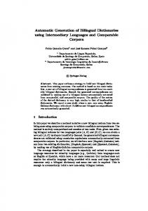
Fig. 1.
102
133
55
30
221
74
202
204 140
39
202
203 102
An example GE individuals’ genome represented as integers for ease of reading.
A number of variants of the PSA exist. The following paragraphs provide a description of the basic continuous version described by [2]. i. Initialize each particle in the population by randomly selecting values for its location and velocity vectors. ii. Calculate the fitness value of each particle. If the current fitness value for a particle is greater than the best fitness value found for the particle so far, then revise pbest. iii. Determine the location of the particle with the highest fitness and revise gbest if necessary. iv. For each particle, calculate its velocity according to equation 1. v. Update the location of each particle. vi. Repeat steps ii - v until stopping criteria are met. The update algorithm for the velocity, v, of each dimension, i, of a vector is: vi‘ = (w ∗ vi ) + (c1 ∗ R1 ∗ (pbest − pi )) + (c2 ∗ R2 ∗ (gbest − pi )) (1) where, w = wmax − ((wmax − wmin)/itermax) ∗ iter
(2)
c1 = 1.0 is the weight associated with the personal best dimension value, c2 = 1.0 the weight associated with the global best dimension value, R1 and R2 are random real numbers between 0 and 1, pbest is the vector’s best dimension value to date, pi is the vector’s current dimension value, gbest is the best dimension value globally, wmax = 0.9, wmin = 0.4, itermax is the total number of iterations in the simulation, iter is the current iteration value, and vmax places bounds on the magnitude of the updated velocity value. Once the velocity update for particle i is determined, its position is updated and pbest is updated if necessary. xi (t + 1) = xi (t) + vi (t + 1)
(3)
After all particles have been updated, a check is made to determine whether gbest needs to be updated.
genome representation is used. A genotype-phenotype mapping is employed such that each individual’s variable length binary string, contains in its codons (groups of 8 bits) the information to select production rules from a Backus Naur Form (BNF) grammar. The grammar allows the generation of programs in an arbitrary language that are guaranteed to be syntactically correct, and as such it is used as a generative grammar, as opposed to the classical use of grammars in compilers to check syntactic correctness of sentences. The user can tailor the grammar to produce solutions that are purely syntactically constrained, or they may incorporate domain knowledge by biasing the grammar to produce very specific forms of sentences. BNF is a notation that represents a language in the form of production rules. It is comprised of a set of non-terminals that can be mapped to elements of the set of terminals (the primitive symbols that can be used to construct the output program or sentence(s)), according to the production rules. A simple example BNF grammar is given below, where is the start symbol from which all programs are generated. These productions state that can be replaced with either one of or . An can become either +, -, or *, and a can become either x, or y. ::= | ::= | | ::= |
+ * x y
(0) (1) (0) (1) (2) (0) (1)
The grammar is used in a developmental process to construct a program by applying production rules, selected by the genome, beginning from the start symbol of the grammar. In order to select a production rule in GE, the next codon value on the genome is read, interpreted, and placed in the following formula: Rule = Codon V alue % N um. Rules
yˆ ∈ (y0 , y1 , ..., yn )|f (ˆ y ) = max (f (y0 ), f (y1 ), ..., f (yn )) (4) III. G RAMMATICAL E VOLUTION Grammatical Evolution (GE) is an evolutionary algorithm that can evolve computer programs in any language [4], [5], [6], [7], [8], and can be considered a form of grammar-based genetic programming. Rather than representing the programs as parse trees, as in GP [9], [10], [11], [12], [13], a linear
where % represents the modulus operator. Given the example individuals’ genome (where each 8-bit codon is represented as an integer for ease of reading) in Fig.1, the first codon integer value is 220, and given that we have 2 rules to select from for as in the above example, we get 220 % 2 = 0. will therefore be replaced with .
Biological System
Grammatical Evolution Binary String
DNA
TRANSCRIPTION Integer String
RNA
TRANSLATION Rules
Program / Function
Executed Program
Amino Acids
Protein
Phenotypic Effect
Fig. 2. A comparison between Grammatical Evolution and the molecular biological processes of transcription and translation. The binary string of GE is analogous to the double helix of DNA, each guiding the formation of the phenotype. In the case of GE, this occurs via the application of production rules to generate the terminals of the compilable program. In the biological case by directing the formation of the phenotypic protein by determining the order and type of protein subcomponents (amino acids) that are joined together.
Beginning from the the left hand side of the genome, codon integer values are generated and used to select appropriate rules for the left-most non-terminal in the developing program from the BNF grammar, until one of the following situations arise: (a) A complete program is generated. This occurs when all the non-terminals in the expression being mapped are transformed into elements from the terminal set of the BNF grammar. (b) The end of the genome is reached, in which case the wrapping operator is invoked. This results in the return of the genome reading frame to the left hand side of the genome once again. The reading of codons will then continue unless an upper threshold representing the maximum number of wrapping events has occurred during this individuals mapping process. (c) In the event that a threshold on the number of wrapping events has occurred and the individual is still incompletely mapped, the mapping process is halted, and the individual assigned the lowest possible fitness value. Returning to the example individual, the left-most in is mapped by reading the next codon integer value 240 and used in 240 % 2 = 0 to become another . The developing program now looks like . Continuing to read subsequent codons and always mapping the left-most non-terminal the individual finally generates the expression y*x-x-x+x, leaving a number of unused codons at the end of the individual, which are deemed to be introns and simply ignored. Fig.2 draws an analogy between GE’s mapping pro-
cess and the molecular biological processes of transcription and translation. A full description of GE can be found in [4]. IV. G RAMMATICAL S WARM Grammatical Swarm (GS) adopts a Particle Swarm learning algorithm coupled to a Grammatical Evolution (GE) genotypephenotype mapping to generate programs in an arbitrary language. The update equations for the swarm algorithm are as described earlier, with additional constraints placed on the velocity and dimension values, such that velocities are bound to ±VMAX=255, and each dimension is bound to the range 0 to 255. Note that this is a continuous swarm algorithm with real-valued particle vectors. The standard GE mapping function is adopted with the real-values in the particle vectors being rounded up or down to the nearest integer value, for the mapping process. In the current implementation of GS, fixed-length vectors are adopted, within which it is possible for a variable number of dimensions to be required during the program construction genotype-phenotype mapping process. A vector’s values may be used more than once if the wrapping operator is used, and in the opposite case it is possible that not all dimensions will be used during the mapping process if a complete program comprised only of terminal symbols is generated before reaching the end of the vector. In this latter case, the extra dimension values are simply ignored and considered introns that may be switched on in subsequent iterations.
V. E XPERIMENTS & R ESULTS Two classification problems from the literature are tackled using Grammatical Swarm to demonstrate proof of concept for the GS methodology. The first, Mushroom Classification, is a standard benchmark problem from the UCI Machine Learning Repository [14]. The second problem is from the domain of Bioinformatics, and involves the detection of promoter sequences in Eukaryotic DNA. The parameters adopted across the following experiments are c1 = 1.0, c2 = 1.0, wmax = 0.9, wmin = 0.4, CMIN = 0 (minimum value a coordinate may take), CMAX = 255 (maximum value a coordinate may take), and VMAX = CMAX (i.e., velocities are bound to the range +VMAX to VMAX). In addition, a swarm size of 30 running for 1000 iterations using 100 dimensions is used. The same problems are also tackled with Grammatical Evolution in order to get some indication of how well Grammatical Swarm is performing at program generation in relation to the more traditional variable-length Genetic Algorithm-driven search engine of standard GE. In an attempt to achieve a relatively fair comparison of results given the differences between the search engines of Grammatical Swarm and Grammatical Evolution, we have restricted each algorithm in the number of individuals they process, and using typical population sizes from the literature adopted for each method. Grammatical Swarm running for 1000 iterations with a swarm size of 30 processes 30,000 individuals, therefore, a standard population size of 500 running for 60 generations is adopted for Grammatical Evolution. The remaining parameters for Grammatical Evolution are roulette selection, steady state replacement, onepoint crossover with probability of 0.9, and a bit mutation with probability of 0.01. A. Mushroom Classification The data set for this problem is taken from [14], and contains samples of 23 species of gilled mushrooms from the Agaricus and Lepiota families. The aim is to generate a classifer to predict if a mushroom is poisonous or edible, with the data set containing 8124 mushroom instances. As such there are two classes, and 22 attributes associated with this problem. The dataset has been split into a training set of 6424 instances, and a test set of 1700 instances. The grammar adopted for this problem is given below, and results in the generation of a conditional statement, where the number of conditions is not specified a priori, and must be determined by the evolutionary automatic programming system. ::= if() guess=’poisonous’; else guess=’edible’; ::= () and () | () or () | ::= | | | | | | | |
| | | | | | | | | | | | | ::= var2==’b’ | var2==’c’ | var2==’x’ | var2==’f’ | var2==’k’ | var2==’s’ ::= var3==’f’ | var3==’g’ | var3==’y’ | var3==’s’ ::= var4==’n’ | var4==’b’ | var4==’c’ | var4==’g’ | var4==’r’ | var4==’p’ | var4==’u’ | var4==’e’ | var4==’w’ | var4==’y’ ::= var5==’t’ | var5==’f’ ::= var6==’a’ | var6==’l’ | var6==’c’ | var6==’y’ | var6==’f’ | var6==’m’ | var6==’n’ | var6==’p’ | var6==’s’ ::= var7==’a’ | var7==’d’ | var7==’f’ | var7==’n’ ::= var8==’c’ | var8==’w’ | var8==’d’ ::= var9==’b’ | var9 ==’n’ ::= var10==’k’ | var10==’n’ | var10==’b’ | var10==’h’ | var10==’g’ | var10==’r’ | var10==’o’ | var10==’p’ | var10==’u’ | var10==’e’ | var10==’w’ | var10==’y’ ::= var11==’e’ | var11==’t’ ::= var12==’b’ | var12==’c’ | var12==’u’ | var12==’e’ | var12==’z’ | var12==’r’ | var12==’?’ ::= var13==’f’ | var13==’y’ | var13==’k’ | var13==’s’ ::= var14==’f’ | var14==’y’ | var14==’k’ | var14==’s’ ::= var15==’n’ | var15==’b’ | var15==’c’ | var15==’g’ | var15==’o’ | var15==’p’ | var15==’e’ | var15==’w’ | var15==’y’ ::= var16==’n’ | var16==’b’ | var16==’c’ | var16==’g’ | var16==’o’ | var16==’p’ | var16==’e’ | var16==’w’ | var16==’y’ ::= var17==’p’ | var17==’u’ ::= var18==’n’ | var18==’o’ | var18==’w’ | var18==’y’ ::= var19==’n’ | var19==’o’ | var19==’t’ ::= var20==’c’ | var20==’e’ | var20==’f’ | var20==’l’ | var20==’n’ | var20==’p’
| var20==’s’ | var20==’z’ ::= var21==’k’ | var21==’n’ | var21==’b’ | var21==’h’ | var21==’r’ | var21==’o’ | var21==’u’ | var21==’w’ | var21==’y’ ::= var22==’a’ | var22==’c’ | var22==’n’ | var22==’s’ | var22==’v’ | var22==’y’ ::= var23==’g’ | var23==’l’ | var23==’m’ | var23==’p’ | var23==’u’ | var23==’w’ | var23==’d’
A plot of the mean best fitness for 30 runs can be seen in Fig.3, and the performance of the best evolved classifiers are presented in Table I. A true positive (TP) in this case is the correct classification of a mushroom as being poisonous, a true negative (TN) is correctly classifying a mushroom to be edible, a false positive (FP) is incorrectly classifiying a mushroom as poisonous, and a false negative (FN) is incorrectly predicting a mushroom to be edible. The best solution generated by Grammatical Swarm is given below, where a gill-size of ’n’ is broad, a spore-print-color of ’h’ is chocolate, and a gill-color of ’r’ is green. if( ( ( gill-size == ’n’ ) or ( spore-print-color == ’h’ ) ) or ( gill-color == ’r’ ) ) guess=’poisonous’; else guess=’edible’; TABLE I P ERFORMANCE OF THE
BEST RULES ON THEIR CORRESPONDING TRAIN
AND TEST SAMPLE DATA ON THE
Name GS - Train GE - Train GS - Test GE - Test
Fitness .96 .96 .95 .96
M USHROOM PROBLEM INSTANCE . TP 3013 3055 819 825
TN 3121 3121 799 799
FP 217 217 71 71
FN 73 31 11 5
B. Eukaryotic Promoter Sequence Detection Gene’s are the sequence of nucleic acid bases in the chromosome of animals, plants and microorganisms that are used to express a protein product. Gene expression or transcription is tightly regulated, ubiquitous in nature the RNA polymerase II (PolII) is the most common transcription initiator, and together with a set of accessory general transcription initiation factors (GTF’S) bind to core promoter DNA elements. The promoter element is a highly conserved sequence (e.g. the TATA box), which is common to both prokaryotic and eukaryotic systems and positions RNA PolII for transcription imitation. A single base change in this nucleotide sequence drastically decreases in vitro transcription of TATA containing promoters [15]. Approximately 70% of human promoters contain a TATA box located approximately 27bp upstream of a start site for transcription [16]. The problem is to automatically generate a
classifier to predict the presence or absence of a promoter in a given DNA sequence. The sequence of the promoter can be in two general positions regarding the position of the start of the gene. In one case the promoter is located near and often adjacent to the transcribed region of the gene and are known as proximal promoter sequences. Those that are located some distance from the transcription site of a gene are known as enhancer elements. Within the proximal promoter or transcription centres the architecture of the DNA is critical. As more sequence data is generated in the scientific field including the human genome published simultaneously in Nature and Science in 2001 [17], [18], and many other animal, plant, and bacterial genomes, the search for promoter sequences is ongoing through the analysis of DNA sequences deposited to gene banks such as the EMBL nucleotide sequence database [19]. A number of specialised databases also exist such as the Eukaryotic promoter database EPD [20] (available at http://www.epd.isb-sib.ch) that contains an annotated non redundant collection of eukaryotic PolII promoters, experimentally defined by a transcription start site. The data set adopted here was obtained from [21], where there are five recuts of the dataset each containing 178 examples of coding sequences, 113 examples of human promoter sequences, and 869 examples of intron sequences. The experiments are conducted using the promoter sequences and the coding region sequences as postive and negative examples of the promoter and non-promoter classes respectively. The first of the five recuts of the data is used as provided, where the first two thirds of each class were used for training and the final third in each case used for the out-sample dataset to test for generalisation. The grammar adopted for this problem is given below, and the meaning of each wildcard symbol is presented in Table II. As can be seen from the grammar, Grammatical Swarm in this case is generating regular expressions of variable length that are used to predict the presence or absence of a promoter. The DNA sequences of interest are passed to the generated regular expressions, with the result that DNA sub-sequences matching the regular expression are marked as promoter regions. No a priori knowledge regarding promoter sequence length or location is required to use this approach. ::= | | ::= * | W | R | S | Y | K | V | H | D | B ::= A | T | G | C
The single best evolved solution over the 30 runs is tested on the outsample dataset for overfitting, and the numbers of true positives (TP - correctly classified promoters), true negatives (TN - correctly classified non-promoters), false positives (FP incorrectly classified non-promoters), and false negatives (FN - incorrectly classified promoters) are calculated and used to generate sensitivity and specificity values according to the following equations.
Grammatical Swarm - Mushroom
Grammatical Swarm - Eukaryotic Promoters
1
0.8
0.75
0.9
0.7 0.8
0.6
0.5
Mean Fitness (30 Runs)
Mean Fitness (30 Runs)
0.65 GS - Best GS - Average GE - Best GE - Average
0.7
0.6
GS - Best GS - Average GE - Best GE - Average
0.55
0.5
0.4 0.45
0.3
0.4
0.2
0.35 0
Fig. 3.
100
200
300 400 500 600 700 Generation(GE) / Iteration(GS)
800
900 1000
0
100
200
300 400 500 600 700 Generation(GE) / Iteration(GS)
800
900 1000
Plot of mean fitness over 30 runs on the Mushroom problem instance (left), and the Eukaryotic Promoter problem instance (right).
TABLE II M EANING OF THE WILDCARD SYMBOLS USED IN
THE EXTENDED
GRAMMAR .
Wildcard W R S Y K V H D B *
Nucleotides A or T A or G C or G C or T G or T A or C or G A or C or T A or G or T C or G or T A or C or G or T
sensitivity =
TP TP + FN
specif icity =
TN TN + FP
A plot of the mean best fitness for GE and GS over 30 runs can be seen in Fig.3, and the performance of the best evolved classifiers in each case are presented in Table III alongside some well known promoter sequences from the literature [22], [23]. VI. D ISCUSSION Table IV provides a summary and comparison of the performance of Grammatical Swarm and Grammatical Evolution on each of the problem domains tackled. In both problems Grammatical Swarm’s performance is on a par with Grammatical
Evolution in terms of the quality of the classifiers generated. In terms of best fitness on the mushroom classification problem both algorithms’ performance is statistically equivalent according to a resampling t-test at the 5% level, although Grammatical Evolution has a better average fitness. On the promoter prediction problem Grammatical Evolution takes the edge on average producing better solutions than Grammatical Swarm. The key finding is that the results demonstrate proof of concept that Grammatical Swarm can successfully generate solutions to problems of interest. In this initial study, we have not attempted parameter optimization for either algorithm, but results and observations of the particle swarm engine suggests that swarm diversity is open to improvement. We note that a number of strategies have been suggested in the swarm literature to improve diversity [24], and we suspect that a significant improvement in Grammatical Swarms’ performance can be obtained with the adoption of these measures. Given the relative simplicity of the Swarm algorithm, the small population sizes involved, and the complete absence of a crossover operator synonymous with program evolution in GP, it is impressive that solutions to each of the benchmark problems have been obtained. When analyzing the results presented one has to consider the fact that the Grammatical Evolution representation is variable-length with individuals’ lengths restricted only by the machines physical storage limitations. In the current implementation of Grammatical Swarm fixed-length vectors are adopted in which a variable number of dimensions can be used, however, vectors have a hard length constraint of 100 dimensions. We intend to implement a variable-length version of Grammatical Swarm that will allow the number
TABLE III P ERFORMANCE OF
THE BEST EVOLVED REGULAR EXPRESSIONS ON THEIR CORRESPONDING TEST SAMPLE DATA COMPARED TO SOME WELL KNOWN
PROMOTER SEQUENCES FROM THE LITERATURE .
T HE SENSITIVITY ( SENS .) AND SPECIFICITY ( SPEC .) OF EACH EXPRESSION ARE
RegExp GE: WTAWADV GS: TAKADR TATA CAAT TAAC GGGCGG GGCGGG YYANWYY
Fitness .84 .77 .74 .54 .73 .65 .67 .61
TP 26 25 23 21 19 10 12 0
TABLE IV A
COMPARISON OF THE RESULTS OBTAINED FOR AND
G RAMMATICAL S WARM
G RAMMATICAL E VOLUTION AVERAGED OVER 30 CASE .
Mushroom GS GE Eukaryotic Promoters GS GE
RUNS IN EACH
Mean Best Fitness (Std.Dev.)
Mean Average Fitness (Std.Dev.)
0.93 (0.032) 0.94 (0.034)
0.83 (0.022) 0.92 (0.041)
0.74 (0.02) 0.76 (0.01)
0.68 (0.02) 0.74 (0.01)
of dimensions of a particle to increase and decrease over simulation time to overcome this current limitation. VII. C ONCLUSIONS & F UTURE W ORK This study demonstrates the feasibility of the generation of computer programs using Grammatical Swarm, and demonstrates its application to two classification problems. A performance comparison to Grammatical Evolution has shown that Grammatical Swarm is on a par with Grammatical Evolution, and is capable of generating solutions with much smaller populations, with a fixed-length vector representation, an absence of any crossover, no concept of selection or replacement, and without optimization of the algorithm’s parameters. This is very encouraging for future development of the much simpler Grammatical Swarm, and other potential Social or Swarm Programming variants. Future work will involve developing a variable-length Particle Swarm algorithm to remove Grammatical Swarms’ length constraint, conducting an investigation into swarm diversity, the impact of a continuous encoding over a discrete encoding variant such as presented in [25], and considering the implications of a social learning approach to the automatic generation of programs. R EFERENCES [1] Bonabeau, E., Dorigo, M. and Theraulaz, G. (1999). Swarm Intelligence: From natural to artificial systems, Oxford: Oxford University Press. [2] Kennedy, J., Eberhart, R. and Shi, Y. (2001). Swarm Intelligence, San Mateo, California: Morgan Kauffman. [3] Kennedy, J. and Eberhart, R. (1995). Particle swarm optimization, Proceedings of the IEEE International Conference on Neural Networks, December 1995, pp.1942-1948. [4] O’Neill, M., Ryan, C. (2003). Grammatical Evolution: Evolutionary Automatic Programming in an Arbitrary Language. Kluwer Academic Publishers.
TN 57 51 50 32 53 54 54 60
FP 3 9 10 28 7 6 6 0
FN 13 14 16 18 20 29 27 39
sens. .67 .64 .59 .54 .49 .26 .31 .0
ALSO INCLUDED .
spec. .95 .85 .83 .53 .88 .9 .9 1.0
[5] O’Neill, M. (2001). Automatic Programming in an Arbitrary Language: Evolving Programs in Grammatical Evolution. PhD thesis, University of Limerick, 2001. [6] O’Neill, M., Ryan, C. (2001). Grammatical Evolution, IEEE Trans. Evolutionary Computation. 2001. [7] O’Neill, M., Ryan, C., Keijzer M., Cattolico M. (2003). Crossover in Grammatical Evolution. Genetic Programming and Evolvable Machines, Vol. 4 No. 1. Kluwer Academic Publishers, 2003. [8] Ryan, C., Collins, J.J., O’Neill, M. (1998). Grammatical Evolution: Evolving Programs for an Arbitrary Language. Proc. of the First European Workshop on GP, 83-95, Springer-Verlag. [9] Koza, J.R. (1992). Genetic Programming. MIT Press. [10] Koza, J.R. (1994). Genetic Programming II: Automatic Discovery of Reusable Programs. MIT Press. [11] Banzhaf, W., Nordin, P., Keller, R.E., Francone, F.D. (1998). Genetic Programming – An Introduction; On the Automatic Evolution of Computer Programs and its Applications. Morgan Kaufmann. [12] Koza, J.R., Andre, D., Bennett III, F.H., Keane, M. (1999). Genetic Programming 3: Darwinian Invention and Problem Solving. Morgan Kaufmann. [13] Koza, J.R., Keane, M., Streeter, M.J., Mydlowec, W., Yu, J., Lanza, G. (2003). Genetic Programming IV: Routine Human-Competitive Machine Intelligence. Kluwer Academic Publishers. [14] Blake C.L., and Merz C.J. (1998). UCI Repository of machine learning databases. University of California, Irvine, Dept. of Information and Computer Sciences. http://www.ics.uci.edu/∼mlearn/MLRepository.html. [15] Wasylyk B and P. Chambon. (1981). A T to A base substitution and small deletions in the conalbumin TATA box drastically decrease specific in vitro transcription. Nucleic Acids Res. 9:1813-1824. [16] Bucher P. (1990). Weight matrix analysis description of four eukaryotic RNA Polymerase II promoter sequences. Nucleic Acids Res. 22:1000910026. [17] Venter J,C. et al. (2001) The sequence of the human genome. Science 291:1303-1351. [18] Lander E.S. et al. (2001). Initial sequencing and analysis of the human genome. Nature 409:860-921. [19] Baker W., van den Broek A., Camon E., Hingamp P., Sterk P., Stoesser G., and Tuli M.A. (2002). The EMBL nucleotide sequence database. Nucleic Acids Res. 28:19-23 [20] Schmid CD., Praz V., Delorenzi M., Prier R., and Bucher P. (2004). The eukaryotic promoter database EPD: the impact of in silico primer extension. Nucleic Acids Res. 2004 32: D82-D85. [21] http://www.fruitfly.org/seq tools/datasets/Human/promoter/. [22] Howard, D., Benson, K. (2003). Evolutionary Computation Method for Promoter Site Prediction in DNA. In LNCS 2724, Proceedings of GECCO 2003, pp. 1690-1701. Springer-Verlag. [23] Lewin, B. (1999). Genes VII. Oxford University Press. [24] Silva, A., Neves, A., Costa, E. (2002). An Empirical Comparison of Particle Swarm and Predator Prey Optimisation. In LNAI 2464, Artificial Intelligence and Cognitive Science, the 13th Irish Conference AICS 2002, pp. 103-110, Limerick, Ireland, Springer. [25] Kennedy, J., and Eberhart, R. (1997). A discrete binary version of the particle swarm algorithm. Proceedings of the 1997 Conference on Systems, Man, and Cybernetics, pp. 4104-4109. Piscataway, NJ: IEEE Service Center.