The automation of PDE-constrained optimisation and ... - Imperial Spiral

Imperial College London Department of Earth Science & Engineering

The automation of PDE-constrained optimisation and its applications Simon W. Funke October 2012

Supervised by: Dr. Matthew D. Piggott Dr. Patrick E. Farrell Dr. Peter A. Allison Dr. Gerard J. Gorman Submitted in part fulfilment of the requirements for the degree of Doctor of Philosophy in Computational Physics of Imperial College London and the Diploma of Imperial College London

Declaration

I herewith certify that all material in this dissertation which is not my own work has been properly acknowledged.

Simon W. Funke

i

Abstract

This thesis is concerned with the automation of solving optimisation problems constrained by partial differential equations (PDEs). Gradient-based optimisation algorithms are the key to solve optimisation problems of practical interest. The required derivatives can be efficiently computed with the adjoint approach. However, current methods for the development of adjoint models often require a significant amount of effort and expertise, in particular for non-linear time-dependent problems. This work presents a new high-level reinterpretation of algorithmic differentiation to develop adjoint models. This reinterpretation considers the discrete system as a sequence of equation solves. Applying this approach to a general finite-element framework results in an automatic and robust way of deriving and solving adjoint models. This drastically reduces the development effort compared to traditional methods. Based on this result, a new framework for rapidly defining and solving optimisation problems constrained by PDEs is developed. The user specifies the discrete optimisation problem in a compact high-level language that resembles the mathematical structure of the underlying system. All remaining steps, including parameter updates, PDE solves and derivative computations, are performed without user intervention. The framework can be applied to a wide range of governing PDEs, and interfaces to various gradient-free and gradient-based optimisation algorithms. The capabilities of this framework are demonstrated through the application to two PDE-constrained optimisation problems. The first is concerned with the optimal layout of turbines in tidal stream farms; this optimisation problem is one of the main challenges facing the marine renewable energy

iii

industry. The second application applies data assimilation to reconstruct the profile of tsunami waves based on inundation observations. This provides the first step towards the general reconstruction of tsunami signals from satellite information.

iv

Contents

Acknowledgements

xi

1. Introduction to PDE-constrained optimisation and the adjoint equations

1

1.1. Introduction . . . . . . . . . . . . . . . . . . . . . . . . . . . .

1

1.1.1. From simulation to optimisation . . . . . . . . . . . .

1

1.1.2. Computing derivatives of models . . . . . . . . . . . .

3

1.1.3. Contributions of this thesis . . . . . . . . . . . . . . .

4

1.1.4. Mathematical notation and assumptions . . . . . . . .

6

1.2. Techniques for computing derivatives . . . . . . . . . . . . . .

7

1.2.1. Tangent linear approach . . . . . . . . . . . . . . . . .

9

1.2.2. Adjoint approach . . . . . . . . . . . . . . . . . . . . . 10 1.2.3. Alternative approaches . . . . . . . . . . . . . . . . . . 10 1.2.4. Higher-order derivatives . . . . . . . . . . . . . . . . . 11 1.3. Developing adjoint models . . . . . . . . . . . . . . . . . . . . 12 1.3.1. Adjoint of the continuous equations . . . . . . . . . . 12 1.3.2. Computing derivatives with algorithmic differentation

16

1.3.3. Adjoint of the discretised equations . . . . . . . . . . . 20 1.4. Summary and overview . . . . . . . . . . . . . . . . . . . . . 22 2. A library for developing discrete adjoint models

25

2.1. Introduction . . . . . . . . . . . . . . . . . . . . . . . . . . . . 26 2.2. Motivation

. . . . . . . . . . . . . . . . . . . . . . . . . . . . 28

v

2.3. The fundamental abstraction . . . . . . . . . . . . . . . . . . 30 2.3.1. Examples . . . . . . . . . . . . . . . . . . . . . . . . . 31 2.3.1.1. Diffusion equation . . . . . . . . . . . . . . . 31 2.3.1.2. Burgers’ equation . . . . . . . . . . . . . . . 31 2.3.1.3. Time-dependent diffusion equation with exponential source term . . . . . . . . . . . . . 32 2.4. The discrete adjoint system . . . . . . . . . . . . . . . . . . . 33 2.4.1. Derivation . . . . . . . . . . . . . . . . . . . . . . . . . 33 2.4.2. Examples . . . . . . . . . . . . . . . . . . . . . . . . . 34 2.4.2.1. Adjoint of the diffusion equation . . . . . . . 34 2.4.2.2. Adjoint of the Burgers’ equation . . . . . . . 34 2.5. Using libadjoint . . . . . . . . . . . . . . . . . . . . . . . . . . 38 2.5.1. Annotation . . . . . . . . . . . . . . . . . . . . . . . . 38 2.5.2. Recording the forward solutions . . . . . . . . . . . . . 39 2.5.3. Function callbacks . . . . . . . . . . . . . . . . . . . . 40 2.5.3.1. Operator callbacks . . . . . . . . . . . . . . . 40 2.5.3.2. Callbacks for algebraic operations . . . . . . 44 2.5.4. Solving the adjoint system . . . . . . . . . . . . . . . . 44 2.5.5. Callback generation with algorithmic differentiation . 45 2.5.6. Verification and debugging . . . . . . . . . . . . . . . 46 2.5.7. Error handling . . . . . . . . . . . . . . . . . . . . . . 49 2.6. Description of the core algorithms . . . . . . . . . . . . . . . 50 2.6.1. Deriving the discrete adjoint equations . . . . . . . . . 50 2.6.2. Optimal checkpointing . . . . . . . . . . . . . . . . . . 51 2.6.2.1. Binomial checkpointing . . . . . . . . . . . . 54 2.6.2.2. Determination of required forward solutions in a checkpoint . . . . . . . . . . . . . . . . . 56 2.7. Examples . . . . . . . . . . . . . . . . . . . . . . . . . . . . . 58 2.7.1. Burgers’ model . . . . . . . . . . . . . . . . . . . . . . 58 2.7.2. Shallow water model . . . . . . . . . . . . . . . . . . . 62 2.7.2.1. Application to an idealised data assimilation problem . . . . . . . . . . . . . . . . . . . . . 64 2.8. Summary . . . . . . . . . . . . . . . . . . . . . . . . . . . . . 68 3. Automated generation of adjoint models in FEniCS

71

3.1. Introduction . . . . . . . . . . . . . . . . . . . . . . . . . . . . 72

vi

3.2. The FEniCS system . . . . . . . . . . . . . . . . . . . . . . . 74 3.3. Applying libadjoint to DOLFIN . . . . . . . . . . . . . . . . . 74 3.3.1. Annotation . . . . . . . . . . . . . . . . . . . . . . . . 75 3.3.2. Recording the forward solutions . . . . . . . . . . . . . 76 3.3.3. Callbacks . . . . . . . . . . . . . . . . . . . . . . . . . 77 3.3.4. User interface . . . . . . . . . . . . . . . . . . . . . . . 78 3.4. Implementation . . . . . . . . . . . . . . . . . . . . . . . . . . 79 3.4.1. Boundary conditions . . . . . . . . . . . . . . . . . . . 79 3.4.2. Parallelism . . . . . . . . . . . . . . . . . . . . . . . . 81 3.4.3. Limitations . . . . . . . . . . . . . . . . . . . . . . . . 81 3.5. Examples . . . . . . . . . . . . . . . . . . . . . . . . . . . . . 82 3.5.1. Burgers’ equation . . . . . . . . . . . . . . . . . . . . . 82 3.5.2. Navier-Stokes equations . . . . . . . . . . . . . . . . . 84 3.5.3. Gray-Scott equations . . . . . . . . . . . . . . . . . . . 86 3.6. Summary . . . . . . . . . . . . . . . . . . . . . . . . . . . . . 89 4. A framework for PDE-constrained optimisation

91

4.1. Introduction . . . . . . . . . . . . . . . . . . . . . . . . . . . . 92 4.2. The reduced optimisation problem . . . . . . . . . . . . . . . 93 4.3. Optimisation algorithms . . . . . . . . . . . . . . . . . . . . . 96 4.3.1. Broyden-Fletcher-Goldfarb-Shanno method . . . . . . 96 4.3.2. Sequential quadratic programming . . . . . . . . . . . 100 4.4. The optimisation framework . . . . . . . . . . . . . . . . . . . 101 4.4.1. User interface . . . . . . . . . . . . . . . . . . . . . . . 101 4.4.2. Implementation . . . . . . . . . . . . . . . . . . . . . . 103 4.5. Examples . . . . . . . . . . . . . . . . . . . . . . . . . . . . . 104 4.5.1. Distributed control of the heat equation . . . . . . . . 105 4.5.2. Distributed control of a non-linear, time-dependent PDE . . . . . . . . . . . . . . . . . . . . . . . . . . . . 108 4.6. Verification . . . . . . . . . . . . . . . . . . . . . . . . . . . . 110 4.6.1. Smooth control . . . . . . . . . . . . . . . . . . . . . . 112 4.6.2. Bang-bang control . . . . . . . . . . . . . . . . . . . . 113 4.7. Summary . . . . . . . . . . . . . . . . . . . . . . . . . . . . . 114 5. Layout optimisation of marine turbine arrays

117

5.1. Introduction . . . . . . . . . . . . . . . . . . . . . . . . . . . . 119

vii

5.2. Current methods in wind farm layout optimisation . . . . . . 121 5.3. Mathematical formulation as a PDE-constrained optimisation problem . . . . . . . . . . . . . . . . . . . . . . . . . . . 123 5.3.1. The governing PDE . . . . . . . . . . . . . . . . . . . 123 5.3.2. The turbine parameterisation . . . . . . . . . . . . . . 124 5.3.3. The functional of interest . . . . . . . . . . . . . . . . 125 5.3.4. Box and inequality constraints . . . . . . . . . . . . . 126 5.4. Numerical setup . . . . . . . . . . . . . . . . . . . . . . . . . 126 5.4.1. Optimisation algorithm . . . . . . . . . . . . . . . . . 126 5.4.2. Spatial discretisation . . . . . . . . . . . . . . . . . . . 127 5.4.3. Temporal discretisation . . . . . . . . . . . . . . . . . 128 5.4.4. Gradient computation . . . . . . . . . . . . . . . . . . 128 5.5. Verification . . . . . . . . . . . . . . . . . . . . . . . . . . . . 130 5.5.1. Verification of the forward model . . . . . . . . . . . . 130 5.5.2. Verification of the gradient computation . . . . . . . . 131 5.6. Examples . . . . . . . . . . . . . . . . . . . . . . . . . . . . . 132 5.6.1. A single turbine . . . . . . . . . . . . . . . . . . . . . 134 5.6.2. Scenario 1 . . . . . . . . . . . . . . . . . . . . . . . . . 135 5.6.3. Scenario 2 . . . . . . . . . . . . . . . . . . . . . . . . . 136 5.6.4. Scenario 3 . . . . . . . . . . . . . . . . . . . . . . . . . 140 5.7. Conclusions . . . . . . . . . . . . . . . . . . . . . . . . . . . . 140 6. Data assimilation for the shallow water equations with wetting and drying

143

6.1. Introduction . . . . . . . . . . . . . . . . . . . . . . . . . . . . 145 6.2. Shallow water model with wetting and drying . . . . . . . . . 146 6.2.1. Continuous formulation . . . . . . . . . . . . . . . . . 146 6.2.2. Spatial discretisation . . . . . . . . . . . . . . . . . . . 148 6.2.3. Temporal discretisation . . . . . . . . . . . . . . . . . 151 6.2.4. Verification . . . . . . . . . . . . . . . . . . . . . . . . 152 6.2.5. Volume conservation . . . . . . . . . . . . . . . . . . . 155 6.2.6. Validation . . . . . . . . . . . . . . . . . . . . . . . . . 156 6.3. The optimisation problem . . . . . . . . . . . . . . . . . . . . 156 6.3.1. Mathematical formulation as a PDE-constrained optimisation problem . . . . . . . . . . . . . . . . . . . . 156 6.3.2. Adjoint model implementation . . . . . . . . . . . . . 157

viii

6.4. Numerical examples . . . . . . . . . . . . . . . . . . . . . . . 158 6.4.1. Wave profile reconstruction on a sloping beach . . . . 159 6.4.1.1. Sinusoidal Dirichlet boundary . . . . . . . . 160 6.4.1.2. Composed sinusoidal Dirichlet boundary . . 162 6.4.2. Reconstruction of the Hokkaido-Nansei-Oki tsunami wave profile . . . . . . . . . . . . . . . . . . . . . . . . 165 6.5. Summary . . . . . . . . . . . . . . . . . . . . . . . . . . . . . 166 7. Summary and future work

169

7.1. Summary . . . . . . . . . . . . . . . . . . . . . . . . . . . . . 169 7.2. Future work . . . . . . . . . . . . . . . . . . . . . . . . . . . . 170 7.2.1. Application of libadjoint to other high-level frameworks170 7.2.2. Automated continuous adjoint approach in FEniCS

. 170

7.2.3. Using the automated adjoint derivation and the PDEconstrained optimisation framework . . . . . . . . . . 171 7.2.4. Support for multilevel methods for the PDE-constrained optimisation framework . . . . . . . . . . . . . . . . . 172 7.2.5. Support for solving optimisation problems in the unreduced form . . . . . . . . . . . . . . . . . . . . . . . . 172 7.2.6. Extensions of the optimal positioning of tidal turbines 172 7.2.7. Adjoint model of the Navier-Stokes equations with free-surface and wetting and drying

. . . . . . . . . . 173

A. Adjoint derivation of the continuous Burgers equation

175

B. Example usage of algorithmic differentiation

179

C. Adjoint derivation of the shallow water equations

183

References

187

ix

To my family

x

Acknowledgements

I thank my supervisors for the support during the development of this work. Dr Matthew Piggott was always very supportive and generous. I am grateful for his valuable advice and for giving me the opportunity to travel and participate in many conferences. Much of this research has been done in collaboration with Dr Patrick Farrell. He has not only been a great colleague and supervisor, but also became a good friend. His excellent ideas and invaluable contributions have greatly influenced the outcome of this thesis. I would like to thank Dr Peter Allison and Dr Gerard Gorman for their encouraging advice which they offered so readily. Furthermore, I would like to thank Dr David Ham who was always willing to discuss my research and give insightful advice. I thank Dr Marie Rognes for the invitation to the Simula Research Laboratory in Oslo. With Drs Farrell, Ham and Rognes emerged a fruitful collaboration which has formed the basis of this thesis. I would like to thank Prof. Christopher Pain for the support and help on the wetting and drying work. I also thank Prof. Zhu Jiang from the Institute of Atmospheric Physics, Beijing for his kind invitation to join the group research trip. Many thanks go to my colleagues of the Applied Modelling and Computation Group, who have been constantly supportive and I am very grateful for the good working environment they provided. I would like to thank Stephan Kramer for the valuable advice and Dr Jon Hill, Florian Rathgeber, Frank Milthaler, Sam Parkinson, Simon Leo Mouradian, Dave Robinson and Mark Goffin for proofreading parts of this thesis. Thanks also to Dr Tim Greaves and Surinder Singh Dio for making sure that the computer equipment was working.

xi

I gratefully acknowledge the support of the Grantham Institute for Climate Change and the Fujitsu CASE studentship, which funded me during the Ph.D. and provided complete freedom in my research. In addition, I acknowledge the Imperial College Trust for providing conference funding. I would have not been able to perform this work without the love and support of my family. The numerous visits and mails from my mother, father and my sisters, Leonie and Baucis, gave me the encouragement and support to finish this work. My father proofread this thesis with his enthusiasm, careful eye for detail and his mathematical mind. Finally, a very special thanks goes to my girlfriend, Kirsty. She always stood behind me, provided a stabilising force and helped me in difficult decisions. I cannot thank her enough for everything she has done and endured during these years.

xii

Chapter 1

Introduction to PDE-constrained optimisation and the adjoint equations Contents 1.1. Introduction

. . . . . . . . . . . . . . . . . . . . .

1

1.2. Techniques for computing derivatives . . . . . .

7

1.3. Developing adjoint models . . . . . . . . . . . . .

12

1.4. Summary and overview . . . . . . . . . . . . . . .

22

1.1. Introduction 1.1.1. From simulation to optimisation The use of computational models for simulating physical processes is a powerful complement to physical experiments. Firstly, they allow simulations that are impossible to perform in an experimental approach, such as climate physics or the dynamics of black holes and galaxies. Secondly, computational models can provide information that goes beyond what is observable by experiments, such as derivatives of the simulation result with respect to parameters. This thesis focuses on the computation of these derivatives

1

1. Introduction to PDE-constrained optimisation and the adjoint equations and their use in optimisation subject to computational models. The latter is motivated by the fact that many questions in science and engineering can be formulated as such optimisation problems. In engineering, the need for optimisation emerges regularly when seeking improved designs. A classical example is concerned with a key element in aeronautical engineering: What is the optimal shape of an aerofoil? In the pioneering work of Jameson (1988), this question is considered as an optimisation problem governed by the Euler equations for compressible flow. A similar design problem is investigated in chapter 5 of this thesis. It considers the situation where a large number of tidal turbines are to be deployed in a tidal stream. The investigated optimisation problem is: What are the optimal positions of the tidal turbines? A common task in geosciences is to determine unknown parameters such that the computer models best reproduces existing measurements (Ghil and Malanotte-Rizzoli, 1991). For example, satellite images provide detailed surface information about the ocean, but in general little is known about its interior (Stammer et al., 2000). The ECCO2 project aims to incorporate as much observations as possible to create an accurate description of the timeevolving state of the ocean (Menemenlis et al., 2008). Here, the problem formulation is: What is the state of the ocean at the beginning of the observation interval that minimises the difference between simulation and measurements? Chapter 6 of this thesis considers a related data assimilation problem where satellite observations of a tsunami inundation are available. The question here is: Is it possible to reconstruct the profile of the tsunami wave from the observed inundation pattern? Despite the variety of the considered tasks, they can all be formulated as optimisation problems constrained by partial differential equations (PDEs)

2

1.1. Introduction of the form: min J(u, m) u,m

(1.1)

subject to F (u, m) = 0, where m contains the optimisation parameters, J(u, m) ∈ R is the functional of interest that is to be minimised, and F (u, m) = 0 represents a PDE parameterised by m with solution u. As an example, reconsider the optimal design of the aerofoil. In this case, the parameter m contains the parameterised shape of the aerofoil, for example the coefficients of its Bézier curve. The physics are described by the Euler equations, which yield the pressure and velocity for a given aerofoil design. Finally, the functional of interest J computes the performance of the aerofoil, for example by evaluating the drag-lift ratio. The issue that the performance is to be maximised but formulation (1.1) describes a minimisation problem is resolved by minimising the negative of J. The presented examples have the common feature that the solution of the governing PDE is computationally demanding and that a large number of parameters need to be optimised. This makes solving these optimisation problems difficult and it became only recently tractable with the increase of computational power and the availability of efficient algorithms. In particular, a key role in this progress is the development of new gradient-based optimisation algorithms, such as Quasi-Newton methods (Nocedal and Wright, 1999, §6), and fast gradient computations with the adjoint approach (Errico, 1997).

1.1.2. Computing derivatives of models Gradient-based optimisation algorithms play a central role in solving PDEbased optimisation problems in practice. One difficulty in their application is that they require the derivative of the model output with respect to its input parameters. Table 1.1 lists some common techniques for computing this derivative information, together with an estimate of their computational expense. For the examples stated above and in many other applications, the number of input parameters is large, typically ranging from 102 (in the tidal turbine layout problem) up to 109 (in the ECCO2 example, where the parameter describes the initial state of the ocean (Stammer and Wunsch, 1999)) and more. At the same time, the number of output parameters can

3

1. Introduction to PDE-constrained optimisation and the adjoint equations Method Finite difference approximation Complex step approach Tangent linear approach Adjoint approach

Complexity (PDE solves) O(i) O(i) O(i) O(o)

Table 1.1.: Comparison of the required number of PDE solves for computing the derivative of a computer model with i input and o output parameters. The constant in front of the O operators is usually one. The PDE solves are typically the principle computational cost factor, and hence provide a good estimate for the total expense. In the given examples, i = 102 , . . . , 109 and o = 1 and hence the adjoint approach is by far the most efficient method. often be reduced to a single value of interest. For the examples above, these are the drag-lift ratio of the aerofoil, the norm of the difference between model and measurements and the power output of the tidal turbines. More generally, this is the case for any problem written in the form (1.1), since the functional of interest J yields a single value. Examining table 1.1 reveals that for such problems, the adjoint approach is the only practical option since the number of PDE solves is independent of the number of input parameters. Despite the advantages of the adjoint approach, its implementation is regarded as difficult and often combined with extensive development effort, even with the progress in algorithmic differentiation that aims to automate this process. In his recent book, Naumann (2012) states: [T]he automatic generation of optimal (in terms of robustness and efficiency) adjoint versions of large-scale simulation code is one of the great open challenges in the field of High-Performance Scientific Computing.

1.1.3. Contributions of this thesis The first chapters of this thesis present novel techniques for the automated derivation of adjoint models. By using a high-level reformulation of algorithmic differentiation, an automatic and robust way for deriving efficient adjoint models from models written in a high-level finite-element framework is obtained (chapters 2 and 3). Based on this, a framework for PDE-

4

1.1. Introduction constrained optimisation is developed, that is novel in terms of generality (both linear and non-linear, and both steady-state and time-dependent PDEs are supported) and its degree to which it is automated (chapter 4). This, together with a high-level language for the problem specification, drastically reduces the effort to solve PDE-constrained optimisation. The framework is applied to two applications for which adjoint-based optimisation has not been used before. Firstly, the optimal positioning of tidal turbines in a tidal stream (chapter 5), which results in new layout designs that have not yet been considered in the literature. Secondly, the application of data assimilation to wetting and drying processes in shallow water (chapter 6), which also has not been studied before. For this thesis, forward and adjoint models of the heat equation, the Burgers’ equation, the Navier-Stokes equations, the Gray-Scott equations and the shallow water equations with a wetting and drying extension have been developed, many of which have been used for PDE-constrained optimisation. The work in this thesis was partly undertaken with collaborators. The library libadjoint presented in chapter 2 was developed in joint work with P.E. Farrell and D.A. Ham. I was centrally involved in the whole design and development process and contributed large parts of the code, in particular to the core data structures and algorithms, the debugging tools. In addition, I was the sole developer of the checkpointing functionality for balancing the computation and storage cost. The integration of DOLFIN with libadjoint presented in chapter 3 is joint work with P.E. Farrell, D.A. Ham and M.E. Rognes. Again, I was centrally involved in the whole design and development process. Large parts of the code such as the Python interface to libadjoint, and the process of annotating and manipulating the equations solved, were performed in pair programming with P.E. Farrell. I was the sole author of major sections of dolfin-adjoint, including the checkpointing support and the optimisation framework presented in chapter 4. For all other work presented in this thesis, I am the sole contributor, in particular the turbine layout optimisation (chapter 5) and the application of data assimilation to wetting and drying processes (chapter 6). A publication based on the material in chapter 3, the integration of libadjoint in DOLFIN, has been accepted (Farrell et al., 2012). Furthermore, a wetting and drying scheme for the Navier-Stokes equations with free-surface has been developed and published as part of this Ph.D. (Funke

5

1. Introduction to PDE-constrained optimisation and the adjoint equations et al., 2011). This scheme will be briefly discussed in section 7.2.7. Publications based on the remaining chapters are in progress.

1.1.4. Mathematical notation and assumptions The adjoint approach is based on two components: the forward model and the functional of interest. In this thesis, the forward model is a (continuous or discretised) system of PDEs written in the abstract form: F (u, m) = 0 ∈ Z,

(1.2)

where F is the PDE operator that depends on the parameter m ∈ M and yields the solution u ∈ U in suitable Banach spaces M , U and Z. The parameter m might be a source term, initial or boundary conditions, the

geometry of the domain, or a coefficient that appears in the PDE. Although the adjoint system itself is independent on m, its introduction is useful for the following derivation and applications. In cases where the choice of the parameter m is irrelevant, it is sometimes neglected and the forward model is simply written as a function of u, i.e. F (u) = 0. The second ingredient is a scalar-valued functional of interest, which maps the PDE-solution and the parameter to a value of interest: J(u, m) ∈ R.

(1.3)

Similarly, the dependency on the parameter m is sometimes neglected and the functional of interest simply written as J(u). Throughout this thesis, it is assumed that the functional J and the PDEoperator F are continuously Fréchet differentiable. Fréchet differentiability is a generalisation of the differentiability from functions in Rn to Banach spaces: Definition 1. Let f : A ⊂ X → Y be an operator with Banach spaces X, Y

and A 6= ∅ open. f is called Fréchet differentiable if for all x ∈ A there exists a bounded linear operator Df (x) : X → Y such that: lim

khkX →0

6

kf (x + h) − f (x) − Df (x)hkY = 0. khkX

1.2. Techniques for computing derivatives f is continuously Fréchet differentiable if the function x → Df (x) is continuous.

In addition, it is assumed that the forward model (1.2) yields a unique solution u for any m ∈ M . This allows the definition of a solution operator

u(m), which maps the parameter m to the associated solution of the forward

model. Of course, for many PDEs the explicit form of u(m) is not known, and instead a program is used to compute an approximation. Substituting the solution operator u(m) into the functional of interest (1.3), yields the reduced functional : ˜ := J (u(m), m) . J(m)

(1.4)

An evaluation of the reduced functional of interest consists of first solving the forward model to obtain u and then evaluating J as in (1.3). It is also assumed that the linearised PDE operator ∂F (u(m), m)/∂u is invertible for any m ∈ M . The implicit function theorem shows that the

solution operator u(m) is then continuously Fréchet differentiable (Hinze et al., 2009, §1.4.2). A detailed discussion about the mathematical requirements for the adjoint approach can be found in (Hinze et al., 2009, §1.6). A final note on the notation of partial and total derivatives. If m consists of multiple entries arranged as a row vector m = (m1 , m2 , . . . ), then the total derivative is thought of as a row vector of the form: dJ = dm

dJ dJ , ,... dm1 dm2

.

.

Similarly, the partial derivative is in this case: ∂J = ∂m

∂J ∂J , ,... ∂m1 ∂m2

1.2. Techniques for computing derivatives This section derives the equations for computing the (total) derivative of the functional with respect to the parameters, i.e. dJ/dm. Taking the derivative of equation (1.4) and applying the chain rule on its right hand side yields:

dJ˜ dJ ∂J du ∂J = = + . dm dm ∂u dm ∂m

(1.5)

7

1. Introduction to PDE-constrained optimisation and the adjoint equations If equation (1.5) was used directly to compute the functional gradient, all three terms on the right hand side would be needed. For the terms involving J this is straightforward: the functional of interest is usually given as an explicit analytical formula from which the derivatives can be calculated. However, u(m) is only given implicitly through the solution operator and therefore du/dm is not directly accessible. One way to compute du/dm is obtained by taking the derivative of the forward model (1.2) with respect to m: ∂F du ∂F + = 0. ∂u dm ∂m

(1.6)

This equation contains the unknown du/dm and the derivatives of the forward model with respect to u and m. The PDE operator F is always available in explicit form from which the derivatives can be obtained. Since the linearised PDE operator ∂F /∂u is assumed to be invertible, the following equation for du/dm is obtained: du ∂F −1 ∂F =− . dm ∂u ∂m

(1.7)

Substituting equation (1.7) into (1.5) yields an equation for the functional gradient with terms that can all be derived explicitly: =λ∗

z }| { dJ ∂J ∂F −1 ∂F ∂J =− , + dm ∂u |∂u {z ∂m} ∂m

(1.8)

=−µ

where the asterisk denotes the Hermitian transpose. The order in which the first term on the right hand side is evaluated leads to two different approaches: one involves solving the tangent linear model for µ, and the other one solves the adjoint model for λ. To facilitate the comparison of these two approaches, a dimensional analysis is performed in the following sections. For that, let |m| and |u| denote

the (finite) dimensions of the parameter m and the forward model solution

u, respectively. Figure 1.1 visualises the dimensions of the linear operators in the right hand side of equation (1.8).

8

1.2. Techniques for computing derivatives

λ

}|

z |u|

×

{

−1

|u| × |u|

|

×

|u| × |m|

{z µ

+

|m|

}

Figure 1.1.: The dimensions of the linear operators in the right hand side of equation (1.8), visualised for a finite-dimensional example. The tangent linear solution µ is a matrix of dimension |u| × |m| and requires the solution of m linear systems. The adjoint solution λ is a vector of dimension |u| and is obtained with a single linear solve.

1.2.1. Tangent linear approach The tangent linear approach computes the functional derivative by first solving the tangent linear model for µ: ∂F ∂F µ=− , ∂u ∂m

(1.9)

and then using equation (1.8) to obtain the sought gradient: ∂J ∂J dJ = µ+ . dm ∂u ∂m Note that the linearised forward model (1.6) and the tangent linear model (1.9) are equivalent and hence µ = du/dm. The computational cost of this approach is dominated by the solution of the tangent linear system (1.9). The dimensional comparison in figure 1.1 reveals that the right hand side of this linear system is a matrix with |m|

columns, corresponding to the number of parameters. One option to solve this system is to invert the linearised PDE operator ∂F/∂u explicitly (for example with a LU decomposition) and to perform a matrix-matrix multiplication to compute µ. Alternatively, |m| iterative solves can be performed

9

1. Introduction to PDE-constrained optimisation and the adjoint equations for each column in the right hand side of the tangent linear system (1.9). However, in both cases, the computational cost scales linearly with |m|.

The next section shows that the adjoint approach leads to a linear system

whose dimension is independent of the parameter m.

1.2.2. Adjoint approach The adjoint approach first solves the adjoint equation: ∂F ∗ ∂J ∗ λ= . ∂u ∂u

(1.10)

The adjoint solution λ is then used to compute the functional gradient using equation (1.8): dJ ∂F ∂J = −λ∗ + . dm ∂m ∂m

(1.11)

The dimensional analysis in figure 1.1 shows that the right hand side of the adjoint equation (1.10) always consists of a single column vector, corresponding to the scalar-valued functional of interest J. Hence, the computation of the adjoint solution λ requires only one linear solve, independent of the dimension of m. In fact, the adjoint equation (1.10) does not depend on the choice of m at all. Furthermore, since the adjoint system is based on a linearisation of the forward model, its computational cost is expected to be equal or less than that of the forward model. However, in practice the efficient implementation of an adjoint model is often difficult, as will be discussed in the section 1.3.

1.2.3. Alternative approaches Apart from the tangent linear and adjoint approaches, there are alternative ways to obtain the functional gradient. Two common methods are the finitedifference and the complex-step approaches which will be briefly discussed in this section. The finite-difference approach approximates the functional gradient in the direction δm by computing the difference quotient. The central-difference formula for example yields: ˜ ˜ + hδm) − J(m ˜ − hδm) dJ(m) J(m δm = + O(|h|2 ) dm h

10

as h → 0.

1.2. Techniques for computing derivatives The main advantage of the finite-difference approach is its easy implementation: the model can be treated as a black box since only functional evaluations are required. However, the determination of a suitable step length h can be difficult: from a mathematical perspective, h should be chosen as small as possible to improve the approximation, but due to numerical cancellation the smallest suitable h value is bounded by round-off errors (Nocedal and Wright, 1999, pp. 166–169). The complex-step approach (Lyness and Moler, 1967) avoids this problematic by using complex calculus. It considers the reduced functional in the complex plane and uses the Cauchy-Riemann equations to derive following approximation of the directional derivative: ˜ + ihδm) Im J(m ˜ dJ(m) δm = + O(|h|2 ) dm h

as h → 0.

Since no difference operation is performed, this evaluation is not subject to subtractive cancellation errors. From an implementation perspective the complex-step approach is more intrusive, since the underlying code must be modified to support complex numbers. It has been recently shown that this method is tightly related to the forward mode of algorithmic differentiation described below (Martins et al., 2003). Both the finite-difference and the complex step approach only yield approximations of directional derivatives. To obtain the full functional gradient, the directional derivatives for all basis vectors in the parameter space must be computed separately. As a consequence the computational complexity increases linearly with the dimension of m. Nevertheless, the finitedifference method is popular due to its straightforward implementation and is a useful verification tool, see section 2.5.6.

1.2.4. Higher-order derivatives It is possible to compute higher-order derivatives by recursively applying the adjoint or tangent linear approach to itself. A detailed derivation of secondorder adjoints can be found in Griewank and Walther (2008, §13.4), Hinze et al. (2009, §1.6.5) and Thevenin and Janiga (2008, §4.6). One application of second-order information is in the context of optimisation with PDE constraints, for example for design optimisation (Guillaume

11

1. Introduction to PDE-constrained optimisation and the adjoint equations and Masmoudi, 1994) and optimal control (Hinze and Kunisch, 2001; Raffard and Tomlin, 2005).

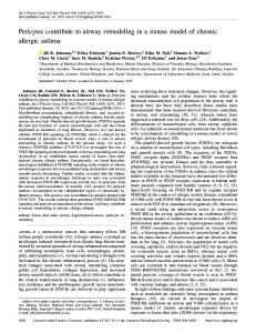
1.3. Developing adjoint models The implementation of an adjoint model is often complicated and can require years of development time for complex forward models. This section introduces different options for how the adjoint model can be derived and highlights their advantages and problems. The development of a PDE based forward model can be divided into three stages, as visualised in the top row of figure 1.2. First, it is decided which system of PDEs is to be solved. Then these equations are discretised in space and time. For that, a common choice is to first perform the spatial discretisation using the finite element method (Elman et al., 2005), and then apply a time stepping scheme such as Runge-Kutta methods (Ascher and Petzold, 1998). This separation of space and time discretisation is also known as the method of lines (Schiesser, 1991). The final step of the forward model development is the implementation of the discretised equations as source code. The adjoint model can be derived at any of these three stages, as shown in figure 1.2. The resulting adjoint system is at the same discretisation stage as the forward model from which it was derived. That is, the continuous adjoint is a continuous PDE, the discrete adjoint is a discretised PDE and the adjoint of the source code is an implementation of this discretised PDE. Interestingly, the diagram in figure 1.2 does not commute. As a result, the adjoint yields different solutions depending on how it was derived. The following sections discuss these options in more detail with a specific emphasis on how the derivation can be automated.

1.3.1. Adjoint of the continuous equations The continuous adjoint PDE is obtained by deriving the adjoint system of the continuous forward PDE prior to discretisation.

12

1.3. Developing adjoint models

continuous forward discrete forward −−−−→ −−−−→ forward code equations equations       libadjointy ADy y continuous adjoint equations   y discrete adjoint equations   y

discrete adjoint equations   y

adjoint code

adjoint code

adjoint code

Figure 1.2.: The adjoint system can be derived after any stage of the forward system development (top row). The derivation of the continuous adjoint is usually performed by hand. libadjoint is a library presented in chapter 2 that facilitates the development of the discrete adjoint. Algorithmic differentiation (AD) tools derive the adjoint model from the forward model source implementation. The resulting adjoint code and the adjoint solution depend in general on the stage at which the adjoint system was derived.

13

1. Introduction to PDE-constrained optimisation and the adjoint equations As an example, consider the time-dependent viscous Burgers’ equation with Dirichlet boundary conditions: ∂u + u · ∇u − ν∇2 u = 0 ∂t u=g u = u0

in Ω × (0, T ),

(1.12a)

on ∂Ω × (0, T ),

(1.12b)

for Ω × {0},

(1.12c)

where Ω ⊂ R defines the spatial and (0, T ) the temporal domain for the

solution u : Ω × (0, T ) → R, ν ∈ R is the viscosity parameter, g : ∂Ω × (0, T ) → R describes the Dirichlet boundary value and u0 : Ω → R the initial condition. The continuous adjoint of the Burgers’ equation with

respect to a functional of interest J(u, m) ∈ R reads as (see appendix A for a derivation): −

∂λ ∂J ∗ − (u · ∇)λ + (∇u)∗ λ − ν∇2 λ = in Ω × (0, T ), ∂t ∂u ∂J ∗ on ∂Ω × (0, T ), λ= ∂u ∗ ∂J λ= for Ω × {T }, ∂u

(1.13)

where ∇u denotes the Jacobian matrix of u and λ : Ω × (0, T ) → R is the adjoint solution. This adjoint PDE can be discretised and solved with similar techniques as the forward PDE. The continuous adjoint of the Burgers’ equation (1.13) reveals some general properties about the adjoint of a time-dependent problem: the resulting PDE is linear with initial conditions at the end of the time interval. Consequently it is solved backwards in time. Furthermore, the adjoint PDE depends on the forward solution u, and therefore the forward model must be solved beforehand. There are a few reasons why the derivation of the continuous level is preferable over its alternatives. Firstly, it allows the independent discretisation of forward and adjoint system. This flexibility can be important if the adjoint solution has different characteristics to the forward solution. Choosing different discretisation schemes and resolutions can increase the numerical accuracy for the same computational cost, see for example Pelletier et al. (2003); Fang et al. (2006).

14

1.3. Developing adjoint models The second advantage is that discontinuities introduced by numerical methods are unproblematic. A common example are upwind schemes to solve hyperbolic differential equations (Liu and Sandu, 2005), but also algorithms for space and time adaptivity are typically non-differentiable. Finally, the continuous adjoint plays an important role in shape optimisation as it avoids the issue of computing the derivative of the functional with respect to the mesh node positions (Anderson and Venkatakrishnan, 1999). However, this flexibility has the caveat that the functional gradient derived from the adjoint solution is generally not the functional gradient of the discrete forward model. An extreme case is presented in Gunzburger (2003, §4.1.2) where the functional gradient computed with the continuous adjoint

approach takes the opposite direction to the functional gradient of the discrete forward model. The reason for this inconsistency is that the forward and adjoint models are independently discretised. Hence, while forward and adjoint solutions converge to their continuous solutions, they can be arbitrarily unrelated if discretisation errors dominate. The consequences have been investigated by Griesse and Walther (2004) and Gunzburger (2003, §4.1.2) where the authors showed that this inconsistency can impact the

convergence of gradient-based optimisation algorithms. The manual derivation of the continuous adjoint system can be laborious for complex PDEs and the subsequent discretisation and implementation duplicates the development effort. This can become particularly problematic for models that are still in development: whenever the discrete forward system changes, the adjoint derivation has to be repeated and the adjoint model implementation updated. An automation of the continuous adjoint approach would need to be able to process the steps involved in the appropriate path in figure 1.2. The first step consists of the derivation of the continuous adjoint PDE from the forward PDE. This derivation can be automated, for example by using a symbolic algebra package such as SAGE (Stein et al., 2011). The second step, the discretisation of the resulting adjoint PDE, is more difficult to automate: the choice of a suitable discretisation scheme for a given PDE usually requires user expertise. Finally, the discretised equations must be passed to a code generation tool that automatically emits the adjoint model source code. While such tools are difficult to develop in general, there exists several

15

1. Introduction to PDE-constrained optimisation and the adjoint equations “problem solving environments” for the finite element method, for example FEniCS (Logg et al., 2011), Sundance (Long et al., 2012), GetDP (Dular et al., 1998), deal.II (Bangerth et al., 2007) and Analysa (Bagheri and Scott, 2004). Besides the potential of the continuous approach, the author is not aware of a software package that automates the required steps.

1.3.2. Computing derivatives with algorithmic differentation An alternative to the continuous adjoint approach is to postpone the derivation until the last stage of the forward model development, see figure 1.2. The resulting derivation operates at a much lower level: the source code. In this approach, the forward model is considered as a sequence of elementary instructions such as +, ·, sin or exp, for each of which the derivative

is known. That is, the reduced functional (1.4) can be written as a sequence of elementary instructions: ˜ J(m) = fp ◦ fp−1 ◦ fp−2 ◦ · · · ◦ f1 (m).

(1.14)

Differentiating equation (1.14) and applying the chain rule to its right hand side yields an equation for the functional gradient: ∂fp (mp−1 ) ∂fp−1 (mp−2 ) dJ˜ ∂f1 (m) = , ... dm ∂mp−1 ∂mp−2 ∂m

(1.15)

where mk is the k’th intermediate solution of equation (1.14), i.e. the result of the first k function compositions. There are two ways in which the right hand side of (1.15) is commonly evaluated. The first one, known as forward accumulation or forward mode, evaluates the terms from right to left. This evaluation involves only derivatives of elementary instructions for which the derivatives are known. The forward mode is tightly related to the tangent linear model (section 1.2.1): by observing that the reduced functional (1.4) can be written ˜ as J(m) = J(·, m) ◦ u(m), there exists a p0 such that u(m) = fp0 ◦ fp0 −1 ◦ · · · ◦ f1 (m), and hence dfp0 /dm = du/dm = µ appears as an intermediate

variable during the forward accumulation. The forward accumulation also adopts the dependency properties of the tangent linear model; in particular the calculation can be performed in line with the forward model without storing any additional intermediate variables.

16

1.3. Developing adjoint models The second way is to evaluate the right hand side of equation (1.15) from left to right, which is also known as reverse accumulation or reverse mode. This mode adopts the properties of the adjoint approach: in particular the gradient evaluation is performed backwards and all intermediate forward variables mi , i = 1, . . . , p must be stored. In contrast to the continuous adjoint approach, the gradient information obtained with this approach is consistent with the discrete forward model. That is, the computed gradient is the exact derivative of the forward model implementation. While this is generally desirable, in particular in the context of PDE based optimisation, there are cases where the consistent approach leads to an unsuitable discretisation of the continuous adjoint equation. Sirkes and Tziperman (1997) investigated this issue and present an example for which the adjoint solution contains numerical artifacts. The key advantage of this approach is that the derivation and evaluation of the adjoint model follow a completely prescriptive process, for which all required information is directly accessible from the source code. Consequently, the adjoint model can, in theory, be obtained fully automatically. This idea is implemented in automatic or algorithmic differentiation (AD) tools (Griewank and Walther, 2008), which commonly use one of the following techniques: Operator overloading. Uses the operator overloading feature of modern computer languages to build a tape of all executed functions and their arguments at runtime. This tape is then differentiated and evaluated to obtain the derivative information. This approach is relatively straightforward to implement but yields less efficient derivative code because no compiler optimisations can be performed on the differentiated code. Source to source compiler. A typical source-to-source AD tool takes the source code of the forward model as an argument and generates the source code for computing its derivative. Compared to operator overloading tools, source to source compilers tend to produce more efficient code but their implementation is more challenging. An example application of the source to source AD tool TAPENADE (Hascoët and Pascual, 2004) to a demonstration program can be found in appendix B.

17

1. Introduction to PDE-constrained optimisation and the adjoint equations An authoritative survey of the field can be found in Griewank and Walther (2008); Griewank (2003); Rall and Corliss (1996) and B¨ ucker et al. (2006). The main advantage of these low-level AD tools is that they can be applied directly to an existing forward model implementation. This is a major feature for complex models for which the manual derivation and implementation of the adjoint equations would be prohibitive. AD tools have been successfully applied to differentiate large models such as the MITgcm general circulation model (Heimbach et al., 2005), the FLUENT CFD code (Bischof et al., 2007), the CICE sea-ice model (Kim et al., 2006), and the WRF weather forecasting model (Xiao et al., 2008). However, their application have several limitations that need to be taken into consideration. Since these AD tools operate on the source code level they are typically designed for one specific programming language. In practice this raises two problems. Firstly, often only a subset of the programming language is supported, requiring the model developer to avoid advanced language features. For example, TAPENADE, a leading source to source AD tool for C and Fortran, prohibits the usage of dynamic memory allocations and pointer analysis in Fortran 95 in reverse mode (Hascoët and Pascual, 2004, §10.4). Secondly, it complicates the usage of multiple programming languages within the same model. A separate AD tool must be applied to the different parts of the code and manual intervention is needed to organise the differentiation between them. In particular, this can prohibit the use of external numerical libraries for which no differentiated version is available. The result of these restrictions can be seen in MITgcm, the flagship application for both the TAF (Giering and Kaminski, 2003) and OpenAD (Utke et al., 2008) source to source AD tools. Firstly, it is written in Fortran 77, which is fairly straightforward to parse. Secondly, the numerics are mostly explicit: the implicit step is self-adjoint (Heimbach et al., 2005), which means that no derivative code needs to be generated for the equation solve. Finally, the model has no hard dependencies on any external libraries, all of the core numerical calculations are performed within the model itself. Another issue for low-level AD tools is that they require significant expertise in both their usage and the forward model in order to derive efficient adjoint code. This is best explained by means of a simple example: consider a forward model that solves one non-linear system using the Newton method up to machine precision. Since the adjoint system is linear, an efficient ad-

18

1.3. Developing adjoint models joint implementation performs only one linear solve. Instead, without user intervention the AD tool differentiates every single Newton iteration. The result is that the adjoint model solves as many linear solves as there are Newton iterations in the forward model. This issue can be avoided by annotating the forward model with AD tool-specific directives to supply the necessary information. Heimbach et al. (2010) states that “work is thus required initially to make the model amenable to efficient adjoint code generation for a given AD tool. This part of the adjoint code generation is not automatic and can be substantial for legacy code, in particular if the code is badly modularized and contains many irreducible control flows”. The adjoint code produced by low-level AD tools is typically 3 to 30 times slower than the forward simulation (Naumann, 2012).

Finally, advanced features, such as the use of checkpoints to balance storage and computation costs that will be described in section 2.6.2, are often only implemented in mature AD packages and usually require further directives from the model developer (Kowarz and Walther, 2006; Hascoët and Araya-Polo, 2006). Also, support for parallel programs is still an active field of research (Hovland, 1997; Utke et al., 2009; Förster et al., 2011).

In summary, the adjoint derivation on the implementation level has the advantage that it can be automated if an AD tool is available. However, in practice multiple caveats appear and their application often requires extensive user intervention and expertise. Vidard et al. (2008) states his experiences of applying a low-level AD tool to the NEMO ocean model as: “Even for this simplified configuration, however, substantial human intervention and additional work was required to obtain a usable product from the raw [AD]-generated code . . . [The] memory management and CPU performance of the raw code were rather poor. . . . From that experience it has been decided to go toward the hand-coding approach”. These problems arise from the low abstraction on which the algorithmic differentiation is applied. By reasoning on the source code level, the differentiation tools have no high-level information about the forward model and hence have to handle low-level implementation details such as parallelism.

19

1. Introduction to PDE-constrained optimisation and the adjoint equations

1.3.3. Adjoint of the discretised equations

Motivated by the drawbacks of the previous two methodologies, this section and the following chapter attempt to circumvent their problems by choosing a different level of abstraction. On the one hand, it should be low enough such that the derivation of the adjoint system is a purely prescriptive process that can be automated. This is the case once the discretisation type has been chosen, along with the discrete function spaces for all variables. On the other hand, the abstraction should be as high as possible to avoid the implementation details of the forward model. From figure 1.2 it can be seen that deriving the adjoint from the discretised forward model matches these conditions. To illustrate the approach reconsider the time-dependent Burgers’ equation (1.12). Discretising with the finite element method in space and the forward Euler method in time, and linearising the non-linear advective term around the solution at the previous time level, yields the iteration: u0 = g, 1 1 M un+1 − M un + V (un )un + Dun = 0 ∆t ∆t

for n ∈ 0, . . . , N,

(1.16)

where the subscripts indicate the time levels, M is the mass matrix, −D is the discretised diffusion operator, V (un ) is the advection matrix assembled

at the velocity un , and N indicates the number of time step iterations. For brevity, define T (·) := −

1 M + V (·) + D. ∆t

(1.17)

The assignments (1.16) can be written as: 

I

 1 M T (u0 ) ∆t   T (u1 ) 

1 ∆t M

..

.

..

.

    u0 g      u1  0   =  .  u2  0     .. .. . .

(1.18)

The lower-triangular form of the matrix encodes the forward temporal flow of information in the equations: the solutions at later time levels depend on the solutions at earlier time levels, but not vice-versa.

20

1.3. Developing adjoint models Given a functional of interest J, the discrete adjoint equation of the forward model (1.18) is (the derivation is performed in section 2.4.2.2):        

I∗

T (u0 ) +

∂V (u0 ) ∂u0 u0

1 ∗ ∆t M

∗

T (u1 ) +

∂V (u1 ) ∂u1 u1

1 ∗ ∆t M

∗



λ0





∂J ∗ ∂u0



       ∂J ∗   λ1   ∂u    =  1 . ..    ∂J ∗  λ .  2   .   ∂u. 2  .. .. .. . (1.19)

This system recovers many of the properties of the continuous adjoint system (1.13). The adjoint operator is upper-triangular, hence the temporal flow of information in the adjoint system is reversed. Similarly to the continuous version, the discrete adjoint system depends on the forward solutions un . For this example, the discrete adjoint results in the same time discretisation scheme that was used for the forward model. To demonstrate this, the second equation in the adjoint system (1.19) is expanded: 1 1 M ∗ λ1 − M ∗ λ2 + V ∗ (λ2 ) + D∗ λ2 + ∆t ∆t

∂V (u1 ) u1 ∂u1

∗

λ2 =

∂J ∗ . ∂u1

It can be seen that the adjoint variable λ1 occurs only in the discretised time derivative term. Since the adjoint equations are solved backwards in time, this corresponds to a forward Euler method. In general, Sandu (2006) showed the discrete adjoint of explicit and implicit Runge-Kutta methods of any order p, result in a p-th order discretisation of the continuous adjoint. However, depending on the dynamics of the adjoint solution, this discretisation might be only appropriate for the forward model and result in numerical instabilities in the adjoint solution (Sirkes and Tziperman, 1997). The main advantage of deriving the adjoint from the discretised equations is that the process is completely prescriptive: once the forward model has been discretised, there is a defined procedure on how the associated adjoint model implementation is obtained. This property is the key for chapter 2, where a library is presented that automates this derivation. Another advantage is that, in contrast to deriving the adjoint from the source code, the derivation of discrete adjoint system is separated from its implementation. In particular, the operators in the adjoint equation (1.19) can be written in

21

1. Introduction to PDE-constrained optimisation and the adjoint equations multiple programming languages, rely on external libraries and be parallel aware. Finally, since the adjoint is derived on the discrete level, the resulting gradient information is consistent with the discrete forward model. Many optimisation algorithms such as SQP (section 4.3.2) and BFGS (section 4.3.1) rely on exact derivatives, and can fail to converge if only approximations are provided (Griesse and Walther, 2004); therefore, the consistency of the discrete adjoint approach is an important property for the remaining chapters of this thesis, where the gradients are used in the context of PDEconstrained optimisation.

1.4. Summary and overview The adjoint approach provides an efficient way to compute derivative information of PDE-based models in cases where the number of output values of interest is larger then the number of input parameters. Three approaches for developing the associated adjoint models have been introduced and their advantages and disadvantages discussed. The continuous approach provides most flexibility to the adjoint model developer, but requires usually a significant amount of development work. Alternatively, the adjoint model can be derived directly from the implementation of the forward model. Algorithmic differentiation tools aim to automate this process, however in practice their applicability can be limited and they often require user intervention. Finally, the discrete adjoint approach derives the adjoint model from the discretised forward equations. This approach has the advantage that the adjoint derivation is performed independently of implementation details. The remaining chapters are organised as follows. The next chapter introduces a software library that facilitates the development of adjoint models based on the discrete adjoint approach. Chapter 3 applies this library to a high-level finite-element framework, which results in an automatic, robust and efficient way of deriving and implementing adjoint models. This work is extended in chapter 4, in which a framework for rapidly setting up and solving PDE-constrained optimisation problems is developed. Chapter 5 applies this framework to the problem of finding the optimal positions of tidal turbines in a tidal stream. Another application is given in chapter 6, where a tsunami wave profile is reconstructed from observed inundation

22

1.4. Summary and overview pattern. Finally, chapter 7 makes some concluding remarks and presents future work.

23

Chapter 2

A library for developing discrete adjoint models Contents 2.1. Introduction

. . . . . . . . . . . . . . . . . . . . .

26

. . . . . . . . . . . . . . . . . . . . . .

28

2.3. The fundamental abstraction . . . . . . . . . . .

30

2.4. The discrete adjoint system . . . . . . . . . . . .

33

2.5. Using libadjoint . . . . . . . . . . . . . . . . . . .

38

2.6. Description of the core algorithms . . . . . . . .

50

2.7. Examples . . . . . . . . . . . . . . . . . . . . . . .

58

2.8. Summary . . . . . . . . . . . . . . . . . . . . . . .

68

2.2. Motivation

A publication based on this chapter is in preparation in collaboration with P.E. Farrell and D.A. Ham. The author was centrally involved in all aspects of the work.

25

2. A library for developing discrete adjoint models

Abstract This chapter presents a new software library that facilitates the development of adjoint models based on a high-level abstraction. Its fundamental concept is to consider the forward model as a sequence of equation solves. Based on this abstraction, the library builds a symbolic description of the forward model, from which it can automatically derive the symbolic representation of the associated adjoint model. The contained symbolic operators are then linked to implementations of these operators, with which the library can assemble and solve the adjoint equations. The chapter finishes with an application of this library to develop the adjoint of two example models, for which a direct low-level AD approach would be prohibitive.

2.1. Introduction The numerical core of a PDE based forward model typically consists of a sequence of equation assemblies and solves. However, the actual implementation of this functionality is often filled with machine-specific details, such as memory management, parallel communication and in-/output. As a consequence, the mathematical purpose of the model is interwoven with details on how it is to be implemented on a particular platform. A direct application of a low-level AD tool, which operates on the implementation level, needs to differentiate through all of these implementation details. This is the reason for many of the practical problems of applying such tools to complex models (see section 1.3.2), as the differentiation of the implementation details can be difficult. A typical example is the support of parallel communication which is a topic of active research in the AD community (Hovland, 1997; Utke et al., 2009; Förster et al., 2011). Section 1.3.3 described an alternative derivation of the adjoint model by considering the forward model as a sequence of equation solves. The main contribution of this chapter is the development of the library libadjoint, which uses this abstraction to facilitate and partly automate the development of adjoint models. The application of libadjoint to a forward model can roughly be divided into two steps. First, the forward model must be annotated, i.e. libadjoint functions are added to each equation solve in the forward model in order to pass some necessary information to libadjoint.

26

2.1. Introduction This information includes the structure of the equation, the variable it solves for and its linear and non-linear dependencies. As a result, libadjoint has a high-level representation of the forward model, also known as a tape. This tape is analogous to the concept of a tape in AD, except that instead of recording individual elementary operations, the units on the tape are whole equation solves. With the tape, libadjoint can derive the high-level representation of the associated adjoint equations; however, the operators in the derived adjoint equations are at that point just purely abstract handles. Therefore, the second development steps consist of providing implementations of all occurring operators. With these, libadjoint can then assemble and solve the adjoint equations. The advantage of this approach is that libadjoint’s representation of the forward equations is separate from implementation details. Consequently, the difficult derivation of the discrete adjoint system can be automated independently of details such as parallelism, external libraries, etc. The implementation of the required operators is usually relatively easy, and can be performed either manually or with the help of an additional AD tool. The library also manages the storage of forward and adjoint variables and supports the use of checkpointing algorithms to balance the storage and computation cost. Alternatively, libadjoint can be viewed as a high-level AD tool, where the elemental functions are arbitrarily complex and their derivatives and Hermitian transpose must be provided by the user. A related project is CasADi (Andersson et al., 2012), a symbolic framework for solving optimal control problems governed by ordinary differential equations with buildin algorithmic differentiation features. In this framework, the user builds a syntax tree by performing vector and matrix operations, which is then used to evaluate the function and its derivative. Another related project is YAO (Nardi et al., 2009). This project is motivated by finite difference schemes and regards the model as a repetitive execution of similar core functions, such as a computation on each grid point. By duplicating and connecting these modules, the forward and its associated adjoint model can be generated and executed. In contrast to these tools, libadjoint is specifically designed to be applied to existing forward models and focuses on computationally expensive models such as for solving PDEs.

27


2.2. Motivation To motivate the abstraction that libadjoint takes, the three options for developing an adjoint model introduced in section 1.3 are evaluated for two existing software packages: Fluidity, a computational fluid dynamics framework currently under active development (Piggott et al., 2008) and the FEniCS system, a collection of software components for automating the solution of PDEs by the finite element method (Logg et al., 2011; Logg, 2007). The application of the continuous adjoint approach (see section 1.3.1) to Fluidity is complicated by several factors. Fluidity is highly configurable about which and how equations are to be solved. In particular it supports the Navier-Stokes, the Stokes and the shallow water equations with various parametrisations and an arbitrary number of additional tracer equations. The application of the continuous adjoint approach would require the adjoint derivation for all these available options. Due to the low-level development approach, these adjoint equations would then have to be implemented manually. This difficulty is compound by the fact that the model is under active development. That is, the derivation and implementation of the adjoint model would have to be updated with every change in the forward model. Fluidity also allows the user to embed Python (van Rossum et al., 2008) code to specify runtime functionality of the forward model. For example, initial and boundary conditions, source terms, and diagnostic functions can be specified entirely in Python. Since the mathematical equations of this functionality are not known a priori, the continuous adjoint can not be derived for these features beforehand. The second alternative is to apply a low-level AD tool to Fluidity (see section 1.3.2). However, its source code has undergone years of development without consideration for the constraints that usually come with these AD tools. In particular the model is written in modern Fortran, and makes extensive use of advanced language features such as dynamic memory allocation, pointers, derived data types and function overloading. All of these are not supported by many AD tools. In addition linear equations are solved with the PETSc library (Balay et al., 1997, 2010), for which no differentiated version is available. For parallel execution, the model relies on MPI (Foster, 1995) whose differentiation is the topic of current research (B¨ ucker et al.,

28

2.2. Motivation 2004; Utke et al., 2009). All of these factors make applying currently available low-level AD tools to the whole model intractable. Finally, the approach of deriving and implementing the discrete adjoint equations as described in section 1.3.3 can be applied. By lifting up the abstraction from the source code level to equation solves, the implementation details can be avoided, while parts of the automatic derivation of the adjoint system can be preserved. Section 2.7 presents the successful application of this approach to the shallow water model of Fluidity. The second software package under consideration is FEniCS. In FEniCS, the user specifies the discrete problem in a high-level language, from which a dedicated finite element compiler generates efficient parallel code. The main problem of applying the continuous adjoint approach to FEniCS is that the equations to be solved are provided as user input and hence not known a priori. Therefore, an automation of this approach must derive the continuous adjoint system from the user input. However, the current implementation of the high-level language of FEniCS has no abstraction for time discretisation and hence the time loop is implemented manually. A general reconstruction of the continuous equation from this time loop is not straightforward. The application of a low-level AD tool is unfeasible for similar reasons to those for Fluidity: the control flow of a FEniCS model switches constantly between the driver program and the generated code. These difficulties are compound in the case of the Python interface of FEniCS where the code generation, compilation and execution happens dynamically at runtime. Furthermore, FEniCS is written in multiple different programming languages, exploits many modern programming language features and relies on external libraries, for example to solve the linear equations and to support parallelism, all of which make it difficult to apply a low-level differentiation tool. The alternative of deriving the adjoint model from the discretised equations avoids the advanced code generation pipeline in FEniCS. This option is particularly suited for this case, because the discrete adjoint approach and the high-level language of FEniCS operate on the same abstraction level. Chapter 3 presents the application of libadjoint to FEniCS in detail, which results in an automatic and robust way to derive the adjoint models.

29


2.3. The fundamental abstraction Motivated by the previous section and the advantages that the adjoint of the discretised equations offers (see section 1.3.3), the design of libadjoint is based on the fundamental abstraction that the forward model is a sequence of (linear or non-linear) equation solves. For that, it is assumed that the forward model (1.2) can be written as a sequence of possibly non-linear equations that are solved consecutively. The solution u is a block vector in which each block corresponds to the solution of one equation. The exact choice of the blocks and what is considered as one equation is left free to the developer. In a time-dependent forward model, each block could for example contain the solution of a specific time level. In the application of libadjoint to the FEniCS system, presented in the following chapter, each block corresponds to the solution of a user specified variational problem. While it would be possible to consider the forward model in the basic form (1.2), libadjoint expects the model cast in an extended, but equally expressive form: A(u)u = b(u),

(2.1)

where A is a block matrix, b is a block vector and u is the solution block vector. For example, the basic form (1.2) can be cast into this form by writing: Iu = Iu − F (u),

(2.2)

where I is the identity operator. The reason for using this extended form (2.1) is that it provides libadjoint explicit information about the linearity in equation (2.1). This can be an important optimisation as will be shown in section 2.5.3.1. The fact that the equations are solved consecutively, reveals more information about the structure of equation (2.1). An equation solve can only depend on previously computed solutions, and hence A is lower-blockdiagonal. For the same reason, the dependency arguments of a block row of A and b may only contain previously computed solutions and, for non-linear equations, the solution of the equation itself.

30

2.3. The fundamental abstraction

2.3.1. Examples The following three examples demonstrate how a discrete PDE model can be cast into form (2.1). 2.3.1.1. Diffusion equation The first example considers the steady diffusion equation given by: −∇2 u = f, subject to appropriate boundary conditions. Discretising with the finite element method results in the linear system: Du = M f,

(2.3)

where −D is the discretised diffusion operator, M is the mass matrix, and u and f are coefficient vectors for the solution and source term respectively.

Equation (2.3) can be trivially cast in the form of equation (2.1) by identifying A = D and b = M f . 2.3.1.2. Burgers’ equation In section 1.3.3 the Burgers’ equation discretised with a forward Euler time-discretisation was written in a form which directly conforms to equation (2.1). Now consider a backward Euler time-discretisation of the Burgers’ equation (1.12). One obtains following assignments (compare to (1.16)): u0 = g, 1 1 M un+1 − M un + V (un+1 )un+1 + Dun+1 = 0 ∆t ∆t

for n ∈ 0, . . . , N,

where the subscripts indicate the time levels, M is the mass matrix, −D

is the discretised diffusion operator, V (un+1 ) is the advection matrix assembled at the velocity un+1 , and N indicates the number of time steps. Each time step consists of the solution of a non-linear equation, that can be solved for example with the Newton method. There are two choices how this system can be cast into form (2.1). Either each Newton iteration is

31

2. A library for developing discrete adjoint models considered as one equation, which results in a set of linear equations (one equation per Newton iteration for each time step). Alternatively, the model can be directly considered as a sequence of non-linear equations. For that, define: R(·) :=

1 M + V (·) + D. ∆t

The assignments (1.16) can then be cast into form (2.1) as: 

I

 1 − ∆t M   

T (u1 ) 1 − ∆t M

T (u2 ) .. .. . .

    u0 g      u1  0   =  .  u2  0     .. .. . .

2.3.1.3. Time-dependent diffusion equation with exponential source term

Now suppose the forward model approximately solves the time-dependent diffusion equation with an exponential source term: ∂u − ∇2 u = eu , ∂t subject to the initial condition u(t = 0) = g and suitable boundary conditions. Discretising with the finite element method in space as above and the backward Euler method in time yields the iteration u0 = g, 1 1 M un+1 − M un + Dun+1 = E(un+1 ) ∆t ∆t

for n ∈ 0, . . . , N,

(2.4)

where subscripts denote time levels, ∆t is the time step, M is the mass matrix, −D is the discretised diffusion operator as before, E is the discretised exponential function, and N indicates the number of time steps.

The exponential operator can not be represented in the form A(u)u, and is therefore defined as part of the right hand side b(u). Writing the itera-

32

2.4. The discrete adjoint system tion (2.4) into form (2.1) yields: 

I

 1 − ∆t M   

1 ∆t M + D 1 − ∆t M



u0





g



     u1  E(u1 )      1  u2  = E(u2 ) . M + D ∆t     .. .. .. .. . . . .

(2.5)

Note that this representation is not unique: for example, the diffusion operator could be incorporated into the right hand side as part of b(u). However, it will later be seen that the formulation (2.5) minimises the number of required operator differentiations as it unveils that E is the only non-linear operator. In general, any discretised PDE may be cast in the form (2.1). For timedependent simulations, u is generally a block-structured vector containing the unknowns for all time levels, A is a matrix with a lower-triangular block structure containing the discrete operators, and b is a block-structured vector containing the right-hand side terms of the equations. However, this formulation does not imply that A and b are assembled and solved at once. For example, time-dependent forward models are typically solved from one time level to the next by iteratively assembling and solving one block-row of A and b. Similarly, libadjoint never demands to assemble the whole adjoint system. Instead, the adjoint equation is solved backwards from one time level to the next.

2.4. The discrete adjoint system 2.4.1. Derivation The discrete adjoint model is derived from the forward model cast in form (2.1). For that, let J(u) denote the real-valued functional of interest. Applying the definition of the adjoint equation (1.10) to the forward model (2.1) yields the general discrete adjoint system: (A + G − R)∗ λ =

∂J ∗ , ∂u

(2.6)

33

2. A library for developing discrete adjoint models where λ is the unknown adjoint solution, A is the left hand side of the forward model and G and R are defined as: ∂A ∂b G := . uj , R := ∂u ijk ∂u

(2.7)

For clarification the definition of G is given in tensor index notation. The equivalent block-wise definition is: Gik =

X ∂Aij j

∂uk

uj .

(2.8)

2.4.2. Examples The general discrete adjoint system (2.6) can be used to derive the adjoint equations for any forward system cast in form (2.1). This is now demonstrated on two examples from section 2.3.1.

2.4.2.1. Adjoint of the diffusion equation For the discretised diffusion equation (2.3), the operator A and the right hand side b do not depend on u, and hence G = R = 0. The resulting discrete adjoint system is therefore: D∗ λ =

∂J ∗ . ∂u

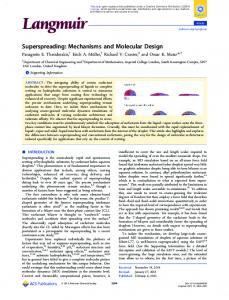
2.4.2.2. Adjoint of the Burgers’ equation Next, consider the discretised Burgers’ equation (1.18). For this example, the calculation of A∗ is trivial and R∗ = 0 as b does not depend on u. (∂J/∂u)∗ depends on the specific functional of interest. Therefore, attention is confined to the calculation of G. Once G is calculated, the calculation of G∗ is trivial. From the definition of G (2.7), the non-zero blocks of G are identified as: Gik 6= 0 ⇐⇒ block-row i of A depends on uk .

34

2.4. The discrete adjoint system Analysing the left hand side of the Burgers’ model (1.18) yields the blocksparsity pattern of the G matrix: 



0

 ∗ 0   ∗ 

0 .. .

..

.

  ,  

where ∗ denotes a non-zero block. To begin with, the top-left nonzero block,

G21 is calculated. G21 records the dependency of the second row of A on variable u1 , i.e. the dependency of the equation that solves for u1 on u0 . With the block-wise definition (2.8) the explicit form of G21 is obtained:

G21 =

=



u0



  u  0 ... ·   1 .. .

∂T (u0 ) ∂u0

∂T (u0 ) u0 . ∂u0

1 Both the mass operator M and diffusion operator D of T (·) = − ∆t M+

V (·) + D do not depend on u0 . Therefore, these terms vanish in the differentiation, and thus G21 simplifies to: G21 =

∂V (u0 ) u0 . ∂u0

(2.9)

By repeating this derivation for the remaining components of G, the full G matrix is obtained: 



0

 ∂V (u0 )  ∂u0 u0 G=  

0 ∂V (u1 ) ∂u1 u1

0 .. .

..

.

  .  

(2.10)

35

2. A library for developing discrete adjoint models Combining the contributions gives the full left hand side operator of the discrete adjoint system (2.6): 

   ∗ (A + G − R) =    

I∗

T (u0 ) +

∂V (u0 ) ∂u0 u0

1 ∗ ∆t M

∗

T (u1 ) +

∂V (u1 ) ∂u1 u1

1 ∗ ∆t M

∗



   . ..  .  .. . (2.11)

For these simple examples the derivation of the discrete adjoint model is not particular complicated. However, for a more complex forward model the manual derivation can become very extensive. In the case of the Burgers’ equation, one might want to use a high-order time discretisation, or couple it to another PDE. Both change the dependency structure and introduce additional block-rows in the recasted forward model, which complicates the derivation of the discrete adjoint. Furthermore, this derivation needs to be repeated every time the structure of the forward model changes, for example if the forward model is configurable at runtime. Despite its complication, the key property of this adjoint derivation is that it follows a completely prescriptive process: once the symbolic description of the discrete forward system in form (2.1) is available, the description of the associated adjoint system follows. Furthermore, if all block operators that occur in this symbolic description can be assembled, then each adjoint equation can be assembled and solved. In the Burgers’ example, the assembly of the adjoint operator (2.11) requires the block operators I ∗ , M ∗ , T ∗ (·) and ( ∂V∂·(·) ·)∗ and the adjoint right hand side requires the partial derivatives

of J.

The library libadjoint automates exactly that symbolic derivation and facilitates the assembly and the computation of the adjoint equations. The application of libadjoint to a forward model can be divided into three steps: Annotation The annotation builds an internal tape with high-level information about each equation solve that was performed during the forward model. Once the annotation is finished, libadjoint has a symbolic representation of the forward model in the form of (2.1). From this it can automatically derive a symbolic description of the associated adjoint system.

36

2.4. The discrete adjoint system Solve forward equation 1

Annotate equation 1

Record forward solution 1

libadjoint

Register callbacks

Solve forward equation 2 Figure 2.1.: A typical implementation of the three required steps for applying libadjoint to a forward model.

Recording the forward solutions The adjoint system depends in general on the forward solution. Consequently, libadjoint offers the functionality to record forward solutions that are required for assembling the adjoint operators.

Callback registration In order to solve the adjoint system, libadjoint must be able to assemble the block operators that occur in the symbolic representation. This is achieved by attaching function callbacks to the symbolic operators. The model developer must implement these operators according to libadjoint’s interface. Similarly, libadjoint uses function callbacks to perform algebra operations, such as vector addition or matrix multiplication.

Once the necessary information for these three steps has been provided, libadjoint can automatically derive, assemble and solve the adjoint system. The order in which the above steps are executed is free to the model developer. A common choice is to perform all three steps as the equation solve happens, see figure 2.1. These three steps will now be explained in further detail.

37


2.5. Using libadjoint This section discusses the necessary steps to apply libadjoint to a forward model. libadjoint is open-source and can be downloaded at https: //launchpad.net/libadjoint. The core of libadjoint is implemented in the C programming language for portability reasons, however additional interfaces to Fortran 90 and Python are available. The code examples in the following sections are presented in Python. Similar implementations in C and Fortran 90 can be found in the test directory of the libadjoint code base. A detailed description of all available libadjoint functions can be found in the manual (Farrell and Funke, 2011).

2.5.1. Annotation The purpose of the annotation is to build a tape with high-level information about each equation solved in the forward model. For that, libadjoint offers library functions that enable the model developer to express: the block structure of an equation; any non-linear dependencies of each block.

Each equation of the forward system is expressed using these functions and passed to libadjoint. The following code example shows an annotation of the first block equation of the discretised Burgers’ equation (1.18), with libadjoint specific functions marked red. 1

# Initialisation

2

adjointer = Adjointer()

3 4

# Create a symbolic representation of the identity operator

5

I = Block("IdentityOperator")

6

# Create a symbolic representation of the

7

# velocity vector at timestep 0

8

u = Variable('u', timestep = 0)

9

# Create a symbolic representation of the equation Iu = 0

10

e = Equation(u, [I], [u])

11

38

2.5. Using libadjoint 12

# Add the equation to the annotation

13

adjointer.register_equation(e) Note, that there is no need to annotate the right hand side of the Burgers’ forward model (1.18): it does not have any dependencies on u and is hence irrelevant for the adjoint system (however, it is required for the replay functionality that will be discussed in section 2.5.6). The annotation code for the remaining equations of the Burgers’ model (1.18) is similar and simply mimics the structure of the discrete system. In a practical implementation, the annotation calls are typically placed just before or after the associated equation is solved, see figure 2.1. The reason is that at this point usually all required dependency information is available. This also has the advantage that the annotation only happens if the associated equation is actually solved, which ensures that the annotation is always consistent with the forward model. This is particularly important for forward models that solve different equations depending on user configuration. Once the annotation has been executed, libadjoint has an internal symbolic representation of all forward equations and their dependencies in form (2.1).

2.5.2. Recording the forward solutions libadjoint needs to have access to the forward solutions in order to assemble and solve the adjoint equations. For that, the library offers functions to record the values of the forward variables. These function calls are naturally best placed directly after the equation solve in the forward model, see figure 2.1 Continuing the example code above, the following code shows how the initial velocity value in the Burgers’ example is recorded: 1

# Record the forward solution for the adjoint assembly

2

# Here "solution" contains the result of the associated

3

# forward equation

4

adjointer.record_variable(u, MemoryStorage(solution)) Storing the forward solutions for large models can require a significant amount of memory and so it is important to keep the memory footprint as low as possible. For that, libadjoint applies two strategies. Firstly,

39

2. A library for developing discrete adjoint models it only demands forward solutions on which the adjoint system depends and so only these need to be recorded. Secondly, the library automatically deletes forward solutions as soon as they are not required for any remaining calculations during the adjoint computation. In addition, libadjoint can use checkpoints that allow the recomputation of forward solutions instead of their storage. These checkpointing strategies will be discussed in section 2.6.2.

2.5.3. Function callbacks 2.5.3.1. Operator callbacks With the annotation, libadjoint can derive the structure of the adjoint system. It cannot, however, assemble and solve the adjoint equations. The operators mentioned in the annotation are at this point just abstract symbols to be manipulated. This problem is resolved by associating functions to each of the operators that perform the required tasks. The model developer must implement these functions with a defined interface, and attach them as callbacks to the symbolic operators. The specific required functionality that needs to be implemented depends on the linearity of the operator and where it occurs in the annotation. From the general discrete adjoint system (2.6) it can be seen that libadjoint needs callbacks to assemble each the terms A∗ , G∗ , R∗ and (∂J/∂u)∗ . Firstly, consider the term A∗ . Its assembly requires callbacks for each operator X that occurs in the annotation matrix A to: assemble the operator X ∗ or a matrix free representation thereof, if

the operator X occurs on the diagonal of A; compute its action on a given block vector v, i.e. X ∗ v, or a matrix

free representation thereof, otherwise. Usually, the implementation of these callbacks is straightforward, since the non-transposed operators are already available in the forward model. Their Hermitian transpose is either obtained manually or by using the built-in functionality of many linear algebra packages. Alternatively, the Hermitian transpose action callbacks can be derived by algorithmic differentiation as described in section 2.5.5. If the operators are symbolic objects, as is the

40

2.5. Using libadjoint case of the FEniCS framework presented in the next chapter, the required callback operations are obtained by simple symbolic manipulations. Next, consider the assembly of the G∗ contributions. For a non-linear operator X(v) that occurs as part of the annotation matrix A, callbacks are required to compute the Hermitian transpose of the Jacobian contracted with a

given block vector c, i.e. ((∂X/∂v) c)∗ , or a matrix free representation thereof, and compute its action on a given block vector w, i.e. ((∂X/∂v) c)∗ w, or

a matrix free representation thereof. The R∗ term assembly requires callbacks for any non-linear operator X(v) that is part of the right hand side b in the annotation system (2.1) to compute the Hermitian transpose of the Jacobian, (∂X(v)/∂v)∗ , or a

matrix free representation thereof. In practice, some of these derivatives are usually implemented in the forward model, for example if the Newton method is used to solve the non-linear equations. Otherwise, section 2.5.5 shows how the action callbacks can be obtained with automatic differentiation. If the operators are represented symbolically, as is the case in the following chapter, these callbacks are again obtained by simple symbolic manipulations. Finally, the right hand side of the adjoint system (2.6) requires a callback to compute the functional derivative (∂J/∂v)∗ for a given block vector

v, or a matrix free representation thereof. If this function is not available in the forward model, it can either be derived and implemented manually, or obtained with the help of automatic differentiation. The knowledge about linear and non-linear operators allows libadjoint to minimise the amount of code for which the derivative callbacks are required. For example, the highlighted operations in the following Burgers’ iteration from section 1.3.3 mark the code that needs differentiating if an AD tool is

41

2. A library for developing discrete adjoint models applied to the whole model:

1 M un+1 − ∆t

u0 = g,

1 M − V (un ) − D un = 0 ∆t

for n ∈ 0, . . . , N,

J(u1 , u2 , . . . ). With libadjoint’s annotation, the required derivatives reduce to only the non-linear operators, i.e.:

1 M un+1 − ∆t

u0 = g,

1 M − V (un ) − D un = 0 ∆t

for n ∈ 0, . . . , N,

J(u1 , u2 , . . . ) . The following code example implements and registers the identity callback for the Burgers’ equation (1.18). Since the identity operator appears on the diagonal, libadjoint requires a callback that assembles the corresponding block or a matrix free representation of it. An implementation that uses the numpy data structures (Oliphant, 2006) for vectors and matrices is:

42

2.5. Using libadjoint

1

# Define a callback following libadjoints specification

2

def identity(dependencies, values, hermitian,

3

coefficient, context):

4

# == "dependencies" and "values" ==

5

# Lists of forward solutions that are required for

6

# the assembly of nonlinear operators. In this case empty.

7

# == "hermitian" ==

8

# A boolean which indicates of the original or the

9

# tranpose operator is to be returned.

10

# == "coefficient" ==

11

# a scaling coefficient. libadjoint sometimes adds or

12

# subtracts operators in which case "coefficent" is != 1.

13

# == "context" ==

14

# User defined context information that can be passed

15

# to the callback

16 17

# Create the identity matrix with 100 entries

18

id_mat = Matrix(coefficient*numpy.eye(100))

19

# libadjoint also needs a vector to store the

20

# solution of the equation

21

id_vec = Vector(numpy.zeros(100))

22

return (id_mat, id_vec)

23 24

# Attach the callback to the identity block that was defined

25

# in the annotation code in section 2.5.1.

26

I.assemble = identity

Of course, in practice one would usually implement a matrix free representation of the identity operator instead. The callback function parameters contain all required information to perform the assembly. In particular, for non-linear operators, such as the advection operator V in the Burgers’ model (1.18), libadjoint passes the non-linear dependencies to the callback. In addition, the model developer can attach arbitrary data to the symbolic operators which is then passed to the associated callbacks via the context argument. In the example above, it might be useful to store the dimension

43

2. A library for developing discrete adjoint models of the matrix in the context. Other examples are the time step number, the current time, or accumulative statistics about the model. Further details about the callback interface can be found in the libadjoint manual (Farrell and Funke, 2011). 2.5.3.2. Callbacks for algebraic operations libadjoint needs to perform certain algebraic operations on vectors and matrices, such as addition, scaling and matrix-vector multiplication. For solving the equations, the library also needs to have access to appropriate solver routines. Similar to the operator callbacks from the previous section, libadjoint relies on user defined callback functions for these algebraic operations. The set of operations that the adjoint model developer must implement depends on the functionality used. The bare necessities include callbacks for matrixvector multiplication, and creating, deleting and adding vectors and matrices, as they are needed to assemble the adjoint equations. The automatic computation of the adjoint solution, presented in the next section, is based on a callback that implements an equation solver. For the checkpointing functionality discussed in section 2.5.6, libadjoint relies on additional callbacks for creating checkpoints and to read and write forward solutions from and to disk. Finally, the debugging tools discussed in section 2.5.6 require further callbacks such as the computation of the vector norm and to fill a vector with random values. While the implementation of these callbacks require a certain initial overhead of applying libadjoint to a new forward model, it allows libadjoint to remain lightweight and flexible towards any specific data structures. For data types for common libraries such as PETSc (Balay et al., 1997, 2010) and numpy (Oliphant, 2006), libadjoint comes with built-in implementations of these callbacks, which can be directly used by the adjoint model developer.

2.5.4. Solving the adjoint system After the steps described above, libadjoint has the necessary information about the forward model to derive, assemble and solve the associated adjoint system. The following code example demonstrates the user interface. The

44

2.5. Using libadjoint user first defines the functional of interest for which the adjoint system is to be derived. Then, the adjoint solutions can be computed by looping backwards over the equation indices, solving the associated adjoint equation and recording the result: 1

# Define a class that implements the functional of interest.

2

class MyFunctional(Functional):

3

def derivative(self, adjointer, variable, dependencies, values):

4 5

# This function must return the partial derivative of

6

# the functional with respect the forward variable

7

# "variable". It is used by libadjoint to add the

8

# adjoint source term to the right hand side of the

9

# adjoint equations.

10

...

11 12

J = MyFunctional()

13 14

# Loop backwards over all adjoint equations

15

for i in range(adjointer.equation_count)[::-1]:

16

# Derive, assemble and solve the i'th adjoint equation

17

(var, val) = adjointer.get_adjoint_solution(i, J)

18

# Record the adjoint solution

19

adjointer.record_variable(var, MemoryStorage(val)) The core function adj get adjoint solution performs four main steps. First, it derives the structure of the adjoint equation using the annotation. Second, if the equation contains any non-linear blocks it loads the required dependency values from the recorded forward solutions. It then calls the associated assembly and action callbacks to assemble the adjoint equation, and finally passes the result to the solver callback and returns the solution.

2.5.5. Callback generation with algorithmic differentiation This section demonstrates how the required action operator callbacks (section 2.5.3.1) can be automatically generated from C and Fortran code by applying a low-level AD tool to the associated assembly routines of the forward model. This is unnecessary in the case where the callbacks manage

45

2. A library for developing discrete adjoint models symbolic representations of the operators, such as in the FEniCS framework described in the next chapter. All of the action operator callbacks listed in section 2.5.3.1 can be generated using algorithmic differentiation. For example, assume the required callback is the Hermitian transpose action X ∗ v for a operator X that is part of the annotation matrix A, and a block vector v. For that, one implements a functional computing f (v, c) : = v ∗ (Xc) where c is a block vector. Applying an AD tool in reverse mode to compute the derivative of the functional f with respect to c yields the sought function df /dc = X ∗ v. A more complex computation arises for a non-linear operator X(v) that is part of the annotation matrix A. For this, an action callback is required that computes ((∂X/∂v)c)∗ w for block vectors v, w and c. This is achieved by first writing a functional f (v, w, c) := (X(v)c)∗ w. Applying and AD tool in reverse mode to compute its derivative with respect to v yields the required callback function. The remaining action callbacks for the contributions of R∗ and the right hand side (∂J/∂u)∗ are obtained in a similar way. While these assembly routines are typically amenable to AD tools, the restrictions of the low-level AD tool remains. In particular, the application of these tools becomes more complicated, if the assembly routines depend on external libraries such as MPI for parallelisation.

2.5.6. Verification and debugging Special attention has been drawn to provide verification and debugging tools for every stage of the adjoint model development with libadjoint. As a result, five features have been implemented that allow the quick identification and location of problems during the development and production stage of the adjoint model. Firstly, libadjoint offers to save detailed information about its current state to an HTML file, that can be viewed in any web browser. This file contains various information including a visualisation of the annotated forward and its derived adjoint model. An example HTML output produced from the Burgers’ annotation is shown in figure 2.2. In addition, the HTML output shows the registered callbacks and the forward and adjoint variables that are currently recorded. If a checkpointing scheme is used (see

46


(a) The forward matrix A (compare to equation (1.18)).

(b) The adjoint matrix (A + G − R)∗ (compare to equation (2.11)).

Figure 2.2.: The HTML output of libadjoint on the Burgers’ equation annotation. The green background denotes the diagonal blocks; and the grey background marks off-diagonal, nonzero blocks.

section (2.6.2)), further information about the checkpointed equations and their associated variables is included. This debugging tool is useful throughout the adjoint model development. In particular, it greatly facilitates the annotation process, since it allows a direct comparison of the annotation and the discrete forward model in form (2.1). Secondly, the library can verify the consistency of the annotation with the forward model. This test is based on the idea that libadjoint can use the annotation not only to derive and solve the adjoint system, but also to rerun the forward model. While doing so, it is asserted that the computed solutions are equivalent to the solutions that have been previously recorded from the forward model. For this feature to work libadjoint needs to have additional operator callbacks implemented that assemble the non-Hermitian transpose operators mentioned in the annotation and the right hand side of the forward equation (2.1). A successful execution of this test is a strong indicator that both the annotation and the implementation of the nonHermitian transpose operators are correct. The third debugging feature is used to verify the Hermitian transpose version of the callbacks. Given an operator X and its adjoint implementation X ∗ , libadjoint generates two random block vectors v, w with appropriate

47

2. A library for developing discrete adjoint models dimensions and checks whether following condition holds: hv, Xwi = hX ∗ v, wi .

(2.12)

An incorrect implementation of the Hermitian transpose is typically detected by repeating this test with a few different random vectors. Fourthly, libadjoint includes a test to check the implementation of callbacks that involve derivatives. The test applies a first-order Taylor expansion and asserts that the convergence order is as expected. The Taylor remainder convergence test is based on the observation that, given a nonlinear operator X(v), a dependency vector v and an arbitrary perturbation δv to the initial conditions p: kX(v + hδv) − X(v)k = O(|h|)

as h → 0,

X(v + hδv) − X(v) − h ∂X(v) δv = O(|h|2 )

∂v

as h → 0.

but that:

For a given vector v, libadjoint generates a pseudorandom perturbation vector δv with each component uniformly distributed and verifies the convergence orders for h → 0. This test is extremely sensitive to even slight errors in the implementation of the derivative callbacks. A typical case where this

test fails is if a non-linear derivative callback is generated with an AD tool, but has not been reapplied after changing the non-linear operator. Finally, the correctness of the adjoint solution can be verified by applying the Taylor remainder convergence test to the reduced functional of interest ˜ J(m) (definition (1.4)), i.e. the functional of interest considered as a pure ˜ function of a parameter m. After computing the functional gradient ∇J(m) from the adjoint solution with equation (1.11), the Taylor expansion states that:

but:

˜ ˜ J(m + hδm) − J(m) = O(|h|)

as h → 0,

˜ 2 ∗ ˜ ˜ J(m + hδm) − J(m) − hδm ∇ J(m) = O(|h| ) 48

as h → 0.

(2.13)

(2.14)


Traceback (most recent call last): [...] libadjoint.exceptions.LibadjointErrorNeedCallback: Could not find callback ADJ_BLOCK_ASSEMBLY_CB for operator M. (a) libadjoint throws this exception if a callback routine is missing (here the assembly callback for the mass matrix from the Burgers’ example) for one of the operators in the annotation.

Traceback (most recent call last): [...] libadjoint.exceptions.LibadjointErrorNeedValue: Need a value for u:1:0:Forward, but don't have one recorded. (b) This error occurs during the adjoint computation if an adjoint equation depends on a forward variable (here the forward solution of the second timestep and first non-linear iteration from the Burger’s example) which has not been recorded.

Comparing u:1:0:Forward against previously recorded value: norm of the difference is 1.648e+00 (> tolerance of 0.000e+00). (c) During libadjoint’s replay run, this error message indicates an inconsistency between original forward model and the annotated model.

Figure 2.3.: Python exceptions thrown by libadjoint for typical errors during the adjoint model development. The second-order convergence is very sensitive to implementation errors in the adjoint, and rigorously checks that the computed functional gradient is consistent with the discrete forward model. With the aid of these debugging and verification tools the development of the adjoint model becomes a step wise process after each of which its correctness can be verified.

2.5.7. Error handling One of the design concepts of libadjoint is to always check the prerequisites before performing a task. In case one of the requirements is not fulfilled, libadjoint stops its execution and informs the user. Some examples of errors that typically occur during the development phase are listed in figure 2.3. In particular, libadjoint returns an error if: a forward/adjoint solve contains an operator for which the required

callback is not registered; an adjoint solve depends on a forward variable which was not recorded;

49

2. A library for developing discrete adjoint models the replay test finds an inconsistency between the original forward

solution and the recomputation with libadjoint; one of the Taylor remainder convergence tests from the previous sec-

tion exceeds the defined tolerance. A detailed list of the errors and warnings can be found in the libadjoint manual (Farrell and Funke, 2011). In C and Fortran 90, the error handling is implemented by returning defined error codes; in Python, libadjoint throws an exception. This error handling further greatly simplifies the development process of the adjoint model: in many cases the developer can apply a “try and error” approach since the error messages given by libadjoint are often expressive enough to indicate what needs to be implemented next.

2.6. Description of the core algorithms This section discusses some details about the core algorithms used in libadjoint.

2.6.1. Deriving the discrete adjoint equations This section describes the core of libadjoint that derives and assembles the discrete adjoint system. The assembly of the adjoint system happens equation by equation with backward substitution, just as the forward system is solved equation by equation using forward substitution. That is, the k’th adjoint equation, the equation that solves for the adjoint solution λk , can be written as (compare to equation (2.6)): (A + G − R)∗kk λk =

∂J ∗ X − (A + G − R)∗kl λl . ∂uk

(2.15)

l,l>k

Algorithms 1 and 2 describe the procedures which libadjoint follows to assemble the left and right hand side of this equation, respectively. In order to avoid unnecessary assembly calls, these algorithms check in advance if an operator evaluates to zero, which occurs if the derivative of an operator is taken with respect to a variable on which it does not depend.

50

2.6. Description of the core algorithms ALGORITHM 1: Assembly of the left-hand side of the equation for λk Data: the index k of the adjoint equation to assemble Result: the left-hand side of the k’th adjoint system lhs G∗kk ← 0 ∗ Rkk ←0 if block row k of A has a dependency on uk then for all blocks Akj that depend on uk do G∗kk ← G∗kk +

∂Akj ∂uk uj

∗

end end if bk has a dependency on uk then ∗ ∂bk ∗ Rkk ← ∂uk

end ∗ lhs ← A∗kk + G∗kk − Rkk

2.6.2. Optimal checkpointing The adjoint operator in equation (2.6) consists of the term (A + G − R)∗ .

For a non-linear forward model, A will have dependencies on the forward solution and hence A∗ as well. Similarly, G∗ and R∗ may have complex dependencies on the forward solution. As a consequence, different parts of the forward solution must be available at different times when assembling the adjoint equations. While the straightforward approach of storing the whole forward solution is unproblematic for steady state problems, it can become prohibitively expensive for time-dependent simulations, since the storage requirement increases proportionally to the number of time steps. For example, storing a forward solution with 107 unknowns for 105 time steps on a standard computer requires over 7 TB. It is therefore apparent that the available storage would greatly constrain the number of time steps for which a real-world adjoint simulation could be run. One way to circumvent this problem is to use temporal interpolation.

Here, instead of storing all forward solutions, only solutions at selected time levels are kept. When the adjoint assembly requires an intermediate forward solution, a temporal interpolation scheme is used to approximate its value. Although the generality of this approach is questioned in Gunzburger (2003), it is sometimes used in hand-written adjoint codes. The adjoint of the NEMO ocean model is one such example (Vidard et al., 2008). Their experience shows that the necessary code manipulation “requires deep

51

2. A library for developing discrete adjoint models ALGORITHM 2: Assembly of the right-hand side of the linear system for λk Data: the index k of the adjoint equation to assemble Result: the right-hand side of the k’th adjoint system rhs ∂J ∗ rhs ← ∂u k for all blocks Alk 6= 0, l 6= k do rhs ← rhs −A∗lk λl end for all equations l that depend on uk , l 6= k do for all blocks Alj that depend on uk do rhs ← rhs −

∂Alj ∂uk uj

∗

λl

end for all l such that bl depends on uk , l 6= k do ∗ l rhs ← rhs + ∂b uk λl end end

knowledge of the original program and of the underlying equations . . . [and] introduces approximation errors into the computed derivatives, whose mathematical behavior is unclear” (Tber et al., 2007, §4.3). The problems associated with interpolation may be circumvented using checkpoints, from which the forward simulation can be restarted to recompute missing forward solutions. In the simplest checkpointing strategy, the complete time interval is split into a small number of equidistant subintervals and a checkpoint is stored at the beginning of each interval. When an intermediate forward solution is required for the adjoint assembly, the forward simulation is restarted from the closest preceding checkpoint and run until the required value is recomputed. An extension known as multi-level checkpointing applies this idea recursively: the time interval of the partial forward integration is again split into several subintervals on which checkpoints are stored, and so on. This multi-level checkpointing is successfully used in the MITgcm ocean model (Heimbach et al., 2005). Griewank (1992) proposed a strategy related to the multi-level approach in which the checkpoint distribution is based on a binomial interval splitting. By reusing the available checkpoint slots, a logarithmic growth of temporal and computational complexity is achieved, which is proven to be optimal (Grimm et al., 1996). Walther and Griewank (2004) showed that this approach is indeed advantageous over the multi-level checkpointing strategy

52

2.6. Description of the core algorithms and published a library named revolve that facilitates its implementation (Griewank and Walther, 2000). Both multi-level checkpointing and revolve allow the adjoint model user to balance the storage and computational complexity to their needs. However, this flexibility comes with additional development effort: the control flow constantly switches context between the forward and adjoint main loops, making the implementation of checkpointing more difficult than the temporal interpolation. While this can involve extensive development effort for a hand-written adjoint, the abstraction of AD is powerful enough to automatically generate the adjoint control flow according to the checkpointing strategy. Since the tape can be used to restart the simulation from a checkpoint, the checkpointing logic can be implemented within the AD tool. However, because the abstraction of low-level AD considers the model as a sequence of elementary instructions, it does not natively know about the concept of timestepping, which is required for efficient checkpointing. This information must therefore be provided by the model developer, often by explicitly adding AD-specific directives to the forward code. AD tools that offer checkpointing include TAF (Giering and Kaminski, 2002) and ADOL-C (Kowarz and Walther, 2006). As with low-level AD, libadjoint is sufficiently powerful to execute the required operations for checkpointing entirely within the library. In particular, the annotation and the supplied callbacks allow libadjoint to restart the simulation from a checkpoint. But in contrast to low-level AD tools, libadjoint’s annotation also provides the required time level information. This makes checkpointing with libadjoint available for almost no extra model development effort: the only requirement is to implement the callbacks for creating and deleting checkpoints. An implementation of this optimal checkpointing scheme within libadjoint faces several challenges. Firstly, it must be decided at which time levels the checkpoints should be placed. libadjoint uses the optimal checkpointing algorithm proposed by Griewank (1992) by interfacing to the revolve library (Griewank and Walther, 2000). The following section introduces this scheme. Secondly, it must be determined which forward solutions must be contained in a checkpoint. The checkpoints are used to restart the forward

53

2. A library for developing discrete adjoint models model, but they also need to store certain forward solutions for the adjoint computation. This problem will be discussed in detail in section 2.6.2.2. 2.6.2.1. Binomial checkpointing This section briefly describes the binomial checkpointing strategy implemented in revolve. It manages the control flow between forward and adjoint solves and finds the optimal checkpoint positions to minimise recomputation costs. The basic strategy, which assumes that the number of time levels is known a priori, is shown in algorithm 3. Clearly, the storage requirement of this algorithm is limited by the data required to store c checkpoints. The exact storage size depends on which forward solutions need to be included in the checkpoints. An execution of this algorithm for N = 10 and c = 3 is visualised in figure 2.4. The computational expense of algorithm 3 depends on the number of recalculations in the advance step. Therefore, the question arises where to optimally locate the checkpoints in order to minimise the number of recomputations. To answer this question, let t be the maximum number of how often any forward equation is solved in the advance steps. This number yields an upper bound for the computational cost. For example, if t = 2 the computational cost of the advance steps is less or equal than two full forward simulations. Now the question can be rephrased to: how large may the number of time levels N be for a fixed t? Griewank (1992) showed that

c+t N ≤ β(c, t) := . c

(2.16)

ALGORITHM 3: Binomial checkpointing Data: number of time levels N ; number of available checkpoints c Result: the adjoint solution Checkpoint equation 1 for k = N, 1, −1 do advance Run the forward model from the nearest checkpoint until equation k − 1. On the way, fill all free checkpoints using the binomial formula (2.16) as described below. reverse Solve the k’th forward and adjoint equation. If equation k − 1 is a checkpoint, free it. end

54

2.6. Description of the core algorithms 1

2

3

4

5

6

7

8

9

10

(*)

Figure 2.4.: Visualisation of binomial checkpointing strategy applied to N = 10 time levels and c = 3 checkpoints. The arrows show the temporal flow of the calculations: an arrow to the right (left) indicates the solution of one time step of the forward (adjoint) model. A (crossed) dot indicates the creation (deletion) of a checkpoint. This result is the key to find the optimal placement of checkpoints. Initially equation (2.16) is used to determine the smallest t that satisfies N ≤ β(c, t) for the given number of checkpoints c and time levels N . For the example

in figure 2.4, t = 2 satisfies this condition. To find the position for the second checkpoint (the first checkpoint is always for the first equation) in the example in figure 2.4, it is observed that the recomputations of the first checkpoint slot (marked with (∗) in figure 2.4) must be computable with at most t − 1 calculations per equation. The maximum number of time levels that can be computed with that restriction is β(c, t − 1) = β(3, 1) = 4,

and so the second checkpoint is placed at equation 5. The position of the third checkpoint is determined in the same way, but needs to take into account that one checkpoint less is available. Therefore, the third checkpoint

is placed β(c − 1, t − 1) = β(2, 1) = 3 time levels later. By recursively

applying this algorithm the full checkpoint positioning in figure 2.4 can be reconstructed.

This checkpointing distribution makes it possible to run large, timedependent adjoint models because β increases rapidly with larger c or t values in equation (2.16). For example, a simulation with 30, 000 time levels and 55 checkpoints results in a total cost of the advance steps that is at

55

2. A library for developing discrete adjoint models most three times the cost of one full forward run. With four times the cost of one forward model over 455, 000 time steps can be performed. Furthermore Griewank (1992) showed that under certain assumptions a trade-off between spatial and computational complexity can be obtained such that both the spatial and computational cost increase logarithmically with the number of time levels. The optimality of the method has been proven by Grimm et al. (1996). The revolve library implements two extensions of the basic binomial checkpointing strategy, both of which are supported by libadjoint. The first extensions allows the user to store some checkpoints in memory and some on disk. Saving checkpoints in memory has the benefit of a fast access time but its capacity is often limited. Disks are slower but usually have much larger storage capacity. The extension developed by Stumm and Walther (2009) manages the storage destination for the checkpoints. The second extension removes the assumption that the number of time levels is known a priori in algorithm 3. This is particularly important for forward models that apply time adaptive schemes where the number of time levels is only known after the first time integration. The checkpoint distribution for this case has been investigated by Stumm and Walther (2010).

2.6.2.2. Determination of required forward solutions in a checkpoint The checkpoints in algorithm 3 are created for two purposes, each of which can introduce dependencies on different forward solutions, that the checkpoint must contain. Firstly, they are used in the advance step to restart the forward model from their associated time level. Secondly, the reverse step uses them to access dependencies of the adjoint equation on forward variables that are not recomputed by the advance step. This makes it difficult to determine which forward variables need to be included in a checkpoint. However, libadjoint’s annotation is expressive enough to derived these dependencies automatically. Consequently, once the annotation of the forward model is complete, libadjoint handles the entire process of filling and freeing checkpoints internally, without user intervention.

56

2.6. Description of the core algorithms However, usually the annotation happens simultaneously with the forward solve (see figure 2.1). Therefore, during the annotation libadjoint can not determine which forward solutions to include in a checkpoint, since a future forward equation might depend on any previously computed solution. In that case, libadjoint requests the adjoint model developer to provide a list of forward solutions that need to be included in a checkpoint. The following checkpoint definition specifies which solutions libadjoint expects in this list. Definition 2. Let c be the index of a forward equation which is to be checkpointed. A checkpoint is a set of forward solutions ui with i < c, each of which is required for either: 1. solving a forward equation ≥ c or 2. evaluating an adjoint right hand side

∂J ∗ ∂uk

with k ≥ c.

Note that the first purpose of a checkpoint, being able to restart the forward model, is trivially fulfilled by the first condition in definition 2. However, the definition does not contain any explicit requirements to store dependencies of the corresponding adjoint equations, despite its right hand side. The following theorem shows that these dependencies are implicitly contained in the checkpoints. Theorem 1. A checkpoint for equation c contains all forward solutions ui , i < c that are required to assemble any adjoint equation ≥ c. Proof. Without loss of generality, the forward model is considered in the form:



F1



  F  F (u) =   2  (u) = 0, .. .

where each Fl corresponds to one equation in the forward model with solution ul . The forward propagation of information in the forward model ensures that any Fl only depends on forward solutions ui with i ≤ l.

Now, let k ≥ c. The k’th adjoint equation, the adjoint equation that

solves for λk , is (compare to equation (2.15)):

X ∂F ∗ ∂J ∗ . λl = ∂u kl ∂uk

(2.17)

l,l≥k

57

2. A library for developing discrete adjoint models The proof is complete if the checkpoint c contains all forward solution dependencies ui , i < c for this equations. The required dependencies to assemble the right hand sides are trivially contained in the checkpoint because of the second requirement in definition 2. Now consider the dependencies of the left hand side in equation (2.17). Assume that there is a (∂F/∂u)lk , l ≥ k that depends on ui with i < c. That is, the l’th forward equation Fl = 0, with l ≥ k ≥ c depends on

forward solution ui . The first requirement in definition 2 ensures that ui is contained in the checkpoint. This theorem greatly simplifies the task of providing the list of forward

solutions that must be included in a checkpoint since the adjoint operator dependencies can be ignored.

2.7. Examples The following examples demonstrate the application of libadjoint to two models that are included in Fluidity. Another application of libadjoint can be found in the following chapter, where the library is applied to the FEniCS system.

2.7.1. Burgers’ model As part of its developer training documentation, Fluidity includes a small example solver for the Burgers’ equation (1.12). The performed solutions steps are similar to the iteration (1.16), but uses two Picard iteration per time step to deal with the non-linear advective term: u0 = g, 1 1 0 M un+1 = M − V (un ) − D un for n ∈ 0, . . . , N, ∆t ∆t 1 1 0 M un+1 = M − V 0.5un + 0.5un+1 − D un for n ∈ 0, . . . , N. ∆t ∆t This model was adjoined as a proof-of-concept for libadjoint. The author is unaware of any current free low-level AD tool that is applicable to this model for the reasons explained in section 1.3.2. First, work was undertaken to

58

2.7. Examples implement the data callbacks, to allow libadjoint to manipulate Fluidity’s scalar, vector and tensor function objects (section 2.5.3.2). Since the required functions are common operations in the context of finite-element discretisations, these were already implemented in Fluidity. Consequently, the data callbacks are simply thin wrapper functions to the appropriate Fluidity routines. Next, a system was developed for model users to express their functional of interest. Fluidity embeds a Python interpreter (van Rossum et al., 2008) to provide dynamic programming facilities to model users. This was extended to provide a Python interface with which users could implement their own functionals of interest in a flexible and user-friendly manner. While this sacrifices some efficiency, these functionals are generally quite cheap to compute, and their cost is usually dominated by the cost of the forward and adjoint PDE solves. Then, the model was annotated using the techniques presented in section 2.5.1. The library calls for the annotation are distributed through the model, close to the code which they describe: the annotation of each nonlinear iteration happens within the non-linear iteration loop, the time step annotation happens within the time step loop, etc. At this point, the annotation was visualised in HTML (see figure 2.2) and inspected to ensure it matched the expectations of the model developer. Once the annotation was complete, the operator callbacks were implemented and registered as described in section 2.5.3.1. For the Burgers’ model the necessary operator callbacks are: an assembly and action callback for the identity operator I; an assembly callback for the term

1 ∆t M ;

an action callback for the timestepping operator T defined in (1.17); a callback providing the source terms for the replay test.

Matrices that do not change throughout the simulation, such as the mass and diffusion matrices, were cached. The advection matrix was reassembled at the arguments supplied. At this point, the annotation and callbacks were debugged by comparing the original model run against the forward replay mode of libadjoint (see section 2.5.6).

59

2. A library for developing discrete adjoint models Finally, the necessary derivative callbacks were supplied to libadjoint. Following callbacks were required: an action callback computing the derivative of the non-linear advection

operator V ; a callback for the derivative of the functional of interest.

The differentiation of the functional of interest was achieved with uncertainties, an object-overloading automatic differentiation tool for Python (Lebigot, 2011). Differentiating the non-linear advection term was more challenging, as the assembly function made extensive use of derived types which are poorly supported by free low-level AD tools. Instead, the advection assembly subroutine was rewritten in Fortran 77, and code for its derivative was generated with TAPENADE, a source-to-source AD tool (Hascoët and Pascual, 2004). Again, it is to be emphasised that no freely-available AD tool is capable of differentiating the entire model, and so the pure low-level AD approach is impractical. However, it was entirely practical to reimplement a Fortran 77 version of just the non-linear advection operator, as the amount of code to convert to an AD-differentiable form was very small. With the derivatives supplied, libadjoint successfully assembled each adjoint equation in turn, beginning at the end of simulation time and propagating backwards. The gradient of the functional with respect to various parameters (initial conditions, source terms) was computed with equation (1.11). For verification and benchmarking, the Burgers’ equation was solved in the domain interval Ω = [−10, 10] with initial condition u(x) = sin(xπ/5), viscosity coefficient ν = 1 and a time step size of ∆t = 1/32 for 0 ≤

t ≤ 1. The Burgers’ equation was discretised in space using the finite element method with piecewise linear basis functions on a uniform mesh

with 2 · 104 elements, and in time using the Crank-Nicolson scheme (Crank and Nicolson, 1947). The solutions of the forward model are shown in figure 2.5. Next, the functional of interest and control parameters were specified. The functional was defined to be: J(u, m) :=

Z

Ω

60

ku(t = 1)k2 dx,

(2.18)

2.7. Examples 1.0

-0.7 -0.5

0.5

0.0

0.0

-0.5 -0.5

-1.0 -10

-5.0

0.0

-0.7 -10 10

5.0

-5.0

0.0

5.0

10

(b) t = 1

(a) t = 0

Figure 2.5.: The forward solution of the Burgers’ example solved with Fluidity. 0.0010

0.0005

0.0

-0.0005

-0.0010 -10

-5.0

0.0

5.0

10

Figure 2.6.: The derivative of the functional of interest (2.18) with respect to the initial condition of the Burgers’ example. and the control parameter m was chosen to be the initial condition of u. The resulting functional gradient from the adjoint computation is shown in figure 2.6. The correctness of the adjoint solution and the functional gradient was verified with the Taylor remainder convergence test (2.14). The results, shown in table 2.1, show the expected second order rate of convergence and give confidence in the correctness of the adjoint implementation. Next, the efficiency of the implementation was benchmarked on one 2.13 GHz Intel Xeon CPU core with 12 GB memory. To obtain comparable timings for the forward and adjoint model without incorporating model specific overhead, the benchmark includes only the non-linear assembly, solver times and libadjoint related function calls. Specifically, the assembly of the linear operators is excluded, since they are assembled once in the initialisation step and then reused in both the forward and adjoint main loop. Moreover, the

61

2. A library for developing discrete adjoint models h

˜ 0 + hδu0 ) − J(u ˜ 0 )| |J(u

1 · 10−4 5 · 10−5 2.5 · 10−5 1.25 · 10−5

4.83 · 10−6 2.40 · 10−6 1.20 · 10−6 5.98 · 10−7

order

˜ 0 + hδu0 ) − J(u ˜ 0) |J(u ∗ ˜ 0 )| −hδu0 ∇J(u

5.38 · 10−8 1.35 · 10−8 3.63 · 10−9 8.40 · 10−10

1.01 1.00 1.00

order

2.00 2.00 2.00

Table 2.1.: The Taylor remainders for the reduced functional J˜ (i.e. the functional of interest (2.18) considered as a pure function of the initial condition u0 ) of the Burgers’ example. The perturbation direction δu0 is pseudorandomly generated. The expect order is one (two) for the remainder without (with) gradient information. Number of mesh elements Runtime of forward solve (s) Runtime of adjoint solve (s)

2 · 104 18 20

4 · 104 36 39

8 · 104 70 78

16 · 104 138 157

Table 2.2.: Runtime comparison of the forward and adjoint Burgers’ equation model with varying mesh resolution. The time step is fixed to ∆t = 1/32.

runtime of the embedded Python interpreter and I/O are excluded. The averaged results of four runs are given in table 2.2. They show that the adjoint model is only marginally slower than the original forward code, even though the G∗ contributions have to be assembled for the adjoint equations, which are not present in the forward run. For this example the adjoint implementation produced by libadjoint is therefore very efficient compared with the forward model.

2.7.2. Shallow water model Fluidity also includes a shallow water model which is significantly more complex than the Burgers’ equation solver presented in the previous section. The model solves the linear shallow water equations: ∂u + g∇η = 0, ∂t ∂η + H∇ · u = 0, ∂t

62

2.7. Examples where u and η are the unknown velocity and free-surface displacement and the parameters g and H are the gravity constant and the free-surface elevation at rest, respectively. The equations are discretised with the P1DG -P2 finite element pair, which is both LBB-stable and can represent geostrophic balance exactly. A full description of the model equations and their discretisation can be found in Cotter et al. (2009). Unlike the Burgers’ equation model, the shallow water model has more than one prognostic variable. The model is also made more complex by the fact that it solves on arbitrary oneor two-dimensional manifolds embedded in three-dimensional space, following the strategy of Bernard et al. (2009). As the shallow water model is also part of Fluidity, it was possible to use the data callbacks for Fluidity’s data types and the Python interface for implementing functionals from the previous work on the Burgers’ equation model. The forward model was annotated, and the callbacks implemented. For this work, the adjoint of the linear shallow water model is chosen, as the implementation of the non-linear term on arbitrary manifolds is still under development. Since almost all of the operators were cached by the forward model anyhow, the callbacks merely used these cached matrices. The only matrices not cached were the projection operators associated with the capacity to solve on arbitrary manifolds. The code for these projection operators was modularised to isolate the functionality in subroutines that the callbacks could use. The debugging features of section 2.5.6 were applied to detect potential implementation errors. The annotation of the forward model was verified by performing the forward replay test. Once this worked, the adjoint equations were assembled. An initial application of the Hermitian transpose consistency check (equation 2.12) indicated that the manifold projection operators were not self-adjoint. The required conjugate transposed projections were implemented by hand after which the Hermitian transpose consistency check passed. Finally, the correctness of the adjoint solution was verified using the Taylor remainder convergence test (2.14). Figure 2.3 shows the test results for the initial data assimilation configuration described in the next section. The Taylor remainder converged at second-order, giving confidence that the adjoint and gradient computations are correct.

63

2. A library for developing discrete adjoint models h

˜ est + hδη est ) − J(η ˜ est )| |J(η

1 · 10−4 5 · 10−5 2.5 · 10−5 1.25 · 10−5

1.87 · 10−5 9.33 · 10−6 4.67 · 10−6 2.33 · 10−6

order

1.00 1.00 1.00

˜ est + hδη est ) − J(η ˜ est ) |J(η est ∗ est ˜ −(hδη ) ∇J(η )|

5.47 · 10−10 1.37 · 10−10 3.42 · 10−11 8.55 · 10−12

2.00 2.00 2.00

Table 2.3.: The Taylor remainders for the reduced functional J˜ (i.e. the functional of interest (2.19) considered as a pure function of the initial condition of η) of the shallow water example. The perturbation direction δη est is pseudorandomly generated. The expect order is one (two) for the remainder without (with) gradient information.

2.7.2.1. Application to an idealised data assimilation problem

To demonstrate the functionality and efficiency of the shallow water adjoint model it was used to solve an idealised data assimilation problem. In data assimilation, some of the parameters specifying the problem are not exactly known. However, observations of the solution (possibly at different time levels if the problem is time-dependent) are available. The goal of data assimilation is to find a better estimate of the unknown input parameters for which the solution best “fits” the observations, usually in a least-squares sense. These kind of problems arise in many fields of geosciences, in particular in weather prediction (Park and Xu, 2009). This application is restricted to a simple shallow water setup in a twodimensional, doubly-periodic domain Ω = [0, 1]2 . In the considered problem, the initial value (at time t = 0) for the free-surface displacement η is unknown, while that of the velocity u is known. Given the observation of η at time t = 1/2 and t = 1 (an initial numerical experiment showed that the observation at t = 1/2 is essential for successfully solving the problem), the initial condition of η that recovers these observations is sought. Therefore, the functional of interest is defined as:

2

2

1

obs obs

J(η) := η t = − ηt= 1 + η(t = 1) − ηt=1

2 , 2 2 L (Ω) L2 (Ω) 64

order

(2.19)

2.7. Examples and the resulting optimisation problem is: min J(η est ) η est

subject to

(2.20a)

∂u + g∇η = 0, ∂t ∂η + H∇ · u = 0, ∂t u(t = 0) = u0 ,

(2.20b) (2.20c) (2.20d)

η(t = 0) = η est ,

(2.20e)

u(x = 0) = u(x = 1),

u(y = 0) = u(y = 1),

(2.20f)

η(x = 0) = η(x = 1),

η(y = 0) = η(y = 1).

(2.20g)

The minimum value of (2.20) is zero which is achieved if and only if the obs obs are exactly recovered. The constraints (2.20b) observations ηt=1/2 and ηt=1

and (2.20c) are the momentum and pressure equation of the linear shallow water equations. Equations (2.20d) and (2.20e) enforce the initial condition: u0 is the known velocity initial condition and η est is the estimate of the free-surface displacement initial condition. Finally, the equations (2.20f) and (2.20g) enforce periodic boundary conditions. This optimisation problem can be solved iteratively as follows. First, use the estimate η est to solve the shallow water model and its adjoint with respect to the misfit functional J. Then, equation (1.11) yields the derivative dJ/dη at the current point in parameter space. Finally, a gradient-based optimisation algorithm is applied to obtain a better estimate for η est , with which the procedure is restarted. For the following benchmarks, the LBFGS-B method (Byrd et al., 1995) of SciPy (Jones et al., 2001) was used as optimisation algorithm. No bounds or memory limit were specified, in which case the L-BFGS-B method is equivalent to BFGS. Starting with an initial estimate η est = 0, the optimisation loop was repeated until either the gradient norm of J was less than 10−12 or (J k − J k+1 )/ max(|J k |, |J k+1 |, 1) ≤ ,

where the superscript denotes the iteration of the optimisation loop and is a small multiple of the machine precision.

In order to verify the implementation of the solution procedure, its order of convergence was checked against theoretical results. For this, an analytical solution for problem (2.20) was constructed. By choosing g = H = 1, a

65


2.0

2.0

1.0

1.0

0.0

0.0

-1.0

-1.0

-2.0

-2.0

(a) Analytical initial layer thickness.

(b) Reconstructed initial layer thickness. 101 100 10-1

0.03

J

0.02 0.01

10-2 10-3 10-4

0.0

10-5 0

(c) Error in the reconstructed initial layer thickness.

5

10

15 20 Iteration

25

30

(d) Optimisation convergence plot.

Figure 2.7.: The results of the shallow water data assimilation problem with analytical solution. The optimisation starts with a zero initial guess for the initial layer thickness and successfully reconstructed the analytical function. The remaining errors are mainly caused by errors in the wave speed introduced by the time discretisation, and can be reduced by choosing smaller time steps.

periodic solution for equations (2.20b) and (2.20c) is given by: uexact =

! sin(2π(t + x)) sin(2π(t + y))

,

η exact = − sin(2π(t + y)) − sin(2π(t + x)). From this, the velocity initial condition and observations are derived: u0 = uexact (t = 0), obs ηt=1/2 = η exact (t = 1/2), obs ηt=1 = η exact (t = 1).

66

2.7. Examples Mesh element size L-BFGS-B iterations Rate of convergence for η est Rate of convergence for η(t = 1) Rate of convergence for u(t = 1)

0.3 24

0.3/2 27 2.0 1.6 2.3

0.3/4 29 2.3 2.2 2.2

0.3/8 31 + 9 2.1 2.2 2.3

Table 2.4.: Spatial order of convergence for the data assimilation problem. The time step size is 5 · 10−5 . The expected order is 2. The numerical results of the data assimilation problem with these analytical observations on a mesh with element size 0.3/4 and a time step of 1/32 are shown in figure 2.7. With a correct implementation, the solution of the optimisation problem is expected to converge to the analytical solution with the convergence rate given by the numerical analysis of the discretisation. The forward and adjoint shallow water problems were solved with the model described in section 2.7.2. The forward model uses Crank-Nicolson in time (Crank and Nicolson, 1947) and the P1DG -P2 finite element in space (Cotter et al., 2009). It has been shown that this discretisation choice yields a secondorder convergence in time and space (Cotter and Ham, 2011). However, any error in the implementation of the discretisation is likely to break either the spatial or temporal order of convergence. To derive the spatial order of convergence, the problem (2.20) was run with four different mesh resolutions and a small time step. The results are shown in table 2.4: as expected, second-order convergence is observed for both the control variable η est and the final state variables (to observe second-order convergence for η est with the highest resolution, it was necessary to perform 9 additional optimisation iterations after reaching the stopping criteria of the optimisation loop). The same technique was used to check the temporal order of convergence. The results in table 2.5 show again second order of convergence, giving high confidence in the correctness of the data assimilation implementation. To benchmark the efficiency of the implementation, the average time required to solve the forward and adjoint system was recorded. The problem was solved four times and the timing results averaged. Table 2.6 shows almost identical timings for both the forward and adjoint solves, which can be interpreted as follows: consider the shallow water model cast in the form given in equation (2.1). The linearity of the problem yields a forward opera-

67

2. A library for developing discrete adjoint models Time step (s) L-BFGS-B iterations Rate of convergence for η est Rate of convergence for η(t = 1) Rate of convergence for u(t = 1)

1/4 20

1/8 20 1.9 2.5 1.9

1/16 30 1.9 2.0 1.9

1/32 28 2.0 1.9 2.0

Table 2.5.: Temporal order of convergence for the data assimilation problem. The mesh element size is 0.3/16. The expected order is 2. Mesh element size Time step (s) Runtime of forward solve (s) Runtime of adjoint solve (s) libadjoint annotation time (s)

0.3/4 1/32 2.4 2.5 0.03

0.3/8 1/64 29 29 0.07

0.3/16 1/128 464 474 0.2

Table 2.6.: Averaged runtimes of the forward/adjoint solve and the total execution time of the libadjoint annotation in the data assimilation problem. tor A which is independent of the solution vector. The definition of adjoint G operators (2.7) yields that G = 0. Similarly, the right hand side b of equation (2.1) does not depend on the solution, yielding R = 0. Hence the adjoint operator is just the Hermitian transpose of the forward operator A, see equation (2.6). An efficient adjoint implementation is therefore expected to be approximately as fast as the forward equivalent. It is remarkable that even though the application of libadjoint has been performed without any optimisation, the benchmark timings suggest that the efficiency of the resulting adjoint model is very close to this best case assumption. Finally, the execution time of libadjoint to annotate the forward model was measured and was found to be less than 2% of the forward running time, see table 2.6.

2.8. Summary This chapter presented a library that facilitates and partly automates the development of adjoint models, based on the abstraction that the model is a sequence of equations solves. By annotating the forward model, libadjoint builds a symbolic description of the solved discrete system. With that, it can derive the symbolic description of the associated adjoint model. By

68

2.8. Summary providing implementations of the operators in this description, libadjoint can then assemble and solve the adjoint equations. The functionality was used to derive the adjoint of a Burgers’ and shallow water model for which low-level AD tools are not directly applicable. In these examples, libadjoint only partly automated the adjoint model development, as the annotation and the implementation of the operators had to be performed manually. The next section demonstrates how these steps can be entirely automated by applying libadjoint to a high-level finite-element framework.

69

Chapter 3

Automated generation of adjoint models in FEniCS Contents 3.1. Introduction

. . . . . . . . . . . . . . . . . . . . .

72

3.2. The FEniCS system . . . . . . . . . . . . . . . . .

74

3.3. Applying libadjoint to DOLFIN . . . . . . . . . .

74

3.4. Implementation

. . . . . . . . . . . . . . . . . . .

79

3.5. Examples . . . . . . . . . . . . . . . . . . . . . . .

82

3.6. Summary . . . . . . . . . . . . . . . . . . . . . . .

89

This chapter derives and expands upon P. E. Farrell, D. A. Ham, S. W. Funke, and M. E. Rognes. Automated derivation of the adjoint of high-level transient finite element programs. SIAM Journal on Scientific Computing, 2012. submitted The author was centrally involved in all aspects of the work.

71

3. Automated generation of adjoint models in FEniCS

Abstract This chapter presents the automatic derivation and implementation of adjoint models for finite element models written in the FEniCS system (Logg et al., 2011; Logg, 2007). In FEniCS, the discrete problem is represented as high-level data from which a dedicated finite element compiler generates optimised parallel code. The adjoint derivation is achieved by symbolic manipulation via libadjoint as described in the previous chapter. All required tasks for applying libadjoint are automated by inspecting the high-level problem specification of the forward model. The resulting adjoint model is represented in the same high-level formulation as the forward model and so the same finite element compiler can be applied. As a consequence, the adjoint model implementation is efficient and runs naturally in parallel. Multiple examples demonstrate the automation, robustness and efficiency of this approach.

3.1. Introduction The FEniCS system is a collection of software components for automating the solution of PDEs by the finite element method (Logg et al., 2011; Logg, 2007). The user specifies the variational form of the discrete equations in the domain specific language UFL (Alnæs, 2011), from which optimised finite element code is generated to compute their solutions. One of the key properties of this approach is that this high-level description can be algorithmically manipulated before the code generation is invoked. For example, the Newton solver in FEniCS makes use of this feature to form the Jacobian of the provided equations. The main contribution of this chapter is to exploit the high-level representation of the discrete forward system to automatically derive the associated adjoint model. This is achieved by integrating libadjoint (see chapter 2) into DOLFIN (Logg and Wells, 2010; Logg et al., 2011), the user front end of FEniCS. The software library presented here, dolfin-adjoint, inspects the high-level problem description provided by the user at runtime, and performs the required tasks for applying libadjoint automatically. The re-

72

3.1. Introduction FEniCS system

discrete forward equations −−−−−−−−−→ forward code   dolfin-adjointy

annotation, callbacks, recorded forward solutions   libadjointy

FEniCS system

discrete adjoint equations −−−−−−−−−→ adjoint code

Figure 3.1.: The automated generation of the adjoint model in FEniCS. The user specifies the discrete forward equations in a high-level language similar to mathematical notation (UFL (Alnæs, 2011)). During the forward simulation, dolfin-adjoint creates the required annotation and operator callbacks. From that, libadjoint derives the corresponding representation of the discrete adjoint equations in UFL. Both the forward and adjoint equations are then passed to the code generator of the FEniCS system to compute the forward and adjoint solutions.

sulting adjoint model is represented in the same high-level data format as the forward model. Therefore, the code generation techniques in FEniCS can be applied to the adjoint model as easily as to the forward model, see figure 3.1. Compared to applying libadjoint manually, this approach has the advantage that the derivation and solution of the adjoint model requires almost no user intervention. In addition, the adjoint derivation is generic: it applies to any PDE discretised with the finite element method, both to steady-state and time-dependent and both to linear and non-linear problems. Also, the adjoint model implementation is efficient and runs naturally in parallel, since it relies on the same code generation techniques as the forward model. Finally, the user has access to the checkpointing functionality and debugging tools implemented in libadjoint. The finite element environment Sundance (Long et al., 2012) is similar to FEniCS in that it also operates on variational forms. In particular, it can automatically differentiate and adjoin individual variational forms. However, this automation does not extend to cases where the model consists

73

3. Automated generation of adjoint models in FEniCS of a sequence of variational forms, as it is the typical case for time-dependent problems.

3.2. The FEniCS system This section gives a brief introduction to the FEniCS system with the relevant details for the remaining sections of this chapter. A thorough overview can be found in Logg et al. (2011). To solve a PDE with the FEniCS system, the user defines its discretised weak form in the domain specific language UFL (Alnæs, 2011), that mimics and encodes the mathematical formulation. This high-level formulation is then passed to a finite element form compiler such as FFC (Kirby and Logg, 2006), which generates optimised low-level code for the evaluation of the local element tensors. This generated code is used by DOLFIN to globally assemble and solve the problem. DOLFIN also provides the data structures for meshes, function spaces and functions. A list of commonly used DOLFIN functions is shown in table 3.1. For time-dependent PDEs, the temporal discretisation is usually performed with a non-finite element discretisation scheme. In this case, the user writes the time loop manually and solves the variational problem for each time level as described above. DOLFIN has interfaces for both C++ and Python. The Python interface uses just in time compilation, i.e. it invokes the code generation and compilation during runtime. In contrast, the code generation for the C++ interface happens as a preprocessing step before running the forward model. As a consequence, the high-level description of the forward problem is not directly available during runtime with the C++ interface. Because dolfin-adjoint relies on this data to perform runtime inspection and manipulation, the remaining sections discuss only the Python interface of DOLFIN.

3.3. Applying libadjoint to DOLFIN This section presents the software package dolfin-adjoint which integrates DOLFIN with libadjoint. In particular, dolfin-adjoint performs the annotation of the forward model, the recording of the forward solutions, and the

74

3.3. Applying libadjoint to DOLFIN DOLFIN function

Short description

solve(a == b, u, bcs) u.assign(v) assemble(a) bc.apply(A) solve(A, x, b) project(u, V)

Solve variational problem a(u, v) = b(u) ∀v Copy function v to u Assemble variational form Apply a boundary condition to a matrix Solve linear system Project u onto the function space V

Table 3.1.: Important DOLFIN statements relevant to dolfin-adjoint.

generation and registration of callback functions. All of these steps happen without any intervention by the model developer.

3.3.1. Annotation With the annotation, libadjoint collects the necessary information about the discrete forward system to symbolically derive the associated adjoint system (see section 2.5.1). More specifically, each equation solve in the forward model must be annotated, with information about which variable the equation solves for and its (possibly non-linear) dependencies on previously computed forward solutions. In dolfin-adjoint, the annotation happens automatically during the execution of the forward model. This is achieved by overloading all DOLFIN routines that modify the forward solution. These overloaded functions extract the required information from the UFL input and use the libadjoint interface to annotate the corresponding equation. It then calls the original DOLFIN routine and returns its result. All the DOLFIN routines listed in table 3.1 are overloaded by dolfin-adjoint. As an example, consider the solve routine that is used to solve linear and non-linear variational forms. A linear variational problem a(u, v) = b(v) ∀v may be solved by calling solve(a == b, u), where a is a bilinear

UFL form, b is a linear UFL form and u is the solution function. The overloaded solve routine annotates the corresponding linear equation as described in section 2.5.1. This annotation also contains information about the dependencies of operators in the equation on other forward variables, which dolfin-adjoint obtains by inspecting the associated UFL forms.

75

3. Automated generation of adjoint models in FEniCS The solve function can also be used to solve non-linear equations of the form F (u, v) = 0 ∀v, where F is a linear UFL form in v but non-linear in u. Calling solve(F == 0, u) automatically invokes the Newton method

to solve the non-linear system. Since libadjoint expects the annotation in the form of equation (2.1), dolfin-adjoint annotates the mathematically equivalent equation: Iu = Iu − F (u),

(3.1)

where I represents the identity operator. Alternatively, each iteration in the Newton solve could be annotated. However, this approach would be computationally less efficient as it yields an adjoint equation for each iteration in the Newton solve. In contrast, annotating equation (3.1) results in only one adjoint equation from its linearisation (Gilbert, 1992). Finally, the solve routine can be used to solve a linear system Ax = b where A is an assembled matrix and b an assembled vector. Such preassembly is commonly applied to avoid repeatedly assembling the same discrete operator if it occurs multiple times in the forward model. In this case, the overloaded solve function cannot examine the dependencies of the operators on other forward variables, since A and b are not UFL forms, but low-level matrix/vector objects without semantic information. This problem is resolved by also overloading the assemble routine in order to associate every assembled object with its UFL form. The overloaded solve routine then uses this association to find the corresponding UFL form of the assembled objects. That way, it can access all the required information and perform the annotation as in the cases above. DOLFIN provides alternative ways for solving variational forms by explicitly defining a solver object, such as NewtonSolver, KrylovSolver or LUSolver. dolfin-adjoint also overloads the solve routine of these classes and annotates the equations similar to the solve routine described above.

3.3.2. Recording the forward solutions As described in section 2.5.2, libadjoint requires the forward variables in order to assemble the adjoint system. By default, no checkpointing scheme is used and dolfin-adjoint records all forward variables. Similar to the annotation, this step is performed in the overloaded DOLFIN routines: after

76

3.3. Applying libadjoint to DOLFIN the original routine has been executed, the overloaded function records the solution as described in section 2.5.2 before returning the result. Alternatively, the user may use a checkpointing scheme to reduce the storage requirement by recomputing some of the forward variables. For that, libadjoint requests information about which forward variables to include in a checkpoint from the forward model. The exact requirements were specified in definition 2 of section 2.6.2.2. To be able to provide this information, dolfin-adjoint manages a list of forward variables that are currently in the program scope. When libadjoint requests the details about a checkpoint, dolfin-adjoint provides this list. It must be verified that this strategy fulfills the two requirements for a valid checkpoint given in definition 2. Firstly, the program scope obviously contains all forward variables that are required for future forward equations, and hence the first condition in definition 2 is satisfied. Secondly, the functionals of interest that are currently supported by dolfin-adjoint can all be P written in the abstract form J(u1 , u2 , ...) = k∈K j(uk ), where K denotes

all or a subset of the time levels and uk represents the forward variables of one time level. Therefore, the adjoint right hand side of the k’th adjoint equation (∂J/∂uk )∗ only depends on uk . Consequently, the second condition of definition 2 does not add further dependencies to the checkpoint.

3.3.3. Callbacks As discussed in section 2.5.3, libadjoint requires certain function callbacks for the operators that occur in the annotation of the forward system. In dolfin-adjoint, these callbacks are created simultaneously with the annotation of the forward model: when an overloaded DOLFIN function annotates an equation, it also generates all required callbacks for the operators that occur in this equation. The specific callbacks required depend on where the operator occurs in the annotation, see section 2.5.3. For example, if the operator is on the diagonal of the annotation, a callback for assembling its Hermitian transpose must be provided. Otherwise, a callback for computing the operator’s Hermitian transpose action to a given vector is required. For any operator that has dependencies on forward solutions, libadjoint requires callbacks for computing its derivatives. To support the replay functionality (section 2.5.6), libadjoint

77

3. Automated generation of adjoint models in FEniCS dolfin-adjoint statement

Short description

J = Functional(inner(u, v)*dx*dt) Functional(inner(u, v)*dx*dt[0:1]) Functional(inner(u, v)*dx*dt[1]) m = InitialConditionParameter(u) compute gradient(J, m) compute adjoint(J) compute tlm(m) adj checkpointing(...)

Functional hu, viΩ×(0,T ) Functional hu, viΩ×(0,1) Functional hu(t = 1), v(t = 1)iΩ Parameter for the initial velocity Computes the gradient dJ/dm Generator for the adjoint solutions Generator for the tangent linear solutions Configure checkpointing

Table 3.2.: Important dolfin-adjoint statements. The notation hu, viΩ := R u · v dx is used for the L2 inner product. Ω also requires callbacks for the non-Hermitian transpose operators and the right hand side of the forward model. In dolfin-adjoint, the operators are represented as UFL forms, which makes all these operations straightforward. For example, the adjoint variational form is obtained by swapping trial and test functions (Alnæs, 2011, §17.5.2). The generation of the derivatives employs the algorithmic differentiation capabilities of UFL (Alnæs, 2011, §17.7).

Besides these operator callbacks, libadjoint requires functions to perform algebraic operations such as addition, multiplication and solving variational problems. The implementation of these callbacks are thin wrappers around the corresponding DOLFIN functions and are independent of the specific forward model. In particular, the callback for solving equations consists of a thin wrapper around DOLFIN’s solve function that invokes the codegeneration for the assembly and solves the variational problem.

3.3.4. User interface After loading the dolfin-adjoint module and executing the forward model, the user has multiple options to compute and use the adjoint solution. A list of important dolfin-adjoint statements is given in table 3.2. A highlevel interface to dolfin-adjoint is compute gradient: given a Functional J and a Parameter m, it computes the gradient dJ/dm with the adjoint approach. Alternatively, the adjoint solution can be accessed directly by using the compute adjoint function. In addition, dolfin-adjoint supports

78

3.4. Implementation the computation of the tangent linear solution with compute tlm, but is not further discussed here. A dolfin-adjoint implementation of the Burgers’ problem and its adjoint is presented in figures 3.2 and 3.3. libadjoint’s checkpointing feature, described in section 2.6.2, is activated with the adj checkpointing function, which sets the checkpointing strategy and the number of checkpoints that are available on disk and memory. dolfin-adjoint also interfaces to the debugging tools described in section 2.5.6. Finally, dolfin-adjoint includes additional modules for advanced applications of the adjoint and tangent linear solutions, for example to perform stability analysis on the underlying problem. Another module, that has been developed as part of this thesis, allows the solution of PDE-constrained optimisation problems and will be the topic of chapter 4.

3.4. Implementation dolfin-adjoint is written in the Python programming language. The source code and the presented examples are available at http://dolfin-adjoint. org.

3.4.1. Boundary conditions Weakly enforced boundary conditions are included in the variational formulation and are handled implicitly by UFL’s differentiation capabilities. Strongly enforced boundary conditions are passed as arguments to the solve routine which manipulates the discrete system accordingly. The solve routine overloaded by dolfin-adjoint inspects these boundary conditions, derives the associated boundary conditions for the adjoint system and includes these in the callback functions for libadjoint. In the case where the user manually assembles the discrete system, the strong boundary conditions are applied using the apply routine (see table 3.1). In this case, a similar strategy to the annotation of preassembled matrices (section 3.3.3) is used: dolfin-adjoint overloads the apply routine to create a mapping from the assembled object to its applied boundary conditions. This mapping is then used in the overloaded solve routine to access the high-level information about the bound-

79

3. Automated generation of adjoint models in FEniCS 1 2 3 4 5 6 7 8 9 10 11 12 13 14 15 16 17 18 19 20 21 22 23 24 25 26

from dolfin import * # Overload the DOLFIN functions from dolfin_adjoint import * # Define the mesh and function spaces n = 10000 mesh = UnitInterval(n) V = FunctionSpace(mesh, "CG", 2) u = project(Expression("sin(2*pi*x[0])"), V) u_next = Function(V) v = TestFunction(V) nu = Constant(0.01) timestep = Constant(0.05) # Define the weak form of the Burgers' equation F = ((u_next - u)/timestep*v + u_next*grad(u_next)*v + nu*grad(u_next)*grad(v))*dx bc = DirichletBC(V, 0.0, "on_boundary") # Define the simulation period t = 0.0; T = 2.0 adjointer.time.start(0) # Perform the time loop while (t T) Figure 3.2.: DOLFIN code for a simple discretisation of the Burgers’ equation (1.12) with dolfin-adjoint. The dolfin-adjoint module overloads the existing solve and assign functions. The only changes for applying dolfin-adjoint are the inclusion of the module (line 3) and lines 19 and 26 to provide the necessary time step information for libadjoint.

1 2 3

J = Functional(0.5*inner(u, u)*dx*dt) m = InitialConditionParameter(u) dJdm = compute_gradient(J, m) Figure 3.3.: Sample dolfin-adjoint user code complementing the Burgers’ model presented in figure 3.2: the adjoint model is generated and used to compute the gradient of the functional J = 1 2 hu, uiΩ×(0,T ) with respect to the initial condition u(t = 0).

80

3.4. Implementation ary conditions and to apply the associated adjoint boundary conditions in the same way as before.

3.4.2. Parallelism One of the advantages of libadjoint is that it works on a high-level abstraction that lies above the implementation details. In particular, the annotation is independent of the parallel execution of the model, as the equations to be solved do not depend on how the computation is distributed. Instead, libadjoint leaves it to the callbacks to handle the distributed computation. Similarly, the description of the forward model in the UFL form language does not contain parallel specific information. Instead, DOLFIN derives parallel communication patterns and their implementation automatically. Since dolfin-adjoint operates on the level of the UFL form language, the entire derivation of the adjoint system is performed without parallel specific code. Instead, the parallel communication calls for the adjoint model are automatically obtained in exactly the same way as for the forward model. This works both for the MPI and OpenMP cases (Logg et al., 2011, §6.4).

3.4.3. Limitations While the derivation of the adjoint model with dolfin-adjoint works in many cases without user intervention, there are some limitations to be considered. An obvious mathematical requirement is that the forward model must be differentiable. Non-differentiable operators in the forward model can either originate from the continuous PDE, or can be introduced during the discretisation step (for example with upwind schemes (Liu and Sandu, 2005)). Furthermore, adaptive discretisation methods that dynamically vary the spatial or temporal resolution to minimise the discretisation error are usually non-differentiable. In these cases, the resulting gradient information will not be consistent with the discrete forward model. Nevertheless, it may provide enough information for certain applications such as PDE-constrained optimisation. Alternatively, the non-differentiable operators can be replaced by smooth approximations. This strategy will be used in chapter 6. Another limitation is, that not all relevant DOLFIN functions are overloaded by dolfin-adjoint, such as functions to access DOLFIN’s low-level data structures directly. If such a non-overloaded function is used, the re-

81

3. Automated generation of adjoint models in FEniCS sulting annotation, and hence the computed gradient, is inconsistent with the forward model. However, this inconsistency can easily be detected by running the replay debugging tool provided by libadjoint (section 2.5.6).

3.5. Examples This section presents three numerical examples to demonstrate the capabilities of dolfin-adjoint. All experiments were performed on 2.13 GHz Intel Xeon CPU cores with 12 GB memory. The presented timing benchmarks are averaged results of five runs. More examples can be found in Farrell et al. (2012) and the remaining chapters of this thesis.

3.5.1. Burgers’ equation The first example considers the implementation of the viscous Burgers’ problem using the implementation shown in figure 3.2. It solves the Burgers’ equation (1.12) on the unit interval with homogeneous Dirichlet boundary conditions and a viscosity coefficient of ν = 0.01. The result of the forward model is shown in figure 3.4. To test the adjoint model, the functional of interest was defined to compute: J(u) =

1 hu, uiΩ×(0,T ) , 2

(3.2)

with a final time of T = 2. The required code changes to compute the gradient information with the adjoint approach is shown in figure 3.3. The

(a) t = 0

(b) t = 2

Figure 3.4.: The forward solution of the Burgers’ example.

82

3.5. Examples

Figure 3.5.: The derivative of the functional of interest (3.2) with respect to the initial condition of the Burgers’ example. h

˜ 0 + hδu0 ) − J(u ˜ 0 )| |J(u

1 · 10−4 5 · 10−5 2.5 · 10−5 1.25 · 10−5 6.25 · 10−6

1.89 · 10−8 8.90 · 10−9 4.32 · 10−9 2.13 · 10−9 1.06 · 10−9

order

1.08 1.04 1.02 1.01

˜ 0 + hδu0 ) − J(u ˜ 0) |J(u ∗ ˜ −hδu0 ∇J(u0 )|

2.11 · 10−9 5.28 · 10−10 1.32 · 10−10 3.30 · 10−11 8.26 · 10−11

order

2.00 2.00 2.00 2.00

Table 3.3.: The Taylor remainders for the reduced functional J˜ (i.e. the functional of interest (3.2) considered as a pure function of the initial condition) of the Burgers’ example. The perturbation direction δu0 is pseudorandomly generated. The expect order is one (two) for the remainder without (with) gradient information. resulting functional gradient with respect to the initial condition is presented in figure 3.5. In order to verify the correctness of the adjoint model, the Taylor remainder convergence test (section 2.5.6) was applied. The results are presented in figure 3.3 and show the expected first and second order of convergence. The following table shows a breakdown of the simulation runtimes: Runtime (s)

Runtime (%)

Forward model

10.97

64.1

Annotation

0.26

1.5

Adjoint model

5.88

34.4

The Newton solver of the forward model converged after 2 to 3 iterations. Since each Newton solve corresponds to one linear solve in the adjoint model,

83

3. Automated generation of adjoint models in FEniCS an efficient adjoint implementation is expected to require approximately half the time of the forward model, which is also observed from the timings above.

3.5.2. Navier-Stokes equations The next example solves the adjoint problem of the steady-state NavierStokes equations: u · ∇u − ν∇2 u + ∇p = 0, ∇ · u = s, where u is the unknown velocity, p the unknown pressure, ν the viscosity coefficient and s the pressure source term. The considered setup is based on a demonstration example that is included in DOLFIN. The two-dimensional domain consists of a rectangle of size 4 × 1 with a rectangular shaped obstacle in the center of the domain. The viscosity coefficient is set to ν = 0.02 and the pressure is set to one on the left boundary and zero on the right boundary. A no-slip condition is enforced on the remaining boundaries. The mesh is structured and consists of 12, 480 triangular elements. The Navier-Stokes equations are discretised with the P2-P1 Taylor-Hood finite element pair and solved with a Newton method. The results of the forward model are shown in figure 3.6. The functional of interest is defined as: J(u) =

1 hu, uiΩ . 2

(3.3)

The only necessary change to obtain the adjoint model was to include the dolfin-adjoint module. The functional gradient with respect to the pressure source dJ/ds is shown in figure 3.7. To verify the gradient computation, the Taylor remainder convergence test was performed. The results are shown in table 3.4. The Taylor remainders converge at the expected order, indicating that the functional gradient computed using the adjoint is correct.

84

3.5. Examples

(a) Velocity

(b) Pressure

Figure 3.6.: The forward solutions of the Navier-Stokes example.

Figure 3.7.: The derivative of the functional of interest (3.3) with respect to the pressure source s of the Navier-Stokes example.

h

˜ + hδs) − J(s)| ˜ |J(s

1 · 10−5 5 · 10−6 2.5 · 10−6 1.25 · 10−6 6.25 · 10−7

9.87 · 10−6 4.94 · 10−6 2.47 · 10−6 1.23 · 10−6 6.17 · 10−7

order

1.00 1.00 1.00 1.00

˜ + hδs) − J(s) ˜ |J(s ∗ ˜ −hδs ∇J(s)|

2.1908 · 10−10 5.48 · 10−11 1.37 · 10−11 3.43 · 10−12 8.54 · 10−13

order

2.00 2.00 2.00 2.00

˜ equaTable 3.4.: The Taylor remainders for the reduced functional J, tion (3.3) for the Navier-Stokes example. The perturbation direction δs is pseudorandomly generated. The expect order is one (two) for the remainder without (with) gradient information.

85

3. Automated generation of adjoint models in FEniCS The timing results for this example are: Runtime (s)

Runtime (%)

Forward model

15.75

81.1

Annotation

< 0.01

< 0.1

Adjoint model

3.67

18.9

The time required for the annotation was very small and below the timing variations of the experiments performed. The Newton solver requires five iteration to converge, and therefore the optimal relative runtime of the adjoint model is 1/6 ≈ 17%. The measured value of 18.9% indicates that the

adjoint model implementation is indeed efficient.

3.5.3. Gray-Scott equations The final example considers the numerical simulation of the Gray-Scott equations (Gray and Scott, 1983). They describe a simple reaction-diffusion problem which exhibits an extraordinary range of patterns, including stripes, spots, rolls, waves, many of which mimic patterns found in nature (Pearson, 1993). The Gray-Scott equations are: ∂u = Du ∇2 u − uv 2 + F (1 − u), ∂t ∂v = Dv ∇2 v + uv 2 − (F + k)v, ∂t

(3.4)

where u and v are the two unknowns, Du and Dv are the diffusion coefficients, k is the rate constant of the second reaction and F the feed rate. The setup considered here was adopted from Pearson (1993). The two-dimensional domain consists of a square of dimension Ω = [0.0, 2.5]2 and periodic boundary conditions. Following Pearson (1993), the initial conditions are constructed as follows. First, u and v are set to 1 and 0, respectively. Then, the values inside the centered square with length 0.1 were perturbed to 1/2 for u and 1/4 for v. Finally, these conditions are perturbed with a ±1% pseudorandomly generated noise to break the square symmetry. The diffusion coefficients are set to Du = 2·10−5 and Dv = 10−5 .

The solution patterns highly depend on the rate constant k and the feed

86

3.5. Examples

(a) T = 0

(b) T = 20, 000

Figure 3.8.: The forward solution u of the Gray-Scott equations. The initial perturbation propagates slowly over the domain and reaches a quasi steady-state.

rate F . The experiments presented here are performed with k = 0.055 and F = 0.02, for which Pearson (1993) observed a dotted solution. The Gray-Scott equations (3.4) are solved using piecewise linear functions in space and the explicit Euler method in time with a timestep of 1. The initial perturbation slowly spreads over the domain and reaches a quasisteady state at approximately T = 20, 000, see figure 3.8. The functional of interest is defined as: J(u) = hu(t = T ), u(t = T )iΩ .

(3.5)

At this point, the compute gradient routine could be used without any further changes to compute the functional gradient with respect to the initial value of u using the adjoint approach. By default, dolfin-adjoint stores every forward solution in memory for the adjoint computation. An initial test revealed that storing the forward solutions of the 20, 000 time levels exceeded the available computer memory. Therefore, libadjoint’s checkpointing functionality was set up to use 100 checkpoints in memory and on disk. This reduced the required amount of memory drastically and made it possible to complete the computation. The result, performed in parallel on 4 CPUs, is presented in figure 3.9. In total, less than 20 lines of code in the forward model had to be changed to obtain these results.

87

3. Automated generation of adjoint models in FEniCS

Figure 3.9.: The functional gradient for the Gray-Scott example, computed with the adjoint approach. The plot shows the sensitivity of the functional of interest (3.5) with respect to the initial value of u. h

˜ 0 + hδu0 ) − J(u ˜ 0 )| |J(u

1 · 10−2 5 · 10−3 2.5 · 10−3 1.25 · 10−3 6.25 · 10−4

3.25 · 10−5 1.63 · 10−5 8.14 · 10−6 4.07 · 10−6 2.03 · 10−6

order

1.00 1.00 1.00 1.00

˜ 0 + hδu0 ) − J(u ˜ 0) |J(u ∗ ˜ 0 )| −hδu0 ∇J(u

6.15 · 10−8 1.54 · 10−8 3.84 · 10−9 9.61 · 10−10 2.40 · 10−10

order

2.00 2.00 2.00 2.00

Table 3.5.: The Taylor remainders for the Gray-Scott example. The perturbation direction δu0 is pseudorandomly generated. The expect order is one (two) for the remainder without (with) gradient information.

To verify the correctness of the adjoint solution, the Taylor remainder convergence test described in section (2.5.6) was applied. To reduce the computational cost of the following tests, the final time was set to T = 100. The results of the Taylor test are listed in table 3.5. As expected, the first and second convergence orders hold, indicating that the computed gradient is correct. To investigate the performance of the checkpointing scheme, the simulation was repeated with a final time of T = 100, 7 checkpoints (plus one additional checkpoint for libadjoint’s internal use, see section 2.6.2) in memory and 0 checkpoints on disk. An initial upper limit for the expected computational cost of the recomputations can be determined with inequal-

88

3.6. Summary ity (2.16). The inequality is fulfilled for t = 3, and hence the runtime of (re-)computing forward variables should be less than three times the cost of the forward model. As can be seen from the following table, the optimal checkpointing scheme predicts a slowdown ratio of only 2.55: Advance steps

Runtime of advance steps

Without checkpointing

100

20.73 s

With checkpointing

255

53.95 s

Ratio

2.55

2.60

The measured slowdown ratio evaluates to 2.6 and hence confirms this prediction. Finally, the breakdown of the runtimes without checkpointing is: Runtime (s)

Runtime (%)

Forward model

19.69

44.8

Annotation

1.04

2.4

Adjoint model

23.21

52.8

The relatively large annotation time compared to the previous examples is caused by the explicit temporal discretisation. It requires many computationally cheap time step computations, while the cost of annotation stays constant. Therefore, a larger proportion of time is spent in the annotation, which has not been optimised. The Newton solver converges in most cases after a single iteration and therefore an efficient adjoint system computation should take approximately as long as the forward model. This expectation is confirmed by the runtime results.

3.6. Summary In this chapter, libadjoint has been applied to DOLFIN, a high-level framework for solving PDEs. With this integration, the adjoint model of a forward model written in the Python interface of DOLFIN can in many cases be derived fully automatically. This is achieved by overloading the DOLFIN routines that are relevant for automatically applying libadjoint. In particular, this includes building the annotation, recording the forward solutions

89

3. Automated generation of adjoint models in FEniCS and generating the function callbacks. Necessary derivative operators are obtained with the differentiation capabilities of UFL. The discrete adjoint model so derived is represented in the same high-level language as the forward model. Therefore, the code generation techniques of FEniCS can be applied in the same way for both the forward and adjoint system. The resulting adjoint model implementation is efficient and runs naturally in parallel. In addition, the advanced features of libadjoint, such as checkpointing and debugging tools, are easily accessible to the model developer. An extension module of dolfin-adjoint to solve PDE-constrained optimisation problems is the topic of the next chapter.

90

Chapter 4

A framework for PDE-constrained optimisation Contents 4.1. Introduction

. . . . . . . . . . . . . . . . . . . . .

92

4.2. The reduced optimisation problem . . . . . . . .

93

4.3. Optimisation algorithms . . . . . . . . . . . . . .

96

4.4. The optimisation framework . . . . . . . . . . . . 101 4.5. Examples . . . . . . . . . . . . . . . . . . . . . . . 104 4.6. Verification . . . . . . . . . . . . . . . . . . . . . . 110 4.7. Summary . . . . . . . . . . . . . . . . . . . . . . . 114

Abstract This chapter presents a generic framework for solving PDE-constrained optimisation problems. The governing PDE is defined in a high-level language using the FEniCS framework. A wide range of PDEs are supported, including transient, non-linear and coupled systems. From the high-level problem specification, the framework automatically generates the required interfaces to various gradient-free and gradient-based optimisation algorithms. The derivative information for gradient-based algorithms is computed with the adjoint approach using dolfin-adjoint.

91

4. A framework for PDE-constrained optimisation

Examples on classical problems show the flexibility of this approach, followed by solution of novel optimisation problems in the next chapters.

4.1. Introduction PDE-constrained optimisation has applications in many areas of science and engineering such as parameter estimation (Navon, 1998), data assimilation (Le Dimet and Talagrand, 1986), optimal design (Giles and Pierce, 2000) and optimal control (Lions, 1971). The main contribution of this chapter is the development of an extension module to dolfin-adjoint, that allows the user to define and solve such optimisation problems in a generic, flexible and efficient way. The user specifies the discretised governing PDE, the functional of interest and the optimisation parameters in the finite element framework FEniCS (section 3.2) and the user interface to dolfin-adjoint (section 3.3.4). With that, the presented module automatically performs all necessary steps to minimise or maximise the functional of interest using the given parameters. The optimisation process consists of iteratively evaluating the functional of interest and its gradient at different points in parameter space. The key idea of this chapter is to automate these evaluations by operating purely on the tape that is recorded by libadjoint. In particular, a functional evaluation is obtained by replaying the tape (which runs the forward model). The functional gradient is obtained by deriving and solving the adjoint model as described in the previous chapters. If the optimisation algorithm updates the point in parameter space, the tape is modified accordingly to reflect these changes. This approach adopts many of the advantages from the FEniCS system and dolfin-adjoint. The user can formulate the problem in the UFL form language. The presented optimisation module can be applied to linear and non-linear, as well as steady-state and time-dependent governing PDEs. It also interfaces to various optimisation algorithms, including local gradientbased and global gradient-free methods. Finally, the governing PDEs can be solved in parallel, which is often crucial for reasonable runtimes.

92

4.2. The reduced optimisation problem Multiple alternative frameworks for PDE-constrained optimisation exist. van Bloemen Waanders et al. (2002) developed an optimisation framework based on the finite-element software Sundance. However the build-in automatic adjoint derivation of Sundance does not extend to cases where the problem consists of a sequence of variational problems, which is the typically the case for time-dependent problems. The Stanford University Unstructured suite (Palacios et al., 2012) and RoDoBo (Becker et al., 2005) provide platforms that combine necessary tools for solving PDE-constrained optimisation problems. In contrast to the approach taken here, these software packages compute the gradients using the continuous adjoint approach and require the manual derivation and implementation of the adjoint model.

4.2. The reduced optimisation problem This chapter considers an extended version of the general optimisation problem (1.1): min J(u, m) u,m

subject to F (u, m) = 0,

(4.1)

h(m) = 0, g(m) ≤ 0, where m contains the optimisation parameters (also called control parameters for optimal control problems), F (u, m) = 0 is a system of partial differential equations parameterised by m with solution u, and J(u, m) ∈ R

is the functional of interest that is to be minimised. The equality and inequality constraints h = 0 and g ≤ 0 enforce additional conditions on the

optimisation parameter m. A common example is a box constraint of the form: a ≤ m ≤ b.

(4.2)

In addition to the regularity assumptions made in section 1.1.4, it is assumed that g and h are continuously Fréchet differentiable. Figure 4.1 shows two common ways for solving such optimisation problems, and the approach taken here. One possibility is to apply optimisation algorithms directly to the discretised problem (4.1). Here, an alternative formulation is considered, where the functional of interest J is replaced

93


minu,m J(u, m) s. t. F (u, m) = 0 h(m) = 0 g(m) ≤ 0 discretise discrete optimisation problem optimise apply non-linear programming

optimise

optimality conditions in continuous PDE form discretise solve the discrete systems

Figure 4.1.: Two common approaches for solving PDE-constrained optimisation problems. The left path, known as discretise-thenoptimise, first discretises the problem. The resulting finitedimensional optimisation problem and can then be solved using appropriate solution algorithms. The right path, known as optimise-then-discretise, first derives the optimality conditions on the continuous level and then discretises and solves these. Both approaches yield the adjoint equation as part of the optimality condition. This chapter focuses on the discretise-thenoptimise strategy.

94

4.2. The reduced optimisation problem with the reduced functional (1.4). Since the reduced functional implicitly enforces the solution of the PDE, the PDE-constraint becomes superficial. The result is the reduced optimisation problem: ˜ min J(m) m

subject to h(m) = 0,

(4.3)

g(m) ≤ 0. Both formulations (4.1) and (4.3) have advantages and disadvantages. The unreduced formulation allows the natural treatment of constraints for the PDE solution u, e.g. a box constraint of the form a ≤ u ≤ b. In addition,

the optimisation iterations are typically computationally cheaper, as many optimisation algorithms linearise the constraint equations, and hence only linear PDEs must be solved, even if the governing PDE is non-linear. A potential downside of the unreduced formulation is that both the PDE

solution u and the optimisation parameter m are free variables that are to be optimised. Consequently, the number of free variables can be millions or billions for a time-dependent large scale governing PDE. Many modern optimisation algorithms do not scale to problems of this size, and hence specially designed algorithms must be used instead. Furthermore, the current estimate of the whole PDE solution u must be stored, which can be prohibitive for large scale time-dependent governing PDEs. In contrast, the reduced formulation contains only the optimisation parameter m as a free variable, which is typically of much smaller dimension than the PDE solution u. Another advantage of the reduced formulation is that the governing PDE is satisfied after each optimisation iteration, since it is implicitly solved for in the reduced functional. Hence, the optimisation loop can be stopped as soon as the functional is sufficiently reduced. The following example illustrates these formulations on a classical optimal control problem (see for example Tröltzsch (2005, chapter 2.1.5) or Hinze et al. (2009, chapter 1.5.3)): given a thin, heatable plate with fixed temperature at the boundary, what is the optimal cooling or heating function in order to obtain a desired temperature profile across the plate? This problem can be formulated as an optimisation problem constrained by the stationary heat equation:

95


min u,m

1 α ku − ud k2L2 (Ω) + kmk2L2 (Ω) 2 2

subject to − ∇2 u = m

on Ω,

u=0

on ∂Ω,

a≤m≤b

on Ω.

(4.4)

Here ud is the desired temperature profile and u is the solution of the stationary heat equation with homogeneous Dirichlet boundary conditions. The functional of interest measures the error between the PDE solution and the desired temperature profile plus a regularisation term that is multiplied by a scaling factor α≥0. The optimisation parameter m controls the heat source and is limited by the values in the box constraints. Under mild assumptions, the heat equation with Dirichlet boundary conditions yields a unique solution for any source parameter m (Hinze et al., 2009, §1.3.1.1). Hence there exists a solution operator u(m) and the reduced problem may be formulated: 1 α ku(m)−ud k2L2 (Ω) + kmk2L2 (Ω) m 2 2 subject to a ≤ m ≤ b on Ω.

min

4.3. Optimisation algorithms This section introduces two common gradient-based algorithms for nonlinear optimisation that are suitable to solve the reduced problem (4.3): an extension to the Broyden-Fletcher-Goldfarb-Shanno (BFGS) method and sequential quadratic programming (SQP). Both these algorithms will be used in the upcoming chapters of this thesis. A detailed overview on optimisation algorithms can be found in Nocedal and Wright (1999); Wang et al. (2010) and a mathematical discussion of PDE-constrained optimisation is given by Hinze et al. (2009).

4.3.1. Broyden-Fletcher-Goldfarb-Shanno method The BFGS method is a widely used algorithm for solving unconstrained, non-linear optimisation problems. For its derivation, consider the reduced optimisation problem (4.3) without any constraints:

96

4.3. Optimisation algorithms

˜ min J(m). m

(4.5)

The first-order optimality conditions of problem (4.5) demand that the functional gradient vanishes at every local minimum mopt : ∇J˜ mopt = 0.

(4.6)

One way of solving equation (4.6) is to apply the Newton method (assuming that the second derivatives of the reduced functional exist). Starting with an initial guess m(0) , a sequence of optimisation variables m(1) , m(2) , . . . is computed using the Newton update: −1 ∇J˜ m(k) , m(k+1) = m(k) − HJ˜ m(k)

(4.7)

where H denotes the Hessian operator.

While the Newton method benefits from a fast local convergence, it may not converge if the initial guess is too far away from a solution mopt . This issue can be overcome by globalisation strategies such as line searches (Nocedal and Wright, 1999, §3) or the trust region method (Nocedal and Wright, 1999, §4). One of the main drawbacks of the Newton method is that the Newton update (4.7) requires the second-order derivatives and the solution of a linear system with the Hessian operator. Because the Hessian matrix is usually dense, the usage of the full Hessian in the Newton update has traditionally been viewed as too computationally expensive for large scale optimisation problems, which led to development of alternatives methods such as quasi-Newton methods (Dennis and Moré, 1977). Nevertheless, secondorder adjoints can be used to compute second-order derivatives (section 1.2.4), and have been used in combination with Hessian based optimisation methods (Guillaume and Masmoudi, 1994; Raffard and Tomlin, 2005; Cioaca et al., 2012). Quasi-Newton methods circumvent the need for second derivatives by replacing the Hessian matrix with an approximation Bk in the Newton update (4.7), that is: m(k+1) = m(k) − Bk−1 ∇J˜ m(k) .

(4.8)

97

4. A framework for PDE-constrained optimisation ALGORITHM 4: Quasi-Newton algorithm Data: initial optimisation variable m0 Result: optimal value for m k←1 set B1 to a symmetric, positive definite matrix repeat ˜ (k) ) compute quasi-Newton direction s ← −Bk−1 ∇J(m determine step size t > 0 by performing a line search m(k+1) ← m(k) + ts compute Bk+1 k ←k+1 until stopping criteria

An outline of the quasi-Newton algorithm with line searches is given in algorithm 4. The determination of a suitable step size with the line search ensures the global convergence of the algorithm. There are different strategies for how to compute the Hessian approximations Bk in the quasi-Newton update (4.8). One of the most popular approaches is the Broyden-Fletcher-Goldfarb-Shanno (BFGS) method, which was independently proposed by Broyden (1970); Fletcher (1970); Goldfarb (1970) and Shanno (1970). Starting with an initial approximation B1 , it computes the new Hessian approximation by the following rank-two update: Bk+1 = Bk +

yy ∗ Bk ss∗ Bk − ∗ , y∗s s Bk s

(4.9)

with s and y defined as: s := m(k+1) − m(k)

and

˜ (k+1) ) − ∇J(m ˜ (k) ). y := ∇J(m

(4.10)

The convergence of certain quasi-Newton methods, including the BFGS method, is proven to be locally superlinear, which is slower compared to the quadratic convergence of the Newton method (Broyden et al., 1973). Algorithm 4 does not require Bk+1 directly to determine the quasi-Newton direction, but only its inverse. One solution to avoid the inversion of every Bk+1 is to use the Sherman-Morrison-Woodbury formula: it states that the inverse of a rank-k correction of a matrix can be computed by performing a rank-k correction to the inverse of that matrix. The corresponding rank-two

98

4.3. Optimisation algorithms −1 update for the BFGS method Bk+1 is: −1 Bk+1

ys∗ ss∗ sy ∗ −1 Bk I− ∗ + ∗ . = I− ∗ y s y s y s

(4.11)

An alternative of the inverse update formula (4.11) is to use the numerically more stable Cholesky decomposition of Bk+1 . This is particularly important for poorly conditioned matrices, and can also be updated using a ranktwo update (Seeger, 2008; Fletcher, 1980; Gill and Murray, 1972). The computational cost of all three update formulae is O(n2 ) where n is the

dimension of the optimisation variables, plus the cost for evaluating the functional gradient. The main disadvantage of the BFGS method is that it requires the storage

−1 of the Hessian approximation Bk+1 or Bk+1 . Since this is typically a dense

matrix, the total number of values to be stored is O(n2 ). This can constrain the dimensionality of the parameters space significantly: for example, with

n = 106 the required storage for the Hessian approximation with double precision floats would exceed 7 TB. The limited memory BFGS (L-BFGS) method (Liu and Nocedal, 1989) −1 explicitly but rather by keepcircumvents this problem by not storing Bk+1

ing only the l most recent s and y values from equations (4.10), where l is specified by the user. The quasi-Newton direction step can then be evaluated by applying the BFGS inverse update recursively starting with −1 an estimate for Bk+1−l , typically with the identity matrix. This approach

reduces the computational cost and the storage requirement for the quasiNewton update to O(ln). Coming back to the example where n = 106 , a typical value of l = 10 would reduce the storage requirement from 3.5 TB to less than 40 MB. However, these advantages come with the caveat that the control variable converges only R-linearly to the optimal control (Liu and Nocedal, 1989). A further extension to L-BFGS allows box constraints of the form a ≤

m ≤ b and is known as L-BFGS-B (Byrd et al., 1995). L-BFGS-B belongs

to the class of feasible optimisation algorithms, i.e. the optimisation variables satisfy the box constraints at each optimisation iteration. An initial optimisation variable that satisfies the constraints is obtained by projecting the optimisation variable onto the feasible subset.

99

4. A framework for PDE-constrained optimisation More general equality and inequality constraints can be handled with sequential quadratic programming described in the next section.

4.3.2. Sequential quadratic programming The SQP method is considered to be one of the most efficient algorithms for general non-linear optimisation problems (Hock and Schittkowski, 1983). In contrast to quasi-Newton methods such as BFGS, the SQP method can handle general equality and inequality constraints and is therefore suitable to solve the general form of the reduced optimisation problem (4.3). This chapter can only give an outline of the main concepts of SQP. A more detailed introduction can be found in Boggs and Tolle (1995) or Nocedal and Wright (1999, Chapter 18). The basic idea of SQP is to approximate the reduced optimisation problem (4.3) by a quadratic subproblem and use its solution to find a better next iterate. The definition of the quadratic subproblem is based on the Lagrange functional of the reduced optimisation problem (4.3): L(m, µ, ξ) := J˜ + µ∗ h(m) + ξ ∗ g(m), where µ and ξ are the Lagrange multipliers. Given the current iterate for the control variable m(k) and Lagrange multipliers µ(k) and ξ (k) , the quadratic subproblem solved by SQP is based on a linearisation of the constraints and is defined as (Nocedal and Wright, 1999, §18): 2 (k) (k) (k) ˜ (k) )d + 1 d∗ ∂ L(m , µ , ξ ) d min ∇J(m 2 d 2 ∂m(k)

subject to ∇h(m(k) )∗ d + hi (m(k) ) = 0, ∇g(u(k) )∗ d + gi (m(k) ) ≤ 0,

(4.12a) (4.12b) (4.12c)

which yields the solution d and associated Lagrange multipliers dµ and dξ . These values are then used to update the current iterate. An outline of this basic SQP algorithm is given in algorithm 5. The SQP method can be viewed as a natural extension of the Newton method and many techniques can be reapplied. In particular, the Hessian of the Lagrangian in (4.12a) can be approximated with a quasi-Newton technique just as in the BFGS method.

100

4.4. The optimisation framework ALGORITHM 5: Local SQP algorithm Data: initial values for the iterates m(0) , µ(0) and ξ (0) Result: optimal value mopt k←1 repeat k ←k+1 determine d, dµ and dξ by solving the quadratic subproblem (4.12) update m(k) ← m(k−1) + d µ(k) ← dµ ξ (k) ← dξ

until stopping criteria

In contrast to the L-BFGS-B algorithm from the previous section, SQP is an infeasible algorithm, i.e. the constraints are not exactly satisfied during the optimisation procedure. In particular, the initial optimisation variable m(0) does not have to satisfy the (in-)equality constraints of (4.1), which can be an important property as finding a feasible initial value can be difficult for complex constraints.

4.4. The optimisation framework The framework presented here is implemented as an extension module of dolfin-adjoint (chapter 3). The source code and the presented examples are available at http://dolfin-adjoint.org.

4.4.1. User interface The optimisation framework relies on the tape that is recorded by dolfin-adjoint with the operator overloading technique described in chapter 3. Thus, the user first runs the forward model to create the associated tape of the forward model. At that point, the user can define the reduced functional J˜ with 1

j_tilde = ReducedFunctional(j, m) where j is a Functional object that specifies the functional of interest, and m is a Parameter object which describes the optimisation variables, see

101

4. A framework for PDE-constrained optimisation section 3.3.4. Optionally, a list of Parameter objects can be provided, for example to optimise for multiple initial conditions. The reduced functional object j tilde can then be directly used to solve the associated minimisa˜ by calling: tion problem minm J(m) 1

m_opt = minimize(j_tilde) ˜ by calling: or the maximisation problem maxm J(m)

1

m_opt = maximize(j_tilde) Both these functions solve the optimisation problem with the default settings and return the optimised parameters when finished. Additional arguments are used to set and configure the optimisation method and to define box and (in-)equality constraints. Currently, the presented framework supports most of the algorithms in the optimisation package of SciPy (Jones et al., 2001). For problems without box and (in-)equality constraints these are: the Nelder-Mead method (Nelder and Mead, 1965), a modification to the Powell’s method (Powell, 1964), a non-linear conjugate gradient method (Nocedal and Wright, 1999, §5.2), the BFGS method (section 4.3.1), the Newton-CG method (Nocedal and Wright, 1999, §7.1), and simulated annealing (Laarhoven and Aarts, 1987).

The Nelder-Mead, Powell’s and simulated annealing methods are gradientfree optimisation algorithms. For these, the adjoint model is not required and the optimisation algorithm uses libadjoint’s tape only to replay the forward model. Consequently, they also do not require the forward model to be differentiable. For problems with box or (in-)equality constraints, the user has the choice between: SQP (section 4.3.2), and the gradient-free Constrained Optimization by Linear Approxi-

mation (COBYLA) method (Powell, 1994).

102

4.4. The optimisation framework Finally, if only box-constraints are applied, the user can additionally choose from: the L-BFGS-B method (section 4.3.1), and a Newton-CG implementation that supports box constraints.

The user also has access to more advanced options, such as to automatically test each gradient computation with the Taylor remainder convergence test (2.14) during the optimisation procedure, or to execute user specific code after each gradient computation, for example to create convergence plots.

4.4.2. Implementation Objects of the ReducedFunctional class (j tilde in section 4.4.1) have two main functionalities: they can evaluate the functional of interest, and its gradient for a given parameter value. The functional evaluation is implemented using the replay functionality of libadjoint (section 2.5.6) to rerun the forward model, while simultaneously evaluating the functional of interest. However, a direct replay would simply reevaluate the forward model with the original parameter values. This is resolved by generating new callback functions (section 3.3.3) of the annotated operators that define the parameter values, and by replacing the original callbacks. The gradient computation for a given parameter value first replaces the callbacks as above, then replays the forward model to obtain forward solutions for that parameter choice, and finally uses dolfin-adjoint to compute the gradient with the adjoint approach. The minimize and maximize routines implement the interface to the supported optimisation algorithms. These algorithms commonly require the implementation of functions for evaluating the functional and the functional gradient. The minimize and maximize routines generate these functions using the ReducedFunctional object and by performing the conversions from DOLFIN data structures, such at functions and constants, to generic array data types on which the optimisation algorithms typically operate. Parallel execution is often crucial in PDE-constrained optimisation to achieve reasonable run times, since one optimisation run consists of many functional and gradient evaluations, each of which requires computationally

103

4. A framework for PDE-constrained optimisation expensive PDE solves. While DOLFIN supports the parallel solution of the forward and adjoint models, the considered implementations of the optimisation algorithms are not designed for distributed execution. The minimize and maximize routines solve this problem by executing the PDE solves in parallel, but replicating the optimisation computation on each processor. For that, the minimize and maximize functions serialise the distributed data structures of the optimisation variables, the functional gradient and the constraints, as these are needed for the optimisation algorithm. All other variables, in particular the forward and adjoint solutions, remain parallelised and are not communicated. This approach works well for smallscale optimisation problems, where the communication time for gathering the data and the execution time spent on the optimisation algorithm is small compared to the runtime of the PDE solves. For large-scale optimisation problems one should consider interfacing a parallel optimisation algorithm, such as TAO (Munson et al., 2012) or OPT++ (Meza, 1994). There are cases where optimisation purely based on the annotation is not desired. For example, a forward model with an adaptive time stepping scheme changes the time step according to certain conditions. This adaptivity is not reflected in the annotation, and hence the optimisation would always be performed with the time step choices from the initial run. For such cases, the optimisation module allows the user to manually specify the evaluation function that may then update the annotation. However, this approach has the disadvantage that the discretised PDE changes in every optimisation iteration. If the optimal solutions are sensitive to these changes, this can result in a reduced convergence of the optimisation algorithm.

4.5. Examples This section demonstrates the application of the presented optimisation framework to solve two classical optimal control problems. The first example solves the optimal heating problem (4.4). The governing PDE in this case is the stationary heat equation. The second example replaces the stationary heat equation with a time-dependent, non-linear PDE. Although this problem adds significant complexity to the forward and adjoint PDEs, the required code changes are minimal.

104

4.5. Examples Further applications of this framework can be found the remaining chapters of this thesis.

4.5.1. Distributed control of the heat equation The first example solves the optimal control problem of the stationary heat equation (4.4). The problem possesses a unique optimal solution if the box constraints limits a and b are bounded (Tröltzsch, 2005, chapter 2.5.1). In the case that one of the box constraints is unbounded, the regularisation term must be strictly positive, i.e. α > 0, to ensure uniqueness. In the following example, these conditions are satisfied by choosing α = 0, a = 0 and b = 0.5. Since the presented framework applies the discretise-then-optimise approach, the first step consists of the problem discretisation. For that, the heat equation is discretised using the finite element method. The twodimensional domain of interest Ω := [−1, 1]2 was uniformly discretised using triangular elements. Then, the finite-dimensional function spaces are constructed with piecewise linear continuous finite elements for the PDEsolution u and the desired temperature profile ud and discontinuous piecewise constant finite elements for the heat source m. The latter choice is motivated by the fact that the control can possess discontinuities for α = 0. The following code example initialises the domain, the function spaces and all required functions in DOLFIN: 1

# Define the domain [-1, 1] x [-1, 1]

2

n = 200

3

mesh = Rectangle(-1, -1, 1, 1, n, n)

4

# Define the function spaces

5

V = FunctionSpace(mesh, "CG", degree=1)

6

W = FunctionSpace(mesh, "DG", degree=0)

7

# Define the functions

8

u = Function(V, name="Solution")

9

m = Function(W, name="Control")

10

v = TestFunction(V) The weak form of the heat equation is obtained by multiplying the PDE with a test function v ∈ V , then integrating the result over the domain and finally integrating by parts. The resulting weak formulation is: find u ∈ V

105

4. A framework for PDE-constrained optimisation such that: h∇u, ∇viΩ = hm, viΩ

∀v ∈ V.

(4.13)

The associated DOLFIN code is: 1

# Solve the forward model to create the tape

2

F = (inner(grad(u), grad(v)) - m*v)*dx

3

bc = DirichletBC(V, 0.0, "on_boundary")

4

solve(F == 0, u, bc) During this initial solve of the heat equation, libadjoint records the tape of the forward model. This tape is used by the optimisation framework to compute all future functional evaluations and gradient computations. Next, the functional is defined. The desired temperature profile ud is defined as: ud (x, y) = e−1/(1−x

2 )−1/(1−y 2 )

,

and plotted in figure 4.2a. With this, the functional of interest of the considered optimal control problem (4.4) can be defined using the corresponding dolfin-adjoint function described in section 3.3.4: 1

# Define the functional of interest

2

u_d = exp(-1/(1-x[0]*x[0])-1/(1-x[1]*x[1]))

3

j = Functional((0.5*inner(u-u_d, u-u_d))*dx*dt[FINISH_TIME]) Here, the FINISH TIME expression indicates that the functional of interest is to be evaluated at the end of the computation. At this point, the optimisation framework has all required information to solve the optimal control problem:

1

# Define the reduced functional

2

j_tilde = ReducedFunctional(j, InitialConditionParameter(m))

3

# Solve the optimisation problem: min_m j_tilde(m)

4

m_opt = minimize(j_tilde, algorithm = "scipy.l_bfgs_b", pgtol=2e-12, bounds = (0.0, 0.5))

5

The last two parameters of minimize are specific to the L-BFGS-B implementation: pgtol sets the termination condition to stop when the infinity norm of the projected gradient becomes less than 2 · 10−12 and bounds specifies constant upper and lower values for the box constraints.

106

4.5. Examples

(a) Desired temperature profile

(b) Optimised temperature profile

(c) Difference between optimised and desired temperature profiles

(d) Optimised heat source control

Figure 4.2.: The solutions of the stationary optimal heating problem with box constraints. The heat source control is limited by the box constraints in large parts of the domain, which leads to a relatively large difference between desired and optimised temperature profiles. The optimisation algorithm starts with a zero estimate for the control, i.e. m(0) = 0. The corresponding functional value is J˜ m(0) = 8.9 · 10−3 . The

L-BFGS-B algorithm terminates successfully after 22 iterations yielding a final functional value of 1.4 · 10−4 . The results are visualised in figure 4.2.

The desired and optimised temperature profile are of similar shape, but their maximum values differ significantly. This is reflected in the fact that the box constraints are active in large parts of the domain (figure 4.3d). By removing the box constraints, a better agreement between the de-

sired and optimised temperature profile is expected. Therefore the box constraints were removed and the regularisation parameter set to α = 10−7 , in order to ensure the uniqueness of the optimal solution. The results are shown in figure 4.3. Compared to the previous solution, the difference between the optimised and the desired temperature profiles is decreased by

107




(c) Difference between optimal and desired temperature profiles


Figure 4.3.: The solutions of the stationary optimal heating problem without box constraints. The optimised heat source control achieves a good agreement between the desired and optimised temperature profiles.

more than an order of magnitude. The final functional is 7.7 · 10−8 , and

hence significantly smaller than with box constraints.

4.5.2. Distributed control of a non-linear, time-dependent PDE This example extends the previous one by replacing the stationary heat equation with a time-dependent, non-linear PDE: min m

108

1 α ku(t = T ) − ud k2L2 (Ω) + kmk2L2 (Ω) 2 2

(4.14a)

4.5. Examples subject to

∂u − ∇2 u + u3 = m ∂t u=0

on Ω × (0, T ),

(4.14b)

on ∂Ω × (0, T ),

(4.14c)

u=0

for Ω × {0},

(4.14d)

a≤m≤b

on ∂Ω × (0, T ).

(4.14e)

The state equation consists of the PDE with appropriate initial and boundary conditions. The functional measures the difference between the numerical and the desired temperature profiles at the final simulation time T . The non-linearity and time-dependency of the state equation (4.14b)– (4.14d) adds significant complexity to the solution process of the optimisation algorithm. In particular, the gradient computations involve the storage of the whole forward solution (or the application of some checkpointing scheme) and the solution of the associated adjoint system. However, because the details of the gradient computation are abstracted away in the compute gradient function of dolfin-adjoint, the optimisation module can apply exactly the same concepts to solve this problem. As a result, the implementation from the previous example can be reused almost entirely to solve problem (4.14). The only change required is to replace the weak formation of the heat equation with the new governing PDE. The following code shows an example implementation with a backward Euler time discretisation and a Newton solver for the non-linear equation solves: 1

# Define the weak form

2

timestep = 0.01

3

F = ((u - u_old)*v/timestep + inner(grad(u), grad(v)) + u**3*v - m*v)*dx

4

# Perform 10 timesteps

5

for t in range(11):

6

solve(F == 0, u, bc)

7

u_old.assign(u)

8

adj_inc_timestep() The optimisation algorithm starts with m(0) = 0 and an initial functional value of J˜ m(0) = 8.9·10−3 . The L-BFGS-B algorithm terminates successfully after 29 iterations with an optimised functional value of 2.5 · 10−3 . The

results are visualised in figure 4.4. The control is equal to the upper bound

109






Figure 4.4.: The numerical solutions to the time-dependent optimal heating problem with box constraints. The heat source control is limited by the box constraint in most parts of the domain which leads to a large difference between the desired and optimised temperature profile. in most of the domain, see figure 4.4d. This results in a large disagreement between the desired and the optimal temperature profiles, see figure 4.4c. The results of the optimisation problem without box constraints and a regularisation coefficient of α = 10−7 is shown in figure 4.5. As expected, the difference between desired and optimised temperature profiles is significantly reduced and the optimised control values exceed the box constraints from the previous setup. The final functional value is 5.8 · 10−7 .

4.6. Verification The optimisation framework is verified on problems with analytical solutions. With the analytical solution available, the numerical order of convergence can be determined experimentally and compared to the theory. The

110

4.6. Verification




(d) Optimised control

Figure 4.5.: The numerical solutions to the time-dependent optimal heating problem without box constraint. Without the box constraint the optimal control achieves a significantly better fit between desired and optimised temperature profiles

agreement of these two rates is considered to be a strong indicator that the implementation is correct (Salari and Knupp, 2000). The considered analytical solutions are based on the optimal control problem (4.4) of the heat equation, extended with a source term s: min ku−ud k2L2 (Ω) m

subject to − ∇2 u = m + s u=0

in Ω,

(4.15)

on ∂Ω,

−1 ≤ m ≤ 1. To construct an analytical solution for this problem, first the optimal PDE solution uopt and the optimal control parameter mopt are chosen, such that they satisfy the initial and boundary conditions, and the box constraints.

111


Figure 4.6.: The optimal control mopt for the smooth control test. Element size 1.25 · 10−1 6.25 · 10−2 3.12 · 10−2 1.56 · 10−2 7.81 · 10−3

km − mopt k

9.54 · 10−2 3.70 · 10−2 1.71 · 10−2 8.33 · 10−3 4.11 · 10−3

order 1.34 1.11 1.04 1.02

ku − uopt k

3.83 · 10−4 9.03 · 10−5 2.20 · 10−5 5.43 · 10−6 1.36 · 10−6

order 2.08 2.03 2.02 2.00

Table 4.1.: The rate of convergence

for the smooth control test. The error in to decrease at first order, and the control m − mopt is expected

opt

is expected to converge the error in the PDE-solution u − u at second order. With these, the source term and the desired PDE solution are defined as s := −∇2 uopt − mopt and ud := uopt . It is easy to see that mopt and uopt form an optimal solution to problem (4.15).

The following sections perform the two convergence tests, the first one with a continuous optimal control function, and the second one with a discontinuous optimal control function.

4.6.1. Smooth control The first test defines a smooth optimal control function: mopt (x, y) := sin (πx) sin (πy) . Figure 4.6 shows a plot of this optimal control mopt . The optimal PDE solution is chosen to be: uopt (x, y) :=

112

1 sin(πx) sin(πy). 2π 2

4.6. Verification By substituting these solutions into the governing PDE of the optimal control problem (4.15), the source term evaluates to s := 0. Finally, the desired PDE solution is ud := uopt . The discretisation and optimisation parameters are configured identically with the setup described in section 4.5.1, except a tighter termination tolerance for the optimisation algorithm of 10−16 . Then the convergence test was performed on five uniformly discretised meshes with decreasing mesh element sizes. The resulting errors and convergence rates are given in table 4.1. The first-order convergence for the control solution m is expected as the underlying function space is discretised with discontinuous, piecewise constant finite elements. Similarly, a second-order rate of convergence is observed for the PDE solution u, as it is discretised with continuous, piecewise linear finite elements.

4.6.2. Bang-bang control The second verification test is motivated by the fact that box constraints can lead to optimal control solutions with discontinuities. The following example, derived in Tr¨ oltzsch (2005, chapter 2.9.1), is constructed such that the control variable yields discontinuities in a chessboard like shape: mopt (x, y) := −sign (− sin (8πx) sin (8πy)) . A plot of the resulting optimal control is given in figure 4.7. This kind of control, where the control values jump from one box constraint limit to the other, is also known as bang-bang control. The optimal state solution is chosen to be: uopt (x, y) := sin(πx) sin(πy). By applying the optimality conditions, the source term s and the desired PDE solution ud are obtained (Tröltzsch (2005, chapter 2.9.1)): s(x, y) := 2π 2 sin(πx) sin(πy) + sign (− sin (8πx) sin (8πy)) , and: ud (x, y) := sin(πx) sin(πy) + sign (− sin (8πx) sin (8πy)) .

113


Figure 4.7.: The optimal control mopt for the bang-bang test. Element size 10−2

3.13 · 1.56 · 10−2 7.81 · 10−3 3.91 · 10−3 1.95 · 10−3

km − mopt k

order

10−2

4.76 · 2.41 · 10−2 1.20 · 10−2 5.30 · 10−3 2.30 · 10−3

ku − uopt k

order

7.38 · 2.01 · 10−4 5.04 · 10−5 1.24 · 10−5 2.54 · 10−6

1.89 1.99 2.03 2.29

10−4

0.99 1.00 1.18 1.20

Table 4.2.: The rate of convergence for the

bang bang control test. The

at first error in the control m − mopt is expected

to decrease

opt

order, and the error in the PDE-solution u − u is expected to converge at second order. The convergence test is performed with the same configuration as in the previous test. The resulting errors and convergence rates are given in table 4.2. It shows the expected first-order convergence for the control and second-order convergence for the state solution.

4.7. Summary A new framework for rapidly defining and solving PDE-constrained optimisation problems was developed. It uses the FEniCS framework, libadjoint and dolfin-adjoint to achieve a high-level of automation. This automation is the result of performing all required tasks for the optimisation purely on the tape that is recorded by libadjoint. This includes running the forward model, evaluating the functional of interest, deriving and solving the adjoint problem to compute the functional gradient, and modifying the tape in order to incorporate updated parameter values.

114

4.7. Summary By interfacing with external optimisation packages, the user has the choice among a variety of gradient-free and gradient-based methods.

General

(in-)equality and box control constraints can be applied, if supported by the selected optimisation algorithm. As demonstrated, the optimisation framework works with both linear and non-linear as well as both steady-state and time-dependent governing PDEs. The following two chapters apply this optimisation framework to two novel problems.

115

Chapter 5

Layout optimisation of marine turbine arrays Contents 5.1. Introduction

. . . . . . . . . . . . . . . . . . . . . 119

5.2. Current methods in wind farm layout optimisation121 5.3. Mathematical formulation as a PDE-constrained optimisation problem . . . . . . . . . . . . . . . . 123 5.4. Numerical setup . . . . . . . . . . . . . . . . . . . 126 5.5. Verification . . . . . . . . . . . . . . . . . . . . . . 130 5.6. Examples . . . . . . . . . . . . . . . . . . . . . . . 132 5.7. Conclusions . . . . . . . . . . . . . . . . . . . . . . 140

Abstract Tidal turbine arrays are considered as one of the most promising technologies for extracting energy from tidal streams. In order to generate a signification amount of power, up to hundreds of tidal turbines must be deployed. The positioning of these turbines in the flow can significantly influence the extracted power, and hence is of huge economic interest. In this chapter, this layout problem is formulated as an optimisation problem and solved using efficient gradient-based optimisation algorithms. In each optimisation iteration, a shallow water model predicts the flow and the performance of the current turbine layout.

117

5. Layout optimisation of marine turbine arrays

The capabilities of this approach is demonstrated by optimising turbine locations in three idealised scenarios, which increases the power extraction between 20% to 75% compared to a reference layout.

Figure 5.1.: Offshore wind farm in the North Sea at Horns Rev, Denmark. The 80 turbines are laid uniformly in the shape of an oblique rectangle. What is the layout for marine turbines that maximises the power outcome? Image copyright: Elsam A/S

Figure 5.2.: Artistic image of the deployment of tidal stream turbines. The positions of the turbines have a significant influence on the extracted power output and is hence economically crucial. With kind permission of MeyGen Ltd. Image copyright: MeyGen Ltd.

118

5.1. Introduction

5.1. Introduction With the increasing cost of energy, tidal turbines are becoming a competitive and promising option for renewable electricity generation. In order to extract a significant amount of energy, arrays consisting of hundreds of tidal turbines must be deployed in a tidal stream. This raises the question of where to place the turbines in order to maximise the power output; finding the optimal configuration is of huge importance as it can substantially change the energy captured and determine whether the project is economically viable. However, the determination of the optimal layout is difficult because of the complex flow interactions between turbines and the fact that the power output depends sensitively on the flow velocity at the turbine position. This problem has heretofore been addressed in two different ways. One approach is to simplify the tidal flow model such that the solutions are either available as explicit analytical expressions for which the optimum can then be derived directly, or the solution is sufficiently cheap such that the whole parameter space can be explored. For example, Bryden and Couch (2007) and Garrett and Cummins (2008) optimised simplified models to derive an estimate for the maximum energy that can be extracted from a tidal basin. Vennell (2010, 2011) used simple one-dimensional models to investigate the influence of different farm parameters such as farm’s drag coefficient and the number of turbine rows to deduce optimal configurations. While this approach can provide a coarse estimate for the power potential of a site, these simplified equations do not accurately capture the complex non-linear flow interaction between turbines. The second approach is to use more realistic PDE-based models to accurately predict the tidal flow and the resulting power output. For these models, their computational expense prohibits the exploration of the whole parameter space. Consequently, usually only some selected turbine layout configurations are investigated. Divett et al. (2011) compared the power output of four different configurations by solving the two-dimensional nonlinear shallow water model and was able to improve the power outcome by over 50% compared to a regular layout. Lee et al. (2010) used a threedimensional model to investigated how the distance between adjacent rows in a regular array layout impacts the turbine efficiency and showed an ef-

119

5. Layout optimisation of marine turbine arrays ficiency decay for distances of less than three times the turbine diameter. While these studies show the potential of improving the performance by changing the turbine positions, such manual optimisation guided by intuition and experience becomes difficult in a realistic domain with complex bottom bathymetry, flow dynamics and hundreds of turbines. In this chapter, the limits of these two approaches are overcome by applying a gradient-based optimisation algorithm to find optimal turbine configurations using a two-dimensional PDE based model. Because of the computational expense of this model, it is crucial to choose optimisation algorithms that strive to minimize the number of model evaluations. Furthermore, in order to be able to optimise hundreds of turbines, it is essential to ensure that the computational cost of each optimisation iteration scales well with the number of parameters and therefore the number of turbines. Optimisation algorithms can be classified into two categories: gradientfree and gradient-based algorithms. Gradient-free optimisation algorithms use the functional of interest as a black box. They proceed by evaluating the functional at many points in parameter space and use these values to decide which areas of parameters space merit further exploration. While these methods tend to be robust and can, under certain smoothness conditions, provably find globally optimal solutions (Rudolph, 1996), they typically require a large number of functional evaluations that scales linearly or superlinearly with the number of parameters to be optimised. For example, in Bilbao and Alba (2009) used a genetic algorithm, that mimics the process of natural evolution, to optimise the location of 8 wind turbines. The algorithm was able to improve the power output by about 70% compared to the initial layout after 17, 300 functional evaluations. This large number of evaluations clearly introduces a practical upper limit for the number of turbines that can be optimised. This difficulty is compounded if a more realistic, and hence costly PDE based model is used. This issue is generally overcome by using simplified models where the functional of interest is a closed form function of the turbine position to achieve fast evaluation run times. Gradient-based optimisation algorithms use additional information to update the position in parameter space at each iteration: the derivative of the functional of interest with respect to the parameters. Depending on the problem, this can lead to a significant reduction in the number of iterations

120

5.2. Current methods in wind farm layout optimisation compared to gradient-free algorithms, making it suitable for large scale optimisation problems (Biegler et al., 2003). One caveat of applying gradientbased optimisation algorithms is that they find only local optima. This issue can be circumvented by hybrid approaches (Huang, 2009). Another caveat is that the determination of gradient information can be difficult for complex models. In this chapter, the gradient information is computed with the adjoint approach as described in chapters 2 and 3. While the adjoint method is well established in certain scientific areas such as meteorology (Errico, 1997) and ocean modelling (Menemenlis et al., 2008), it is not well known for the layout problem at hand. As far as the author is aware, this chapter presents the first application of the adjoint method to optimise the marine turbine positions based on a non-analytic flow model. While the examples are shown in marine environment, it is expected that the presented techniques can be reapplied to the layout optimisation of wind farms.

5.2. Current methods in wind farm layout optimisation and possible adaptations to the marine environment Layout optimisation for wind farms has been focus of numerous studies, most of which are based on gradient-free optimisation algorithms. In particular, evolutionary methods (Bäck, 1996) are known to yield good results (Salcedo-Sanz et al. (2011) and the references therein). These algorithms mimic the process of natural evolution by considering a population of candidate solutions on which it executes an evolutionary process to find the “fittest” solution. An related method is the particle swarm optimisation (Kennedy and Eberhart, 1995), which considers a population of candidate solutions called particles, that move through the parameter space and influence each other to drive the swarm to the best solution. Wan et al. (2010) applied particle swarm optimization on an analytical wake model to optimise up to 39 turbines with an analytical wake model and showed that this approach can yield better optimal solutions than genetic algorithms. Simulated annealing algorithms (Laarhoven and Aarts, 1987) are probabilistic optimisation algorithms that exploit an analogy between the

121

5. Layout optimisation of marine turbine arrays way in which a metal cools and freezes into a minimum energy crystalline structure (the annealing process) and the search for a minimum in a more general system. Bilbao and Alba (2009) used an analytical wake model to compare the simulated annealing algorithm with genetic optimisation algorithm. In a scenario with 47 turbines, the number of model evaluations could be reduced from 1, 036, 200 with the genetic algorithm to 61, 802 with simulated annealing. Only few publications solve the layout problem with gradient-based optimisation algorithms. Lackner and Elkinton (2007) applied gradient-based optimisation algorithms for which the energy production model was simplified such that the derivative information is available analytically. Huang (2009) combined a genetic algorithm with a hill climbing method to achieve a faster convergence to an optimal solution. With this additional information, the number of iterations were reduced by approximately an order of magnitude, with a similar optimal functional output. Finally, Fagerfjäll (2010) showed how mixed integer linear programming techniques can be used to optimise for both the number and position of turbines. However, the mentioned publications use very simplified wake models for which the gradient computation is either available analytically or can be easily approximated. In realistic domains, such simple models are unlikely to simulate the complex flow around the turbines with sufficient accuracy. There has been much effort into simulating wind turbines with advanced numerical techniques, such as three-dimensional Navier-Stokes simulations and different turbine parametrisations (Mikkelsen, 2003; Pape and Lecanu, 2004). Can these techniques be adapted to the marine situation considered here? Turbine parametrisations such as the actuator disk method and the increased roughness coefficient parameterisation (Vermeer et al., 2003) have been applied in the marine environment (Ben Elghali et al., 2007; Divett et al., 2011). However, there are some key differences between the flow physics in the marine and atmospheric environment. Firstly, the flow in a tidal channel is dominantly driven by the predictable tidal forcing, while wind flow modelling needs to include the temporal uncertainty of magnitude and direction of the wind forcing. Secondly, the ratio of turbine height and free surface elevation is significantly different: while the rotor diameter of a wind turbine is small compared to the height of the atmosphere, tidal turbines

122

5.3. Mathematical formulation as a PDE-constrained optimisation problem have typically diameters of about 20 m and are deployed in water depths of about 50 m or less. This leads to little undisturbed flow above the turbine which potentially increases the length of the wake compared to wind turbines (Divett et al., 2011).

5.3. Mathematical formulation as a PDE-constrained optimisation problem In this section, the optimal positioning of turbines is formulated as a PDEconstrained optimisation problem in the generic form (4.1). The functional of interest J computes the extracted of the marine turbines. The flow is computed by the shallow water equations. The optimisation variable m encodes the x and y positions of N turbines in the format: m=

px1

py1

px2

py2

...

pxN

pyN

Box constraints of the form (4.2) are used to restrict the valid turbine positions to a rectangular site. Finally, the inequality constraints are used to enforce additional conditions on the turbine layout, for example a minimum distance between any two turbines.

5.3.1. The governing PDE The turbine layout problem is here constrained by the non-linear shallow water equations with appropriate initial and boundary conditions: κ

cb + ct (m) ∂u + u · ∇u − ν∇2 u + g∇η = kuku on Ω × (0, T ), ∂t H ∂η + ∇ · (Hu) = 0 on Ω × (0, T ), κ ∂t

(5.1)

where the unknowns u and η are the depth-averaged velocity and the freesurface displacement, respectively, H is the water depth at rest, g is the gravitational force, ν is the viscosity coefficient, and cb and ct are the coefficients for the quadratic bottom friction and the turbine parameterisation, respectively. The parameter κ ∈ {0, 1} specifies if the stationary (κ = 0)

or the non-stationary problem (κ = 1) is considered. The boundary conditions are as follows: on the domain inflow boundary Ωin the velocity value

123

5. Layout optimisation of marine turbine arrays is enforced with a Dirichlet boundary condition. On the outflow boundary Ωout the free-surface displacement is set to zero. Elsewhere, a no-normal flow boundary condition is imposed.

5.3.2. The turbine parameterisation A turbine is modelled as increased friction in the concerned area (denoted as ct in equation (5.1)). This approach is also used in Divett et al. (2011) where the authors set ct to a constant value at the turbine locations and zero everywhere else. However, this parameterisation is problematic in the context of gradient-based optimisation because the friction becomes a nondifferentiable function of the turbine position. For this reason, the turbine parameterisation used here smoothly increases the friction value at each turbine position. The associated friction function is constructed from bump functions, i.e. smooth functions with a finite support. A bump function in one dimension is:  k2 ) e1−1/(1−k x−p r ψp,r (x) := 0

for k x−p r k < 1,

(5.2)

otherwise,

where the two parameters p and r are the center and the support radius of the bump, respectively. A two-dimensional bump function is obtained by multiplying equation (5.2) in both independent dimensions. With that, the friction function of a single turbine is defined as: Cp,r (x, y) := Kψp,r (x)ψp,r (y),

(5.3)

where K is an additional scaling factor. A plot of the resulting friction for K = 1, p = (10, 10) and r = 10 m is shown in figure 5.3. The turbine friction function ct in the governing PDE (5.1) is defined to be the sum of the friction functions (5.3) for all N turbines: ct :=

N X

Cpi ,r ,

(5.4)

i=1

where a single value for r is used based on the assumption that the deployed turbines are of equal size. Note that additional turbine properties can be realised by using a generalised scaling parameter K in equation (5.3).

124

5.3. Mathematical formulation as a PDE-constrained optimisation problem

0.8 0.6 0.4 0.2

15 5

10 10

5

15

Figure 5.3.: The turbine is parametrised by a smoothly increasing friction coefficient towards the turbine center, given by the bump function (5.2) multiplied in the x and y-direction.

For example, the amount of energy that is extracted from the individual turbines (e.g. due to different pitch settings of the turbine blades) can be controlled by defining different scaling factors K for each turbine. As demonstrated later, these factors can then be considered as part of the optimisation problem. Other possibilities are to fit the turbine parameterisation to measurements or to handle cut in/out velocities in which the turbines are operational. These extensions are not considered in this work.

5.3.3. The functional of interest A natural choice for the functional of interest is the total extracted energy due to the increased friction in the tidal farm (Vennell, 2012). In the nonstationary case (κ = 1) this is expressed as: J(u, m) =

Z

0

∗Z

ρct (m)kuk3 dΩ dt,

(5.5)

Ω

where ρ is the density of the fluid. In the stationary case (κ = 0) the functional is defined to be the extracted power from the increased friction: J(u, m) =

Z

ρct (m)kuk3 dΩ.

(5.6)

Ω

More advanced functional choices could take into account the economical cost of the turbine farm, such as the installation and service costs depending

125

5. Layout optimisation of marine turbine arrays on turbine size and the deployment location, as well as potential environmental impacts. These are not considered in this study.

5.3.4. Box and inequality constraints The box and inequality constraints in the generic optimisation problem (4.1) are used to define the feasible values for the optimisation variables. In the context of the turbine layout problem, a typical condition is to restrict the area in which the turbines may be placed to the development site. The numerical examples in this work have rectangular shaped deployment sites and therefore box constraints are sufficient to enforce this restriction. For more general site shapes appropriate inequality constraints would need to be used instead. Another common condition is to ensure that individual turbines do not overlap. This is implemented by enforcing a minimum distance dmin between any two turbines: kpi − pj k2 ≥ d2min

∀ i, j : 1 ≤ i < j ≤ N.

More advanced constraints could enforce minimum or maximum deployment depth or to limit the maximum local bathymetry steepness where turbines may be installed, but are not investigated in this work.

5.4. Numerical setup 5.4.1. Optimisation algorithm The turbine layout problem is solved in the reduced form (4.3) with the techniques described in chapter 4. A suitable optimisation algorithm must support both the box constraints and the inequality constraints discussed in the previous section. From the algorithms presented in chapter 4 only sequential quadratic programming (SQP) fulfills these requirements and is therefore used for the following numerical examples. Note that the SQP method, as most gradient-based optimisation algorithms, does not guarantee to find a global optimum. This downside can be overcome by combining global and local algorithms (Powell et al., 1991; Renders and Flasse, 1996) but is not considered in this work.

126

5.4. Numerical setup The SQP implementation used here is part of the SciPy optimisation package (Jones et al., 2001) and is described in Kraft (1988). This implementation is not scale-invariant, that is scaling the functional of interest can affect the convergence of the algorithm. Preliminary numerical investigation found that such rescaling was necessary for achieving fast convergence. For the numerical results presented here, the functional was scaled such that the maximum value of the initial gradient was ten times the turbine radius. A simple performance comparison was undertaken by testing SQP against the limited memory version of the Broyden-Fletcher-Goldfarb-Shanno method with bound support (L-BFGS-B), as described in section 4.3.1. Because LBFGS-B does not support inequality constraints, the test did not include the minimum distance constraints. The application of both optimisation algorithms on several small layout problems showed similar performance, with slightly faster convergence results with SQP.

5.4.2. Spatial discretisation The governing PDEs (5.1) are discretised with the finite element method. The weak form is derived by multiplying the equations with test functions (Ψ, Φ) on suitable function spaces, integrating the result over the computational domain and integrating the appropriate terms by parts. Denoting the R L2 inner product as ha, biΩ := Ω a · b dx, the weak form of equations (5.1) is: find (u, η) such that ∀ (Ψ, Φ): κ

∂u + hu · ∇u, ΨiΩ + ν h∇u, ∇ΨiΩ + g h∇η, ΨiΩ = ,Ψ ∂t Ω cb + ct (m) kuku, Ψ , H Ω ∂η κ ,Φ − hHu, ∇ΦiΩ + hHu · n, Φi∂Ωin ∪∂Ωout = 0. ∂t Ω

(5.7)

The no-normal flow condition on ∂Ω \ (∂Ωin ∪ ∂Ωout ) is weakly imposed by excluding the associated surface integral in the continuity equation. The

Dirichlet boundary conditions are strongly imposed by restricting the function spaces to functions that yield the correct boundary values. The discretised problem is obtained by choosing discrete function spaces in the weak formulation (5.7). In this work, these are constructed from a suitable triangulation of the computational domain Ω using the Taylor-

127

5. Layout optimisation of marine turbine arrays Hood finite element pair which uses piecewise quadratic functions on each triangle for the velocity and piecewise linear functions on each triangle for the free-surface displacement (Taylor and Hood, 1973).

5.4.3. Temporal discretisation If the non-stationary problem is considered, that is if κ = 1, then the spatially discretised equations (5.7) have to be discretised in time before they can be solved numerically. In the context of this work, the timediscretisation is performed using the implicit Euler method. For brevity, the equations (5.7) are written in the shortened form:

∂u ,Ψ = Su (u, η), ∂t Ω ∂η ,Φ = Sη (u, η). ∂t Ω

Let the superscript n denote the time level. The implicit Euler method computes the unknowns for time level n + 1 using a time step ∆t by solving the non-linear system: un+1 − un = Su (un+1 , η n+1 ), ,Ψ ∆t Ω n+1 η − ηn = Sη (un+1 , η n+1 ). ,Φ ∆t Ω

(5.9)

Since all operators featuring in equations (5.9) (or equations (5.7) in the stationary case) are continuously differentiable, Newton’s method can be applied for solving the non-linear systems. In this work, the Newton iteration was configured to compute the solution up to a residual tolerance of 10−10 .

5.4.4. Gradient computation The functional gradient evaluations that are needed for the optimisation algorithm are computed with the adjoint approach (Gunzburger, 2003; Giles and Pierce, 2000). The first step of the gradient computation consists of

128

5.4. Numerical setup solving the adjoint equation for the adjoint solution λ: ∂F ∗ ∂J λ= , ∂z ∂z where z := (u, η)∗ . These linear PDEs are derived from the governing PDEs (5.1) and the functional of interest from section 5.3.3 and is in this case: −κ

∂λu + (∇u)∗ λu − (∇ · u) λu − u · ∇λu − ν∇2 λu ∂t u · λu cb + ct (m) ∂J ∗ kukλu + −H∇λη − u = , H kuk ∂u ∂λη −κ − g∇ · λu = 0. ∂t

(5.10)

where λ := (λu , λη ) is the vector containing the unknown adjoint velocity and adjoint free-surface displacement, respectively. The derivation of these equations can be found in appendix C. The non-stationary adjoint equations have a initial-condition that sets the adjoint velocity and free-surface displacement at the final time to zero. Equations (5.10) are therefore solved backwards in time. The boundary conditions are the homogenised versions of the boundary conditions given in the governing PDEs (5.1). Solving the continuous adjoint equations (5.10) to obtain the gradient information yields a numerical approximation of the continuous gradient. However, this gradient does in general not correspond exactly with the gradient of the discretised forward model (Gunzburger, 2003, §4.1.2). In the context of optimisation, this inconsistency can degrade or even stop the convergence of the optimisation algorithm (Griesse and Walther, 2004; Gunzburger, 2003, §4.1.2). Therefore, in this work the adjoint equations are derived from the discretised forward system. This approach has two main advantages. Firstly, using the techniques from chapters 2 and 3 the derivation and solution of the discrete adjoint equations are automated. Secondly, the resulting gradient is consistent with the discrete forward model. The second step of the gradient computation consists of evaluating the functional gradient: ∂F ∂J dJ = −λ∗ + . dm ∂m ∂m

129

5. Layout optimisation of marine turbine arrays Deriving the terms for the problem considered here yields: dJ = dm

λ∗u ,

∂ct (m) ukukH −1 ∂m

. Ω×(0,T )

As the adjoint solution, the gradient evaluation is automated by the techniques presented in chapters 2 and 3. Note that the main computational expense in the gradient computation is the solution of the adjoint equation (5.10), consisting of solving one linear PDE, independent of the choice of optimisation variables. In particular, the gradient computation is essentially independent of the number of turbines that are to be optimised, which is a crucial feature if many turbines are to be considered.

5.5. Verification 5.5.1. Verification of the forward model The shallow water model implementation was verified by a convergence analysis based on an analytical solution. This analytical solution is constructed using the method of manufactured solutions (Salari and Knupp, 2000; Roache, 2002): A desired analytical solution is chosen and then substituted into the governing PDE, which yields a non-zero remainder. By adding this remainder as a source term to the governing equations, the selected solution becomes an analytical solution to the modified PDE. For the following tests, the analytical solution consists of sinusoidal functions for both the velocity and the free-surface displacement: uexact (x, y, t) =

η0

p ! √ gH −1 cos kx − gHkt

0

p ηexact (x, y, t) = η0 cos kx − gHkt ,

, (5.11)

with k = π/640 m, η0 = 2 m, H = 50 m, ν = 3 m2 s−1 , ct = 0, cb = √ 0.0025, g = 9.81 ms−2 and a final time of T = π/( gHk) ≈ 28.9 s which

corresponds to half a wave cycle. The computational domain Ω is defined to be a rectangle of size 640 m × 320 m. Substituting the functions (5.11)

into the shallow water equations (5.1) yields a non-zero remainder which is

130

5.5. Verification

E error

103

102

Temporal error First order 101 −1 10

(a) The spatial order of convergence

100 Time step [s]

101

(b) The temporal order of convergence

Figure 5.4.: The expected and achieved orders of convergence for the forward model. added as a source term, and makes uexact and ηexact analytical solutions to this modified PDE. To determine the spatial order of convergence, the time step was fixed to a small value of ∆t = T /16, 800 s, to ensure that the numerical error of the spatial discretisation dominates the overall discretisation error. Then, the forward model with the added source term was run on four uniform, increasingly fine meshes and the error in the numerical solution (u, η) measured as: 1 2 E = hu − uexact , u − uexact iΩ×(0,T ) + hη − ηexact , η − ηexact iΩ×(0,T ) . The resulting errors plotted in figure 5.4a show the second-order convergence that is expected from the Taylor-Hood finite-element pair. For determining the temporal order of convergence, a mesh with 2.5 m element size in the x-direction and 160 m element size in the y-direction was generated (the analytical solution does not vary in the y-direction and hence a relatively large mesh element size can be used). This mesh resolution ensures that the numerical error of the temporal discretisation dominates the overall discretisation error. The forward model was then run with a set of different time steps. The resulting errors plotted in figure 5.4b shows the first-order convergence expected for the implicit Euler time discretisation.

5.5.2. Verification of the gradient computation The adjoint model and gradient computation was verified with the Taylor remainder convergence test described in section 2.5.6.

131

5. Layout optimisation of marine turbine arrays The Taylor remainder convergence test was applied in two stages. First a simple configuration with a single turbine was set up with the turbine parameterisation and the functional of interest as described above. The Taylor remainder convergence test in a random directions yielded the expected second-order convergence. In addition, the Taylor remainder convergence test were applied on the numerical examples presented in the following section. For that, the setups were altered such that every gradient computation in the optimisation iterations was automatically checked with the Taylor remainder convergence test. To reduce the computational expense of these tests, the optimisation algorithm was aborted after five iterations. All the tests resulted in an order of convergence above 1.9, giving confidence that the adjoint model and the gradient computation are implemented correctly.

5.6. Examples The following numerical examples solve the optimal layout problem in three idealised scenarios, shown in figure 5.5. In all examples, 32 turbines are to be deployed in a rectangular turbine site of size 320 m × 160 m. The ide-

alised domains simplify the subsequent interpretation of the optimised turbine layout. Nevertheless, the domains are chosen such that they resemble structures that can be found in practical deployment sites. The main three objectives for the numerical examples are to investigate: By how much can layout optimisation increase the energy extraction? Can the optimisation algorithm reliably improve the energy extraction for different scenarios? How does the choice of the optimisation variables and the constraints impact the resulting layout? The simulations are based on the following parameters. A water depth of H = 50 m, a viscosity coefficient of ν = 3 m2 s−1 , and a gravitational force of g = 9.81 ms−2 is used throughout. The bottom friction coefficient is set to cb = 0.0025 which is a common value for coastal modelling (Vennell, 2012). The friction ct from the turbine parameterisation is computed from the turbine positions and a turbine radius of r = 10 m with equation (5.4). Finally, the density of water ρ = 1, 000 kgm−3 is used in the functionals of interest (5.5) and (5.6).

132

5.6. Examples

(a) Scenario 1

(b) Scenario 2

(c) Scenario 3

Figure 5.5.: The three turbine layout domains considered in the numerical examples, motivated by Draper et al. (2010). The dashed lines mark the 320 m × 160 m sized sites where 32 turbines are to be deployed. In the first two domains a constant inflow velocity is enforced, while the third domain is driven by a sinusoidal inflow.

Scenarios 1 and 2 are modelled using the stationary shallow water equations with the following boundary conditions. On the inflow boundary a constant inflow velocity of 2 m/s is enforced and on the outflow boundary the free-surface displacement is set to zero. A no-normal flow boundary condition is applied on the remaining boundaries. The third scenario solves the non-stationary shallow water equations with boundary conditions explained below. All examples use unstructured meshes with a uniform mesh element size of h = 20 m outside the site area. Inside the site area, the mesh is structured with an element size of h = 2 m. The higher resolution in the turbine site ensures that each individual turbine is well resolved. Doubling the resolution for the problem considered in section 5.6.1 changed the functional value by less than 0.5%. For the purpose of the numerical examples it is therefore assumed that the problem is sufficiently well resolved. The resulting meshes

133


(a) The turbine friction

(b) The velocity magnitude 3.5 3.0

Power output [MW]

2.5 2.0 1.5 1.0 0.5

(c) Free-surface displacement around the turbine

0.00

50

100 Turbine coefficient

150

200

(d) The extracted energy from the flow plotted against the friction coefficient K in equation (5.3)

Figure 5.6.: The setup and results of deploying a single turbine in the domain of scenario 1. consist of 31, 600 triangles for scenario 1, 172, 339 triangles for scenario 2 and 161, 812 triangles for scenario 3. The optimisation algorithm is initialised by deploying the 32 turbines in a regular 8 × 4 grid. Box constraints for the turbine positions are used to

ensure that the turbines remain inside the marked areas, see section 5.3.4.

5.6.1. A single turbine As a preliminary test a single turbine is deployed in the setup of scenario 1. The turbine is placed 213.3 m × 160 m away from the left bottom corner, as shown in figure 5.6a.

This setup is used to get insight into how the turbine performance depends on the scaling factor K in the turbine friction definition (5.3). The energy extracted from the turbine was computed for a range of K values. The results are plotted in figure 5.6d. The graph shows a defined single peak where the energy extraction is maximised, and is similar to previous studies (Vennell, 2011, 2012). Too high K values deflect the flow around the

134

5.6. Examples turbine and result in the observed power drop. An optimisation algorithm was used to determine that the associated scaling factor is approximately K = 21. With that choice the turbine extracts 3.23 MW from the flow. Note that this energy does not represent the actual electrical energy generation, since it does not consider losses due to the turbine support structures and the conversion to electricity. This scaling factor is used for all the following numerical tests if not otherwise stated.

5.6.2. Scenario 1 First, the layout problem for scenario 1 (see figure 5.5a) was solved without the inequality constraints described in section 5.3.4. That is, the turbines can be placed arbitrarily inside the site area and may even overlap. With that setup the optimisation algorithm terminates after 119 iterations and requires 110 gradient and 186 functional evaluations. The results are shown in figure 5.7. Compared to the initial layout shown in figure 5.7b, the optimisation algorithm increases the extracted energy by 75% from 54.5 MW to 95.4 MW (figure 5.7a). In the optimised layout, shown in figure 5.7c, the turbines are aligned in the shape of two As with the open end facing the inflow. An interpretation of this layout is that the fluid gets trapped by the sides of the As and then pushed through the dense wall of turbines at its closed end. This interpretation is confirmed by the increasing freesurface displacement difference along the sides of the As and the large jump along their closed end, see figure 5.7d. Similarly, figure 5.7e shows a stepwise reduction of the velocity magnitude where the turbines are aligned perpendicularly to the flow direction. In the next setup, the inequality constraints are included to enforce a minimum distance of 3 turbine radii (i.e. 30 m) between each turbine. With this setup, the optimisation algorithm terminates after 64 iterations with 63 gradient and 90 functional evaluations. The energy extracted increases by 40% from 54.5 MW to 76.1 MW. The reduction of the optimised energy extraction compared to the previous setup is expected because the inequality constraints add further restrictions to the feasible turbine positioning. In particular, the previous optimised turbine positioning is not a feasible solution in this setup. The optimised alignment, shown in figure 5.8c, differs significantly from the previous solution. The two main characteristic struc-

135

5. Layout optimisation of marine turbine arrays 100

J [MW]

90 80 70 60 50

0

20

40

60 Iteration

80

100

120

(a) The extracted energy

(b) Initial turbine positions

(c) Optimised turbine positions

(d) Free-surface displacement

(e) Velocity magnitude

Figure 5.7.: Results of scenario 1 with no inequality constraints, i.e. turbines may overlap. tures are a > shaped alignment close to the inflow boundary and a wall of turbines aligned perpendicular to the flow near the outflow boundary. Also staggering can be seen in the interior of the site where one turbine is never directly behind another turbine. Compared to the previous setup, the freesurface displacement and the velocity magnitude decrease more gradually towards the outflow, see figures 5.8d and 5.8e.

5.6.3. Scenario 2 The domain of the second scenario is shown in figure 5.5b. The inequality constraints from the previous scenario are applied to this scenario to enforce a minimum distance between the turbines. The optimisation algorithm

136

5.6. Examples 80

J [MW]

75 70 65 60 55 50

0

10

20

30 40 Iteration

50

60

70



(c) Optimal turbine positions



Figure 5.8.: Results of scenario 1 with inequality constraints.

terminates after 42 iterations and requires 41 gradient and 60 functional evaluations. The total power output increases by 31% from 30.9 MW to 40.6 MW, see figure 5.9a. The optimised positioning, shown in figure 5.9b features a distinct diamond shaped turbine layout with a hole on the inflow facing side. Figures 5.9d and 5.9e of the free-surface displacement and velocity magnitude, respectively, suggest that this hole acts to trap and push the flow through the down-flow positioned turbines similar to the previous examples. This scenario is also used to investigate the potential of varying the scaling factor K in the turbine parameterisation (5.3). For that, the optimisation problem is altered such that both the turbine positions and the K values for each turbine are included as optimisation variables. Additionally, box

137

5. Layout optimisation of marine turbine arrays 42

J [MW]

40 38 36 34 32 30

0

5

10

15

20 25 Iteration

30

35

40

45



(c) Optimal turbine positions



Figure 5.9.: Results of scenario 2 with inequality constraints.

constraints are added to ensure that 0 ≤ K ≤ 21 for each turbine. With

this setup, the optimisation algorithm terminates after 72 iterations and requires 71 gradient and 118 functional evaluations. The results are presented in figure 5.10. Compared to the initial layout, the energy extraction

increases by 39% from 30.9 MW to 43.0 MW - the additional freedom of the optimisation algorithm has resulted in a higher optimum energy extraction. The optimised turbine layout is similar in shape to the previous solution but with a less distinct hole on the inflow facing side. However, the friction coefficients of most turbines are significantly reduced. Only the turbines on the down flow edges of the diamond take the maximum K value. Despite

138

5.6. Examples 44 42 J [MW]

40 38 36 34 32 30

0

10

20

30

40 50 Iteration

60

70

80


(b) Initial turbine friction

(c) Optimal turbine friction



Figure 5.10.: Results of scenario 2 with inequality constraints and optimising for the turbine scaling factor as well as for the turbine positions.

this reduction, this optimised layout extracts about 8% more energy compared to the solution of the previous setup. This suggests that reducing the size of some of the turbines or removing them entirely might lead to a better cost-performance ratio. In general this example shows that by controlling not only the position of the turbines but also their scaling factor (which can be viewed as controlling the pitch of the turbine blades) can lead to a significant increase in the energy output.

139


5.6.4. Scenario 3 The last example is modelled by the non-stationary shallow water equations in the domain shown in figure 5.5c. The setup optimises only the turbine positions and inequality constraints are used to enforce a minimum turbine distance of 30 m. No-normal flow boundary conditions are enforced on the sides and on the island. Dirichlet boundary conditions are applied on the left and right boundary of the domain to enforce the following sinusoidal in-/outflow velocity: u(x, y, t) =

−2 sin (2πt/P ) 0

!

,

with a P = 12 h period. The simulation time consists of one full sinusoidal period and the time step was set to ∆t = 864 s, corresponding to a total of 50 time steps per simulation. The results for this optimisation setup are show in figure 5.11. With this setup, the optimisation algorithm terminates after 57 iterations and requires 56 gradient and 86 functional evaluations. The averaged energy extraction of the turbines increases by 22% from 48.4 MW to 59.0 MW. Since the computational domain is symmetric and the simulation time covers one full period, the optimal layout is expected to be symmetric in the xdirection. The numerical solution, shown in figure 5.11b, shows indeed an almost symmetric solution. The turbine alignment consists of two distorted v shapes whose open ends face the in/-outflow boundaries. Similar to the previous example, an interpretation for this alignment is to divert the stream towards the corner of the v where turbines can extract large amounts of energy. An additional row of turbines can be seen parallel to the bottom of the domain. These turbines are positioned to capture energy from the flow passing along the boundary.

5.7. Conclusions The optimal positioning of tidal turbines in a tidal stream was formulated as an optimisation problem constrained by the shallow water equations. This problem was then solved with the optimisation framework from chapter 4

140

5.7. Conclusions using sequential quadratic programming and the adjoint approach for the gradient computations. The positioning problem was applied to four different idealised scenarios. For each of these, the optimisation algorithm was able to increase the total power extraction by between 22% to 75% compared to the initial layout. The resulting optimal layouts show the consistent feature of a “V” shaped alignment of the turbines, that to the knowledge of the author has not been proposed before. More tests have been performed that are not shown in this study. For example, by relaxing the box constraints to allow the turbines to be positioned in the whole domain, the optimised solutions consists of tightly packed turbines forming “barrages” across the channel. Similar alignments have been suggested in the literature, for example by Salter (2009). The source-code of the turbine layout optimisation program and all examples are open-source and available at http://opentidalfarm.org.

141


60

J/12h [MW]

58 56 54 52 50 48

0

10

20

30 Iteration

40

50

60

(a) The averaged energy extraction

(b) Initial turbine friction

(c) Optimal turbine friction

(d) Velocity magnitude at the time when the input velocity from the left reaches its maximum

(e) Velocity magnitude at the time when the input velocity from the right reaches its maximum

(f) The associated free-surface displacement of figure 5.11e

Figure 5.11.: Results of the non-stationary scenario 3.

142

Chapter 6

Data assimilation for the shallow water equations with wetting and drying Contents 6.1. Introduction

. . . . . . . . . . . . . . . . . . . . . 145

6.2. Shallow water model with wetting and drying . 146 6.3. The optimisation problem . . . . . . . . . . . . . 156 6.4. Numerical examples . . . . . . . . . . . . . . . . . 158 6.5. Summary . . . . . . . . . . . . . . . . . . . . . . . 166

Abstract This chapter applies data assimilation to inundation problems governed by the non-linear shallow water equations with wetting and drying. The objective is to minimise the misfit between the simulated and an observed wet/dry interface by recovering the wave profile at the inflow boundary. The resulting optimisation problem is solved with gradientbased optimisation using the framework described in chapter 4. The capabilities of this approach are demonstrated on an idealised sloping beach setup in which the profile of an incoming wave is reconstructed from wet/dry interface observations. Furthermore, the wave profile reconstruction from inundation observations of a laboratory experiment

143

6. Data assimilation for the shallow water equations with wetting and drying

of the Hokkaido-Nansei-Oki tsunami is considered. In both examples, the wave profile is determined with an error of less than 1% of the correct wave signal.

Figure 6.1.: Tsunami inundation, North of Phuket, Thailand. Is it possible to reconstruct the incoming tsunami wave (and potentially the mechanics of the source) from such images? Image credit: ASTER: NASA/GSFC/METI/ERSDAC/JAROS, and U.S./Japan ASTER Science Team SRTM: NASA/JPL/NGA.

144

6.1. Introduction

6.1. Introduction

Wetting and drying plays an important role in coastal research to study tsunami waves (Kowalik et al., 2005), tidal flats and river estuaries (Zhang et al., 2009; Xue and Du, 2010; Kärnä et al., 2011), and flooding events (Westerink et al., 2008; Song et al., 2011). For the simulation of the wetting and drying processes many algorithms have been proposed, both for the shallowwater equations (Medeiros and Hagen (2012) and the references therein) and for the Navier-Stokes equations (Funke et al., 2011).

In addition to the simulation of these problems, it is often desired to study the sensitivity of the solution with respect to input parameters such as initial and boundary conditions. The key for the efficient computation of these sensitivities is the adjoint approach (see chapter 1). In the context of shallow water modelling without wetting and drying, adjoint models have been successfully used in various applications, ranging from data assimilation (Bagchi and Brummelhuis, 1994; Gejadze and Copeland, 2005; Chen and Navon, 2009) and parameter identification (Ding and Wang, 2005) to wave and flood control (Kawahara and Kawasaki, 1990; Sanders and Katopodes, 1996, 2000; Ding and Wang, 2006; Samizo and Kawahara, 2011). Blaise et al. (2012) successfully reconstructed the initial condition of tsunami simulations from buoy measurements, but also emphasized the importance of including wetting and drying in the adjoint model as future work.

The main contribution of this chapter is the development of an adjoint model for the shallow water equations with wetting and drying to compute the sensitivity of the wet/dry interface with respect to boundary conditions. The sensitivity information is then used in combination with gradient-based optimisation to solve data assimilation problems in an efficient manner. The considered problems aim to find the boundary condition values that lead to an observed wet/dry interface movement over time.

145


6.2. Shallow water model with wetting and drying 6.2.1. Continuous formulation The non-linear shallow water equations with appropriate initial and boundary conditions are: ∂u ct (H) + (u · ∇)u + g∇η = kuku ∂t H ∂η + ∇ · (Hu) = 0 ∂t u·n=0 η = ηD u = u0 ,

η = η0

in Ω × (0, T ),

(6.1a)

in Ω × (0, T ),

(6.1b)

on ∂ΩS × (0, T ),

(6.1c)

on ∂ΩD × (0, T ),

(6.1d)

at Ω × {0},

(6.1e)

where Ω is the domain of interest, T is the final time, u is the unknown depth-averaged velocity, η is the unknown free-surface displacement, h describes the static bathymetry, H = η + h is the total water depth, u0 and η0 are the initial conditions, and n is the normal vector on the boundary. The water height variables are visualised in figure 6.2a. The domain boundary is divided into ∂ΩS , where a no-normal flow condition is imposed, and ∂ΩD , where a Dirichlet boundary condition prescribes the free-surface displacement ηD . The remaining parameters are the gravitational force g and the friction coefficient in the Chézy-Manning formulation: ct (H) =

gµ2 , H 1/3

where µ is the user specified Manning coefficient. In its standard form, the shallow water equations do not account for wetting and drying processes. Various extensions have been proposed and are summarised in Medeiros and Hagen (2012). A classical approach is to mark individual mesh elements in the computational domain as wet or dry and remove dry elements from the time step computation. However, the elemental wet/dry conditions are usually discontinuous functions, which complicates the development of the adjoint system. This can be seen in the work of Miyaoka and Kawahara (2008), where the wetting and drying algorithm was entirely ignored in the adjoint computation; instead, the adjoint shallow water equations without wetting and drying were solved

146

6.2. Shallow water model with wetting and drying

(a) Variables for the static bathymetry

(b) Variables for bathymetry

the

dynamic

Figure 6.2.: Modified water depth variables, source Kärnä et al. (2011).

only in the wet area. Such an approach does not provide the sensitivity of the wet/dry interface, which is crucial for the applications considered here. This work is based on an alternative wetting and drying algorithm proposed by K¨ arn¨ a et al. (2011), motivated by the fact that the authors use the Newton method to solve the discretised equations, hence ensuring the differentiability of the numerical schemes. The wetting and drying algorithm developed by Kärnä et al. (2011) is based on the idea to replace the static bathymetry h with a dynamic ˜ which moves such that the water level remains always posibathymetry h, tive. This dynamic bathymetry is defined as: ˜ t) := h + f (H), h(x, where f is a smooth function that ensures the positiveness of the total water depth, that is: ˜ > 0. ˜ := η + h H

(6.2)

The resulting variables for the dynamic bathymetry approach are visualised in figure 6.2b. For the function f Kärnä et al. (2011) suggests a smooth approximation of the maximum operator: f (H) :=

1 p 2 H + α2 − H ≈ max(0, −H). 2

(6.3)

This function choice, plotted in figure 6.3a, is also used in this work. The constant parameter α in definition (6.3) controls the accuracy of the approx-

147

6. Data assimilation for the shallow water equations with wetting and drying imation to the non-differentiable max operator. Kärnä et al. (2011) gives a guideline for determining a suitable estimate for this constant: α ≈ := de k∇hk,

(6.4)

where de is a typical length scale of the mesh element. The modified shallow water equations that include wetting and drying are obtained from the original equations (6.1) by replacing the total depth ˜ and including the time derivative of the dyH with its dynamic variant H ˜ in the continuity equation to account for the temporal namic bathymetry h variability of the bathymetry: ˜ ∂u ct (H) + (u · ∇)u + g∇η = kuku ˜ ∂t H ˜ ∂η ∂ h ˜ =0 + + ∇ · (Hu) ∂t ∂t u·n=0

in Ω × (0, T ), on ∂ΩS × (0, T ),

(6.5)

on ∂ΩD × (0, T ),

η = ηD u = u0 ,

in Ω × (0, T ),

η = η0 at t = 0.

Finally, to avoid non-differentiable functions in the continuous formulation, the norm operator in (6.5) is replaced by a smooth approximation: kuk ≈

p kuk2 + α2 ,

with the same α constant as above. A plot of this approximation function is given in figure 6.3b.

6.2.2. Spatial discretisation The modified shallow water equations (6.5) are discretised in space with the mixed continuous-discontinuous finite element method. A general introduction to discontinuous Galerkin methods can be found in Hesthaven and Warburton (2008). The discrete function spaces are constructed with the P1DG -P2 finite element pair (Cotter et al., 2009; Comblen et al., 2010). Let V and W denote the associated function spaces for the velocity and free-surface displacement, respectively. The weak formulation is obtained by multiplying

148


1

1

max(0, −H) √ 0.5 H 2 + α2 − H , α = 0.15

||u|| p ||u||2 + α2 , α = 0.15

0 −1

0 H

(a) Smooth approximation of the function max(0, −H), which is used to enforce a positive water level in equation (6.2) 1

0 −1

1

0 u

1

(b) Smooth approximation of the norm function that occurs in the drag term of the momentum equation (6.1a)

Heaviside step function √ 0.5 x/ x2 + α2 + 1 , α = 0.15

0 −2

−1

0 x

1

2

(c) Smooth approximation of the Heaviside step function (6.10) used in the functional of interest as an indicator function for dry areas. Note that the smooth representation is equivalent to f 0 (x) + 1, where f is defined in equation (6.3)

Figure 6.3.: Smooth approximations of the non-differentiable functions that occur in the problem formulation. This chapter uses the same smoothness constant α for all approximations.

149

6. Data assimilation for the shallow water equations with wetting and drying equations (6.5) with test functions Ψ ∈ V and Φ ∈ W and integrating over

the domain Ω. A weak incorporation of the boundary conditions leads to following formulation: find u ∈ V, η ∈ W such that ∀ Ψ ∈ V, Φ ∈ W :

X

∂u ,Ψ + h(u · ∇)u, ΨiΩ − {u+ }JuK, Ψ+ e − {u− }JuK, Ψ− e ∂t Ω e∈E + * ˜ ct (H) kuku, Ψ , (6.6a) + hg∇η, ΨiΩ − g hη − ηD , Ψ · ni∂ΩD = ˜ H Ω * + D E D E ˜ ∂H ˜ · n, Φ ˜ = 0. (6.6b) ,Φ − (Hu), ∇Φ + Hu ∂t ∂Ω\∂ΩS Ω Ω

Here, E denotes the interior mesh facets and the superscripts + and −

are used to distinguish between the two facet values of the discontinuous function. {u} represents the downwind value of u, i.e.:  u · n {u} := 0

if u · n < 0, otherwise,

and JuK denotes the jump of u across the facet side: JuK := u+ − u− . A simple upwinding scheme is implemented for the advection term, which is obtained by integrating the advection term by parts, replacing the advected velocity at the inflow facets with the upwind velocity and then integrating by parts again. The no-normal flow boundary condition is weakly applied by neglecting the surface integrals associated with the domain boundary ∂ΩS in equation (6.6b). Similarly, the pressure term in the momentum equation (6.6a) is integrated twice by parts to weakly enforce the Dirichlet boundary condition on ∂ΩD . As discussed in K¨ arn¨ a et al. (2011), volume conservation is only satisfied if the integrals featuring the continuity equation (6.6b) are evaluated ac˜ is not a polynomial function and therefore standard curately. However, H quadrature rules would require an infinite degree to exactly evaluated these integrals. Section 6.2.4 investigates this issue and shows how a finite quadrature degree affects the volume conservation. Another difficulty is to ensure ˜ is everywhere positive on the discrete level. Kärnä et al. (2011) uses that H

150

6.2. Shallow water model with wetting and drying ˜ and exploits the fact that functions based on piecewise linear elements for H linear finite elements take their extrema at vertices. Therefore a nodewise ˜ ensures a domain-wide positive water level. To circumvent projection for H ˜ itself is never stored this problem for the quadratic elements used here, H as a discrete function, but is instead reevaluated for each quadrature point using equation (6.2).

6.2.3. Temporal discretisation Following K¨ arn¨ a et al. (2011), the weak equations are discretised in time using the second-order Diagonally Implicit Runge-Kutta (DIRK22) scheme (Ascher et al., 1997, §2.6). It is an implicit time stepping scheme and therefore allows for large time steps in the time integration. For brevity, the weak equations (6.6) are written in the shortened form:

∂u = Su (η, u), ,Ψ ∂t Ω * + ˜ ∂H = Sη (η, u). ,Φ ∂t Ω

To begin with, the continuous time period is split into discrete levels with associated time steps ∆t. For each time level, DIRK schemes solve a sequence of stages, each of which consists of solving a non-linear equation. Let the superscript n denote the time level and a superscript i denote the stage. The computation of time level n involves following steps: For each stage i = 1, . . . , s solve following non-linear system to obtain

the intermediate solutions ui and η i :

D

i X

ui , Ψ Ω = un−1 , Ψ Ω + ∆t ai,j Su (η j , uj ),

˜ i, Φ H

j=1

E

Ω

D

˜ n−1 , Φ = H

E

Ω

+ ∆t

i X

ai,j Sη (η j , uj ).

j=1

Each stage has an associated time level of ti = tn + ci ∆t which is used to compute the values of forcing terms. The coefficients ai,j and ci depend on the specific Runge-Kutta method and are defined below.

151

6. Data assimilation for the shallow water equations with wetting and drying The final stage linearly combines these intermediates solutions to ob-

tain the unknowns at the next time level un and η n : s X

hun , ΨiΩ = un−1 , Ψ Ω + ∆t bj Su (η j , uj ), j=1

D

˜ n, Φ H

E

Ω

s E X n−1 ˜ , Φ + ∆t bj Sη (η j , uj ). = H

D

Ω

j=1

Again, the coefficients bj depend on the specific Runge-Kutta method used. In general, the Runge-Kutta coefficients aij , bj and ci are defined compactly in the form of a Butcher tableaux: c1

a1,1

c2 .. .

a2,1 .. .

a2,2 .. .

..

cs

as,1

as,2

...

as,s

b1

b2

...

bs

.

The Butcher tableaux of the DIRK22 scheme used in this work is defined as (Ascher et al., 1997, §2.6): γ

γ

1

1−γ 1−γ

γ γ

with γ := 2 −

√ 2 /2.

6.2.4. Verification The discretised shallow water equations with wetting and drying was implemented and solved with the PDE-framework FEniCS (Logg et al., 2011). To verify the implementation, an analytical test case published by Thacker (1981) is used. This test case considers an undamped wave in a flat, bowl shaped basin where wetting and drying occurs on its sides. The test domain consists of a circular basin with parabolic depth defined as:

152

x2 + y 2 h(x, y) := hc 1 − , L2

6.2. Shallow water model with wetting and drying where L and hc are positive constants describing the basin’s length and depth at its centre, respectively. The analytical solution solves the shallow water equations without bottom friction, that is µ = 0, and is (Thacker, 1981): ! x ωA sin(ωt) uexact (x, y, t) := , 2(1 − A cos(ωt)) y √ ! x2 + y 2 1 − A2 1 − A2 ηexact (x, y, t) := hc −1− −1 , 1 − A cos ωt L2 (1 − A cos ωt)2 where ω 2 :=

8ghc , L2

A :=

(hc + ηc )2 − h2c , (hc + ηc )2 + h2c

and ηc is the maximum free-surface displacement at the basin’s centre. The parameters for the numerical tests were chosen consistently with Balzano (1998): L = 430.62 km, hc = 50 m, ηc = 2 m and a gravity magnitude of g = 9.81 m/s2 . This results in a periodic free-surface oscillation with a 12 h period, see figure 6.4.

The Thacker test case was numerically solved on four meshes with increasing resolution (figure 6.5). To ensure that the domain is sufficiently large to capture the wetting and drying process, the computational domain consists of a circle with radius 496.20 km, in accordance to Kärnä et al. (2011). The simulation was carried out for 24 h with a time step of 300 s. This time step is small enough to ensure that the spatial error dominates the temporal discretisation error: performing the convergence analysis with a time step of 150 s resulted in similar convergence results. The smoothness constant α is estimated using equation (6.4) and yields α ≈ 2.4 m for the

finest mesh. Numerical experiments showed that this value can further be reduced to α = 1.8 m without loosing the stability of the simulation. Hence, this reduced value was used for the finest mesh, and linearly increased with the mesh element sizes for the coarser meshes (i.e. α = 1.8, 3.6, 5.4, 7.2 m for the 10, 20, 30, 40 km meshes).

The model implementation was verified by repeating the convergence test performed by K¨ arn¨ a et al. (2011) and comparing the resulting order of

153

6. Data assimilation for the shallow water equations with wetting and drying 10 0

[m]

−10 −20

Bathymetry Initial free surface Free surface after 6h

−30 −40 −50

−400

−200

0 [km]

200

400

Figure 6.4.: The setup of the Thacker problem. The free-surface oscillates with a 12 h period, while wetting and drying occurs at the sides of the basin.

(a) 40 km mesh resolution

(b) 30 km mesh resolution

(c) 20 km mesh resolution

(d) 10 km mesh resolution

Figure 6.5.: The four meshes (generated with Gmsh (Geuzaine and Remacle, 2009)) used for the Thacker test case to determine the spatial convergence rate of the shallow water model with wetting and drying.

154

Surface elevation error E


108

Numerical error 1.5 order 101

Element size [km]

102

Figure 6.6.: Spatial discretisation errors computed from the four meshes shown in figure 6.5. The average rate of convergence is 1.46, K¨ arn¨ a et al. (2011) observed an order of 1.47.

convergence. The error measure is defined as: E :=

q h˜ η − η˜exact , η˜ − η˜exact iΩ×(0,T ) ,

˜ − h and η˜exact := max(ηexact , −h) are the numerical and where η˜ := H analytical solutions that take the bathymetry into account. The numerical

errors for the four meshes are plotted in figure 6.6. The average convergence rate is 1.46 which is close to the convergence rate of 1.47 observed by Kärnä et al. (2011).

6.2.5. Volume conservation As discussed in section 6.2.2, it has to be assessed whether the inaccurate quadrature computations affect the volume conservation. Furthermore, the non-linear systems are solved using a Newton solver whose tolerance settings might impact the volume conservation as well. To test the volume conservation, the Thacker test case introduced in the previous section was used. It consists of a closed domain and therefore the fluid volume must remain constant throughout time. Using the setup with the coarsest mesh from the previous section, the Thacker test case was solved for a combination of different quadrature degrees and Newton tolerances. For each combination, the maximum relative error in the volume conservation was computed as: V (0) − V (t) , := EV max V (0) t∈(0,T ) 155

6. Data assimilation for the shallow water equations with wetting and drying Quadrature degree 4 4 4 20 20 20 121 121 121

Newton tolerance 10−6 10−9 10−12 10−6 10−9 10−12 10−6 10−9 10−12

Relative volume error EV 1.27 · 10−8 5.71 · 10−12 4.46 · 10−15 1.26 · 10−8 5.70 · 10−12 2.81 · 10−15 1.26 · 10−8 5.70 · 10−12 2.69 · 10−15

Table 6.1.: The maximum relative volume conservation error over 24 h on the coarsest mesh (figure 6.5a) for different quadrature degrees and relative Newton solver tolerances. where V (t) :=

R

˜

Ω H(t) dx

is the total fluid volume at a time t.

The results of these tests are printed in table 6.1. The volume conservation error is largely dominated by the tolerance of the Newton solver while the quadrature degree has only marginal influence. The following numerical results use a quadrature degree of 20 and a relative Newton solver tolerance of 10−9 .

6.2.6. Validation The validation of the forward model is out of scope of this work. However, the wetting and drying scheme has been applied to the Scheldt estuary and the North sea and validated against tidal stations with good results in Kärnä et al. (2011) and Gourgue (2011).

6.3. The optimisation problem 6.3.1. Mathematical formulation as a PDE-constrained optimisation problem This section formulates the optimisation problem constrained by the shallow water equations with wetting and drying. In the following section, this formulation is then applied to data assimilation problems. The functional of interest that is to be minimised measures the misfit between an observed and the simulated wet/dry interface over time. For its

156

6.3. The optimisation problem formulation, an indicator function is constructed that approaches 1 in dry and 0 in wet areas. By noting that η ≥ h in wet and η < h in dry areas (see figure 6.2a), this indicator function is defined as H(η − h) where H denotes following smooth approximation of the Heaviside step function: 1 H(x) := 2

x √ +1 x2 + α 2

 0 if x < 0, ≈ 1 else,

(6.10)

in which the α constant controls the smoothness of the approximation. A plot of this approximation in given in figure 6.3c. With that, the functional of interest is defined as: J(η) :=

1 hH(η − h) − d, H(η − h) − diΩ×(0,T ) , 2

(6.11)

where d denotes the observed wet/dry interface. The optimisation parameters consist of the Dirichlet boundary values ηD in the shallow water equations (6.5). For simplicity, it is assumed that these values only vary in time, i.e. are constant in space. Note that the computation of the Runge-Kutta stages requires the Dirichlet boundary values at intermediate time levels, see section 6.2.3. These values are obtained by linearly interpolating the values of the two neighbouring time levels. At this point, the full optimisation problem can the be stated: min J(η)

ηD ,u,η

subject to

˜ ∂u ct (H) + (u · ∇)u + g∇η = kuku ˜ ∂t H ˜ ∂η ∂ h ˜ =0 + + ∇ · (Hu) ∂t ∂t u·n=0 η = ηD u = u0 ,

on ∂Ω × (0, T ), on ∂Ω × (0, T ),

(6.12)

on ∂ΩS × (0, T ), on ∂ΩD × (0, T ),

η = η0 at Ω × {0}.

6.3.2. Adjoint model implementation In order to efficiently obtain the solution of the optimisation problem (6.12), the derivative of the functional of interest J with respect to the optimisation parameters ηD is required. This information is computed here using the

157

6. Data assimilation for the shallow water equations with wetting and drying adjoint approach described in chapter 1. The continuous adjoint equations of the shallow water equations were discussed in section 5.4.4 and derived in appendix C. In this chapter, the discrete adjoint model is automatically derived using libadjoint and dolfin-adjoint as described in chapters 2 and 3. The necessary code changes were minimal and involved changing less than 10 lines of code. Since all operators in the discrete formulation are differentiable, the resulting functional gradient is consistent with the discrete system. This was tested with the Taylor remainder convergence test, described in section 2.5.6. Its application to a simple example yielded the expected first-order and second-order convergence with and without gradient information, respectively. Furthermore, the Taylor remainder convergence test was successfully applied to the first ten optimisation iterations of the following numerical examples. This gives high confidence that the adjoint system and the gradient computation are correctly implemented. Once the gradient computation was verified the optimisation framework described in chapter 4 was used to solve the optimisation problem (6.12). Again, the development effort was minimal; only two additional lines of code were required.

6.4. Numerical examples This section presents two applications of the optimisation problem (6.12) where wetting and drying plays an essential role. The problems are solved with the limited memory BFGS (L-BFGS-B) implementation in SciPy (Jones et al., 2001). The L-BFGS-B method belongs to the class of quasi-Newton algorithms that use an approximation of the Hessian matrix based on a limited number of functional gradients, see section 4.3.1. The examples shown in this section use 10 gradients for this approximation. In order to be able to investigate the effectiveness of the method, the following results are based on synthetically generated observations of the wet/dry interface. These are obtained by first choosing a suitable Dirichlet exact , and then executing the forward model while boundary condition ηD

recording the wet/dry interface. Using these records as the observations d in the functional of interest (6.11) guarantees that the chosen Dirichlet exact is a solution to the optimisation problem (6.12). boundary condition ηD

158

6.4. Numerical examples

(a) Domain

(b) Mesh

Figure 6.7.: The setup for the wave profile reconstruction on a sloping beach.

6.4.1. Wave profile reconstruction on a sloping beach The first application consists of a long, thin sloping beach with an incoming wave on the deep side. The goal is to reconstruct the wave profile based on observations of the wet/dry interface. The computational domain is an adaption of a wetting and drying test case considered by Balzano (1998). It consists of a linearly increasing slope of 1.2 km width and 20.7 km length. The left end of the slope is 5 m below, and the right end 2.5 m above the reference level, see figure 6.7a. The Dirichlet boundary condition ηD controls the water level on the left hand side of the domain while a no-normal flow condition is enforced on the other parts of the boundary. The remaining parameters are g = 9.81 m/s2 for the gravity constant and µ = 0.05 s/m1/3 for the Manning drag coefficient. The domain is uniformly discretised with triangular elements of 1.2 km size, see figure 6.7b. The time step is set to ∆t = 600 s and the final time is T = 24 h. The parameters to be optimised are the free-surface displacement values at left boundary for each time level, except for the values during the initial and final 2 h. This avoids the difficulty that, due to the finite wave speed, the Dirichlet boundary values associated with the final time levels have no influence on the wet/dry interface. Similarly, the first Dirichlet boundary value has no influence as it is overwritten by the initial condition of the shallow water equations.

159

6. Data assimilation for the shallow water equations with wetting and drying 6.4.1.1. Sinusoidal Dirichlet boundary exact consists of one In this first example, the synthetic Dirichlet boundary ηD sinusoidal wave with p := 12 h period and 1 m amplitude (figure 6.8b):

exact ηD (t) :=

  0    1

2    0

− cos

2π(t−6 h) p

+1

if t < 6 h, if 6 h ≤ t ≤ 18 h,

(6.13)

t > 18 h.

The observations d in the functional of interest (6.11) are generated by running the forward model with the synthetic Dirichlet boundary values for 24 h and recording the approximated wet/dry interface H(η − h) at every

time level. The resulting observations with a smoothness value of α = 1.8 are plotted in figure 6.8a. exact comTo verify that the synthetic Dirichlet boundary condition ηD

bined with these observations is indeed a solution to the optimisation probexact as an lem (6.12), the optimisation algorithm was executed with ηD = ηD

initial guess. As expected, the algorithm terminated after the first iteration, reporting that the first-order optimality conditions hold (i.e. the functional gradient is exactly zero). Next it was tested if the synthetic Dirichlet boundary condition can be recovered without any prior information. For that, the optimisation problem (6.12) was solved with an initial guess of ηD = 0. The optimisation algorithm was configured to terminate once the norm of the functional gradient decreased below 102 . With that setup, the algorithm finished after 16 iterations (18 functional evaluations). Figures 6.8b and 6.8c show that the synthetic Dirichlet condition was successfully reconstructed, up to a maximum error of 2.89 · 10−6 m (figure 6.8d). The remaining error, shown in

figure 6.8d, oscillates and is concentrated at the beginning and end of the time period. The large smoothing constant used in the previous example can cause un-

physical results as described in Kärnä et al. (2011). The guideline equation for the smoothness parameter (6.4) suggests a value of α = 0.43. Therefore, the optimisation problem was again solved with this recommended smoothness value. The resulting observations are plotted in figure 6.9a. Compared to the previous example, the sharper gradient at the wet/dry interface can

160


20 0.8 0.6 10

0.4

5 0

H(η − h)

x [km]

15

0.2 0

5

10 15 Time [h]

20

25

0.0

1.0

1.0

0.8

0.8 ηD [m]

exact [m] ηD

(a) The wet/dry interface observations constructed by running the forward problem with the synthetic Dirichlet boundary values. The observations are approximated indicator functions of the wet/dry interface (marked as dashed line).

0.6 0.4 0.2

0.6 0.4 0.2

0.0

0.0 0

5

10 15 Time [h]

20

0

5

10 15 Time [h]

20

0.000003

1010

0.000002

109 108

0.000001 J (ηD )

exact [m] ηD − ηD

(b) Synthetic Dirichlet boundary val- (c) Reconstructed Dirichlet boundary ues. values.

0.000000

107 106

−0.000001

105

−0.000002

104

−0.000003

0

5

10 15 Time [h]

20

(d) Difference between synthetic and reconstructed Dirichlet boundary values.

103

0

2

4

6

8 10 Iteration

12

14

16

(e) Functional values during the optimisation iterations.

Figure 6.8.: Results of the wave profile reconstruction on a sloping beach with a sinusoidal Dirichlet boundary and smoothing value α = 1.8. The initial and final 2 h of the boundary values are excluded from the reconstruction.

161

6. Data assimilation for the shallow water equations with wetting and drying clearly be seen. With this setup, the optimisation algorithm terminates after 93 iterations (99 functional evaluations) and was able to reconstruct the incoming wave profile up to a maximum error of 1.04 · 10−5 m. From figure 6.9 it can be seen that the optimisation convergence nearly stagnates after around 10 optimisation iterations. Possible reasons for that are that the optimisation algorithm reaches a point where tolerance settings for the forward or adjoint models become significant, or that regularisation techniques are required to achieve a fast convergence to the optimal solution. A introduction to regularisation techniques can be found in Wang et al. (2010). Nevertheless, the reconstruction error is of order 0.001% of the wave height, which is sufficiently accurate for many practical applications.

6.4.1.2. Composed sinusoidal Dirichlet boundary To demonstrate that also a more complex Dirichlet boundary condition can be reconstructed, the previous example is repeated with a synthetic Dirichlet exact that consists of the composition of two sinusoidal functions function ηD

with different periods (figure 6.10b):

exact ηD (t)

=

  0   1 2

  0

cos

2π(t−6 h) p

− cos

8π(t−6 h) p

if t < 6 h, if 6 h ≤ t ≤ 18 h, t > 18 h.

where p := 12 h. The smoothing value is obtained from the guideline equation (6.4) and is α = 0.43. The observations are generated in the same way as in the previous example and are plotted in figure 6.10a. In this case, the optimisation tolerance was not reached after 150 optimisation iterations (158 functional evaluations), at which point the algorithm was manually terminated. The results in figure 6.10 show a reconstruction of the Dirichlet boundary condition up to an absolute error of 0.011 m, which corresponds to an error of approximately 0.5% of the incoming wave height. Comparing the convergence plot 6.10e to the previous examples shows that the shape of the wave profile to be reconstructed can have significant impact on the convergence of the optimisation method.

162


1.0

20

x [km]

0.6 10 0.4 5 0

H(η − h)

0.8

15

0.2 0

5

10 15 Time [h]

20

0.0

25

1.0

1.0

0.8

0.8 ηD [m]

exact [m] ηD


0.6 0.4 0.2

0.6 0.4 0.2

0.0

0.0 0

5

10 15 Time [h]

20

0

5

10 15 Time [h]

20

0.000015

1011

0.000010

1010 109

0.000005 J (ηD )


(b) Synthetic Dirichlet boundary val- (c) Reconstructed Dirichlet boundary ues. values.

0.000000

108 107

−0.000005

106

−0.000010

105

−0.000015

0

5

10 15 Time [h]

20


104

0

20

40 60 Iteration

80

100


Figure 6.9.: Results of the wave profile reconstruction on a sloping beach with a sinusoidal Dirichlet boundary and smoothing value α = 0.43. The initial and final 2 h of the boundary values are excluded from the reconstruction.

163


1.0

20

x [km]

0.6 10 0.4 5 0

H(η − h)

0.8

15

0.2 0

5

10 15 Time [h]

20

25

0.0

1.0

1.0

0.5

0.5 ηD [m]

exact [m] ηD


0.0 −0.5 −1.0

0.0 −0.5

0

5

10 15 Time [h]

−1.0

20

0

5

10 15 Time [h]

20

(b) Synthetic Dirichlet boundary val- (c) Reconstructed Dirichlet boundary ues. values. 1011 1010

0.005

109 0.000

J (ηD )


0.010

−0.005

107 106

−0.010 −0.015

108

105 0

5

10 15 Time [h]

20


104

0

20

40

60

80 100 Iteration

120

140

160


Figure 6.10.: Results of the wave profile reconstruction on a sloping beach with a composed sinusoidal Dirichlet boundary and smoothing value α = 0.43. The initial and final 2 h of the boundary values are excluded from the reconstruction.

164


2 1 00

12 8 4 0 4 8 12

Depth [cm]

y [m]

3

1

2

3 x [m]

4

5

(a) Bathymetry

(b) Mesh

Figure 6.11.: The laboratory setup of the Hokkaido-Nansei-Oki tsunami example, based on 1/400 laboratory experiment by the Central Research Institute for Electric Power Industry. The island at the center and the coast on the right are hit by a tsunami shaped wave coming from the left boundary.

6.4.2. Reconstruction of the Hokkaido-Nansei-Oki tsunami wave profile The second application is motivated by the question of wether it is possible to reconstruct a tsunami wave profile from satellite observations that record the inundation line over time. The considered event is the Hokkaido-Nansei-Oki tsunami that occurred in 1993 and produced run-up heights of up to 30 m on the Okushiri island, Japan. The Central Research Institute for Electric Power Industry (CRIEPI) in Abiko, Japan constructed a 1/400 laboratory model of the area around the island (Matsuyama and Tanaka, 2001). Following Yalciner et al. (2011), this experiment is simulated in a rectangular domain of size 5.448 m × 3.402 m. The bathymetry and coastal topography is shown in

figure 6.11a. It contains an island in the center and coastal regions on the top right of the domain. On the left boundary a surface elevation profile is enforced that resembles a tsunami wave (figure 6.12b). The task is to reconstruct this wave profile. On the remaining boundaries, a no-normal flow condition is imposed. The domain is discretised with an unstructured mesh consisting of 1, 411 triangular elements with increasing resolution near the inundation areas, see figure 6.11b. The temporal discretisation uses a time step of 0.5 s with a to1

tal simulation time of 32 s. The Manning coefficient is set to µ = 0.05 s/m 3 . The observations are synthetically generated by running the model with the

165

6. Data assimilation for the shallow water equations with wetting and drying wave profile that was used in the laboratory experiment while recording the wet/dry interface. The smoothness value was determined experimentally: with a value of α = 0.05, the Newton solver in the forward model failed to converge during the optimisation procedure. For this reason, an α value of 0.1 was used. As an initial guess for the optimisation algorithm, the Dirichlet boundary values are set to 1.05 · 10−3 m for all time levels, which corresponds to the

final free-surface displacement of the input wave. For the same reason as in the examples above, the initial and final 2 s of the Dirichlet boundary values were then reset to the correct Dirichlet boundary values and excluded from the optimisation. Furthermore, a box constraint was used to restrict the minimum and maximum free-surface displacement to −1.5 cm and +2 cm;

without these constraints the first optimisation iterations would generate unrealistically large Dirichlet boundary values for which the forward model would not converge. After 103 optimisation iterations (113 functional evaluations) the relative

decrease of the functional of interest per iteration fell below the machine precision and the algorithm terminated. The results are shown in figure 6.12. The incoming wave was reconstructed up to an absolute error of 3.91 · 10−7

cm (figure 6.12d), which corresponds to an relative error of less than 3 · 10−5 % of the incoming wave height.

6.5. Summary A shallow water model with wetting and drying and its adjoint model has been developed and used in the context of data assimilation. The formulated optimisation problem reconstructs the wave profile of inundation problems, such that the difference between observed and simulated wet/dry interface is minimised. The examples demonstrate that, under idealised conditions, the profile of the incoming wave can be recovered with an error of order 1% or less of the wave height, even if no or very little information is known a priori. This is the first step towards reconstructing unknowns such as the tsunami source and wave profile from real inundation data that is available from satellite imaging.

166

6.5. Summary

2.0

2.0

1.5

1.5

1.0

1.0 ηD [cm]

exact [cm] ηD

(a) The wet/dry interface observations after 0 s, 20 s, 29 s, 32 s, in reading order. The observations are constructed by running the forward problem with the synthetic Dirichlet boundary values. The observations are approximated indicator functions of the wet/dry interface (marked as white lines)

0.5 0.0

0.5 0.0

−0.5

−0.5

−1.0

−1.0

−1.5

0

5

10

15 20 Time [s]

25

−1.5

30

0

5

10

15 20 Time [s]

25

30

(b) The correct tsunami wave profile. (c) The reconstructed tsunami wave profile. ×10−7

101

2

100

1

10−1

0

10−2

J (ηD )

exact [cm] ηD − ηD

3

−1

10−3

−2

10−4

−3

10−5

−4

0

5

10

15 20 Time [s]

25

30

10−6

0

20

40

60 Iteration

80

100

120

(d) The difference between correct and (e) The functional values during the opreconstructed tsunami wave protimisation iterations files.

Figure 6.12.: Results of the reconstruction of the Hokkaido-Nansei-Oki tsunami wave profile. The initial and final 2 s of the boundary values are excluded from the reconstruction.

167

Chapter 7

Summary and future work 7.1. Summary The beginning of this thesis introduced PDE-constrained optimisation and the concept of solving the adjoint equations to efficiently compute derivative information. This chapter specifically focused on the required software development, in particular of the adjoint model, and possible automation. Chapter 2 presented the library libadjoint that facilitates the development of adjoint models based on the abstraction that the computer model is a sequence of equation solves. To demonstrate the utility of this library, it was used to adjoin two models in the computational fluid dynamics framework Fluidity, for which the application of current low-level algorithmic differentiation tools is impossible. Chapter 3 applied this library to the finite-element environment FEniCS. By combining the high-level abstractions that libadjoint and FEniCS provide, it was possible to fully automate the derivation and implementation of adjoint models from a given forward model. Multiple examples demonstrated the degree of automation and the robustness of this approach. Chapter 4 used these techniques to develop a framework for solving optimisation problems governed by PDEs. Its key features are its generality by relying on the FEniCS environment, the small amount of development effort required due to the automation with dolfin-adjoint and its flexibility by interfacing with a wide range of gradient-free and gradient-based optimisation algorithms.

169

7. Summary and future work This framework was then applied in chapter 5 to solve for the optimal positioning of tidal turbines in a tidal stream. The results showed an increase in power extraction of up to 75% compared to a reference layout and resulted in novel turbine configurations. Another application of the optimisation module was presented in chapter 6, where data assimilation was applied to a shallow water model with wetting and drying. The question addressed here was: is it possible to reconstruct the profile of an incoming wave from observations of the inundation pattern? An idealised tsunami inundation was investigated, for which the tsunami wave profile was successfully recovered.

7.2. Future work 7.2.1. Application of libadjoint to other high-level frameworks The library libadjoint (chapter 2) was specifically designed to develop adjoint models of existing forward models. In this thesis, this was demonstrated by applying libadjoint to parts of Fluidity and to the FEniCS system. The high-level approaches of FEniCS and libadjoint enabled the automated derivation and solution of adjoint systems. Future work could apply libadjoint to additional forward models, with a focus on models where the problem description is accessible as data, in order to achieve a similar degree of automation. An example is the framework proposed by Markall et al. (2010) and Rathgeber et al. (2012), a related project to FEniCS that aims to create optimised parallel finite-element code for multiple target platforms, including multi-core CPUs and GPUs from UFL. However, the derivation of adjoint models is useful outside the context of finite element methods, and the concepts and ideas of libadjoint apply to any computer model that can be naturally represented as a sequence of equation solves.

7.2.2. Automated continuous adjoint approach in FEniCS Chapters 2 and 3 focused on the automatic derivation and solution of the discrete adjoint approach. However, as described in section 1.3.1, there are cases where the continuous adjoint approach is preferable, for example in

170

7.2. Future work combination with adaptive discretisation methods, discontinuous numerical schemes or shape optimisation. The automation of the continuous adjoint approach from low-level source code is impossible, since the forward equations are only available in their discretised form, interwoven with machine-specific implementation details. In contrast, in FEniCS the user specifies the discretised weak form in the high-level form language UFL, and hence the mathematical problem specification is directly accessible as data. The continuous weak problem is obtained by replacing the discrete functions with functions from suitable continuous function spaces (and by removing numerical facilitators such as upwinding). Assuming that FEniCS also had an abstraction layer for the temporal discretisation, the same strategy could be used to obtain the continuous formulation of time-dependent problems. With the continuous weak formulation of the forward system, the associated continuous weak formulation of the adjoint formulation could be derived automatically by symbolic manipulation. The result could then be discretised and solved with the techniques that FEniCS provides.

7.2.3. Using the automated adjoint derivation and the PDE-constrained optimisation framework The results of chapters 2 and 3 enable the rapid development of forward and adjoint models. These can then be directly used with the optimisation framework presented in chapter 4 to solve PDE-constrained optimisation problems. The ease of setting up these problems is a major advance: it enables the development of complex PDE-constrained optimisation in days instead of years. Extensive documentation, examples, and precompiled packages for both FEniCS and dolfin-adjoint further simplify the application of these tools. A major avenue is to take this work and translate it into impact across of science and engineering. So far, dolfin-adjoint has been used to solve adjoint models and PDE-constrained optimisation problems for the Burgers’, the Yamabe, and the shallow ice equation, the shallow water equations with wetting and drying, the Navier-Stokes, the Cahn-Hilliard and the Gray-Scott equations and more. Therefore, future work could consist

171

7. Summary and future work of developing additional forward and adjoint models and their application in PDE-constrained optimisation algorithms.

7.2.4. Support for multilevel methods for the PDE-constrained optimisation framework Multilevel optimisation methods solve the optimisation problem on a hierarchy of approximations to accelerate its solution (Dreyer et al., 2000; Lewis and Nash, 2005). The approximation levels can either be defined manually, for example by generating multiple meshes with different resolutions, or be determined automatically, for example with reduced order techniques (Fahl and Sachs, 2003) or error estimators (Ziems and Ulbrich, 2011). The advantage of multilevel methods is that often most optimisation iterations can be performed on the coarsest approximation level. This is particularly important in the case of PDE-constrained optimisation, in which the computational cost is typically dominated by the PDE-solves. This cost can be greatly reduced if a coarser discretisation is used. Therefore, future work could extend the optimisation framework presented in chapter 4 to support multilevel optimisation.

7.2.5. Support for solving optimisation problems in the unreduced form Currently, the optimisation module of dolfin-adjoint solves the optimisation problem in the reduced form (4.3). However, for the reasons explained in section 4.2, it might be advantageous to solve the problem in the unreduced form. The unreduced formulation leads to a large-scale optimisation problem and requires specially designed optimisation algorithms. Such algorithms are implemented in the software package TAO (Munson et al., 2012), and hence future work could consist of interfacing the presented optimisation framework with TAO.

7.2.6. Extensions of the optimal positioning of tidal turbines The layout optimisation for tidal turbine farms described in chapter 5 can be extended in various ways. To begin with, the results presented in the chapter are possibly only local solutions to the optimisation problem, since a local gradient-based opti-

172

7.2. Future work misation algorithm was applied. Therefore, the next step could consist of applying a global (or hybrid) optimisation algorithm to investigate possible better configurations. Alternatively, one could perform multiple gradientbased optimisations each with a different initial turbine layout to explore more of the solution space. Secondly, the example in section 5.6.3 suggested that reducing the number of turbines could lead to a better cost-performance ratio. Such questions could be addressed by applying mixed-integer programming, which enables the optimisation of both continuous variables such as the turbine positions, as well as discrete variables such as the numbers of turbines. Thirdly, the optimisation formulation could be made more realistic by using a functional of interest that includes factors such as the installation costs of the cables or the dependency of the installation cost on the water depth. In addition, time-dependent control variables could be used, for example for controlling the blade pitches or the turbine directions over time. Finally, the forward model could be made more realistic by adding a depth-averaged turbulence model, such as the k − model proposed by Ras-

togi and Rodi (1978). Furthermore, the turbine model should be validated against measurements, or compared against three-dimensional simulations.

7.2.7. Adjoint model of the Navier-Stokes equations with free-surface and wetting and drying The data assimilation presented in chapter 6 used the shallow water equations with wetting and drying to simulate the fluid dynamics. However, in the inundation areas, the vertical velocity component typically becomes significant, and non-hydrostatic effects important. Depending on the problem at hand it can therefore be questioned whether the depth-averaged hydrostatic shallow-water equations sufficiently resolve these processes. The author has published a wetting and drying algorithm for the nonhydrostatic Navier-Stokes equations with free-surface (Funke et al., 2011). In this approach, the three-dimensional domain adapts vertically with the movement of the free-surface. The wetting and drying algorithm stops this movement below a certain threshold to avoid negative water heights, which naturally leads to a no-normal flow boundary condition on the free-surface boundary.

173

7. Summary and future work Future work could develop an adjoint model for this wetting and drying algorithm. Besides a maximum operator which can be smoothed with similar techniques to these in chapter 6, the scheme does not contain any non-differentiable operators and is therefore suitable for the adjoint model derivation.

174

Appendix A

Adjoint derivation of the continuous Burgers equation Consider the Burger’s equation with Dirichlet boundary conditions: ∂u + u · ∇u − ν∇2 u = f ∂t u=g

in Ω × (0, T ), on ∂Ω × (0, T ),

(A.1)

u = u0 for Ω × {0}, where Ω × (0, T ) defines the domain of interest, u : Ω × (0, T ) → Rd is the solution, ν ∈ R is the viscosity parameter, f : Ω × (0, T ) → Rd is the

source function, g : ∂Ω × (0, T ) → Rd describes the boundary value and

u0 : Ω → Rd the initial value. The functional of interest J is assumed to be

to be a time-space integral.

Equations (A.1) can be written in the canonical form F (u) = 0 by defining  ∂u

 F (u) := 

∂t

+ u · ∇u − ν∇2 u − f u|∂Ω×(0,T ) − g u|Ω×{0} − u0



 .

(A.2)

In the canonical form the adjoint equation reads as: ∂F ∗ ∂J ∗ λ= , ∂u ∂u

(A.3)

175

A. Adjoint derivation of the continuous Burgers equation where λ is the adjoint solution. Taking the derivative of operator (A.2) in direction v yields  ∂v

∂F  v= ∂u

∂t

+ (v · ∇) u + (u · ∇)v − ν∇2 v v|∂Ω,(0,T ) v|Ω×{0}



 .

(A.4)

To determine the adjoint version of this operator, the weak formulation of equation (A.3) is used: find λ such that all v:

∂F ∗ λ, v ∂u

=

∂F λ, v ∂u

=

∂J ∗ ,v . ∂u

Substituting equation (A.4) and the functional of interst into this weak formulation yields: find λ := (λ1 , λ2 , λ3 )∗ such that for all v:

∂v 2 λ1 , + (v · ∇) u + (u · ∇)v − ν∇ v + ∂t Ω×(0,T ) ∗ ∂J . ,v hλ2 , vi∂Ω×(0,T ) + hλ3 , viΩ×{0} = ∂u Ω×(0,T )

(A.5)

In order to obtain the strong formulation of the adjoint equation, the terms in equation (A.5) are integrated by parts such that the test function v is separated to one side of the inner products. Careful integration by parts yields: find (λ1 , λ2 , λ3 ) such that for all v:

∂λ1 ∗ 2 − + (∇u) λ1 − (∇ · u) λ1 − u · ∇λ1 − ν∇ λ1 , v ∂t Ω×(0,T ) ∂λ1 ∂v (u · n)λ1 + λ2 + ν ,v − νλ1 , + ∂n ∂n ∂Ω×(0,T ) ∂Ω×(0,T ) ∗ ∂J + hλ1 , viΩ×{T } + hλ3 − λ1 , viΩ×{0} = ,v . ∂u Ω×(0,T )

176

(A.6)

Since the test function v is arbitrary, the strong form of the Burgers’ adjoint equation is obtained by sorting the terms: −

∂λ1 ∂J ∗ + (∇u)∗ λ1 − (∇ · u) λ1 − (u · ∇) λ1 − ν∇2 λ1 = in Ω × (0, T ), ∂t ∂u λ1 = 0 on ∂Ω × (0, T ), λ1 = 0 −ν

∂λ1 − (u · n)λ1 = λ2 ∂n λ1 = λ3

for Ω × {T }, on ∂Ω × (0, T ), at Ω × {0}.

Note that adjoint components λ2 and λ3 appear only in the last two equations. Thus, unless their values are of interest, these equations may be ignored.

177

Appendix B

Example usage of algorithmic differentiation In this section, an algorithmic differentiation tool is applied to compute the derivatives in forward and reverse mode for the function: f (m) =

p sin(m)2 ,

m ∈ R.

(B.1)

The following code implements this function: 1

double f(double m)

2

{

3

double f1, f2, f3;

4

f1 = sin(m);

5

f2 = f1 * f1;

6

f3 = sqrt(f2);

7

return f3;

8

}

Equation (B.1) can be rewritten as: f3 ◦ f2 ◦ f1 (m), with: f3 (·) =

√

·,

f2 (·) = ·2 ,

(B.2)

f1 (·) = sin(·).

179

B. Example usage of algorithmic differentiation Let mi denote the intermediate values of this equation, for example m2 = f2 (f1 (m)). Then the derivative is obtained by applying the chain rule to equation (B.2): df = f30 (m2 )f20 (m1 )f10 (m), dm

(B.3)

where: 1 f30 (m2 ) = √ , 2 m2

f20 (m1 ) = 2m1 ,

f10 (m) = cos(m).

The forward mode of an AD tool produces code that computes the directional derivative

df dm md

by evaluating equation (B.3) from the right to the

left along with the evaluation of the function itself. The source to source AD tool TAPENADE (Hascoët and Pascual, 2004) generates following code in forward mode: 1

/* Differentiation of f in forward (tangent) mode:

2 3

variations of useful results: f

4

with respect to varying inputs: m

5

RW status of diff variables: f:out m:in

6

*/

7

double f_d(double m, double md, double *f) {

8

double f1, f2, f3;

9

double f1d, f2d, f3d;

10

f1d = md*cos(m);

11

f1 = sin(m);

12

f2d = f1d*f1 + f1*f1d;

13

f2 = f1*f1;

14

f3d = (f2 == 0.0 ? 0.0 : f2d/(2.0*sqrt(f2)));

15

f3 = sqrt(f2);

16

*f = f3;

17

return f3d;

18

} The reverse mode of an AD tool generates code that first evaluates the func tion itself and stores all intermediate values and then computes

df dm

∗

fb

by evaluation equation (B.3) from the left to the right. The application of TAPENADE in reverse mode returns:

180

1

/* Differentiation of f in reverse (adjoint) mode:

2 3

gradient of useful results: f m

4

with respect to varying inputs: m

5

RW status of diff variables: f:in-killed m:incr

6

*/

7

void f_b(double m, double *mb, double fb) {

8

double f1, f2, f3;

9

double f1b, f2b, f3b;

10

double f;

11

f1 = sin(m);

12

f2 = f1*f1;

13

f3b = fb;

14

if (f2 == 0.0) f2b = 0.0;

15

else

16

f2b = f3b/(2.0*sqrt(f2));

17 18

f1b = 2*f1*f2b;

19

*mb = *mb + cos(m)*f1b;

20

}

181

Appendix C

Adjoint derivation of the shallow water equations Consider the shallow water equations with appropriate boundary and initial conditions:

∂u + u · ∇u − ν∇2 u + g∇η = Ckuku, ∂t ∂η + ∇ · (Hu) = 0, ∂t

(C.1)

where Ω × (0, T ) denotes the domain of interest, u : Ω × (0, T ) → Rd and

η : Ω × (0, T ) → R are the unknown depth-averaged velocity and free-

surface displacement, respectively, H ∈ R is the basin depth, g ∈ R is the

gravitational force, ν ∈ R is the viscosity coefficient and C : Ω → R specifies the friction. The functional of interest is denoted as J(u) ∈ R.

Equations (C.1) can be written in the canonical form F (u, η) = 0 by defining F (u, η) :=

∂u ∂t

! + u · ∇u − ν∇2 u + g∇η − Ckuku ∂η ∂t

+ ∇ · (Hu)

.

(C.2)

In the canonical form the adjoint equation reads as: ∂F ∗ ∂J ∗ λ= , ∂z ∂z

(C.3)

183

C. Adjoint derivation of the shallow water equations where z := (u, η) and λ is the adjoint solution. Taking the derivative of operator (C.2) in direction v := (vu , vη ) yields ∂F v= ∂z

∂vu ∂t

+ vu · ∇u + u · ∇vu − ν∇2 vu − C kukvu + ∂vη ∂t

+ ∇ · (Hvu )

u kuk u

! · vu + g∇vη ,

.

(C.4)

To determine the adjoint version of this operator, the weak formulation of equation (C.3) is used: find λ such that all v:

∂F ∗ λ, v ∂z

=

∂F λ, v ∂z

=

∂J ∗ ,v . ∂z

(C.5)

Substituting equation (C.4) and the functional of interest into equation (C.5) yields the weak adjoint formulation: find λ := (λu , λη )∗ such that for all v:

∂vu u 2 λu , + vu · ∇u + u · ∇vu − ν∇ vu − C kukvu + u · vu + g∇vη ∂t kuk Ω×(0,T ) ∗ ∗ ∂vη ∂J ∂J + λη , + ∇ · (Hvu ) = , vu + , vη . ∂t ∂u ∂η Ω×(0,T ) Ω×(0,T ) Ω×(0,T ) (C.6)

In order to obtain the strong adjoint formulation the terms in equation (C.6) are integrated by parts such that the test function v is separated to one side of the inner products. For brevity the following derivation does not show the boundary integrals. Careful integration by parts yields: find (λu , λη ) such that for all v: ∂λu ∗ 2 − + (∇u) λu − (∇ · u) λu − u · ∇λu − ν∇ λu − H∇λη , vu ∂t Ω×(0,T ) ∂λη u · λu − C kukλu + u, vu − + g∇ · λu , vη kuk ∂t Ω×(0,T ) Ω×(0,T ) ∗ ∗ ∂J ∂J = , vu + , vη . ∂u ∂η Ω×(0,T ) Ω×(0,T )

184

Since the test function v is arbitrary, the strong form of the adjoint shallow water equations is obtained by sorting the terms: −

∂λu + (∇u)∗ λu − (∇ · u) λu − u · ∇λu − ν∇2 λu ∂t u · λu u = −H∇λη − C kukλu + kuk ∂λη − − g∇ · λu = ∂t

∂J ∗ , ∂u ∂J ∗ . ∂η

185

References

Alnæs, M. S. 2011. UFL: A finite element form language. In Automated Solution of Differential Equations by the Finite Element Method, A. Logg, K. A. Mardal, and G. N. Wells, Eds. Springer-Verlag, Berlin, Heidelberg, New York, Chapter 17, 299–334. 72, 73, 74, 78 Anderson, W. K. and Venkatakrishnan, V. 1999. Aerodynamic design optimization on unstructured grids with a continuous adjoint formulation. Computers & Fluids 28, 4–5, 443–480. 15 ˘ Andersson, J., Akesson, J., and Diehl, M. 2012. CasADi – a symbolic package for automatic differentiation and optimal control. In Recent Advances in Algorithmic Differentiation, S. Forth, P. Hovland, E. Phipps, J. Utke, and A. Walther, Eds. Lecture Notes in Computational Science and Engineering. Springer-Verlag, Berlin, Heidelberg, New York. 27 Ascher, U. M. and Petzold, L. R. 1998. Computer methods for ordinary differential equations and differential-algebraic equations. Vol. 61. Society for Industrial and Applied Mathematics, Philadelphia, PA, USA. 12 Ascher, U. M., Ruuth, S. J., and Spiteri, R. J. 1997. Implicitexplicit Runge-Kutta methods for time-dependent partial differential equations. Applied Numerical Mathematics 25, 2-3, 151–167. 151, 152 ¨ ck, T. 1996. Evolutionary algorithms in theory and practice: EvoBa lution strategies, evolutionary programming, genetic algorithms. Oxford University Press, Oxford, UK. 121

187

BIBLIOGRAPHY Bagchi, A. and Brummelhuis, P. T. 1994. Parameter identification in tidal models with uncertain boundaries. Automatica 30, 5, 745–759. 145 Bagheri, B. and Scott, R. 2004. About Analysa. Tech. rep. 16 Balay, S., Brown, J., Buschelman, K., Eijkhout, V., Gropp, W. D., Kaushik, D., Knepley, M. G., McInnes, L. C., Smith, B. F., and Zhang, H. 2010. PETSc users manual. Tech. Rep. ANL95/11, Argonne National Laboratory, USA. Revision 3.1. 28, 44 Balay, S., Gropp, W. D., McInnes, L. C., and Smith, B. F. 1997. Efficient management of parallelism in object oriented numerical software libraries. In Modern Software Tools in Scientific Computing, E. Arge, A. M. Bruaset, and H. P. Langtangen, Eds. Birkhäuser Press, Basel, Switzerland, 163–202. 28, 44 Balzano, A. 1998. Evaluation of methods for numerical simulation of wetting and drying in shallow water flow models. Coastal Engineering 34, 1-2, 83–107. 153, 159 Bangerth, W., Hartmann, R., and Kanschat, G. 2007. deal.II - a general-purpose object-oriented finite element library. ACM Transactions on Mathematical Software 33, 4, 24. 16 Becker, R., Meidner, D., and Vexler, B. 2005. RODOBO: A C++ library for optimization with stationary and nonstationary PDEs. http://www.rodobo.uni-hd.de. 93 Ben Elghali, S. E., Balme, R., Le Saux, K., El Hachemi Benbouzid, M., Charpentier, J. F., and Hauville, F. 2007. A simulation model for the evaluation of the electrical power potential harnessed by a marine current turbine. IEEE Journal of Oceanic Engineering 32, 4, 786–797. 122 Bernard, P. E., Remacle, J. F., Comblen, R., Legat, V., and Hillewaert, K. 2009. High-order discontinuous Galerkin schemes on general 2D manifolds applied to the shallow water equations. Journal of Computational Physics 228, 17, 6514–6535. 63

188

BIBLIOGRAPHY Biegler, L. T., Ghattas, O., Heinkenschloss, M., and van Bloemen Waanders, B. 2003. Large-scale PDE-constrained optimization: An introduction. In Large-scale PDE-constrained optimization, L. T. Biegler, O. Ghattas, M. Heinkenschloss, and B. Bloemen Waanders, Eds. Springer-Verlag, Berlin, Heidelberg, New York, 3–13. 121 Bilbao, M. and Alba, E. 2009. Simulated annealing for optimization of wind farm annual profit. In 2nd International Symposium on Logistics and Industrial Informatics, 2009. 1–5. 120, 122 ¨ cker, H. M., Rasch, A., Slusanschi, E., and Bischof, C. H., Bu Lang, B. 2007. Automatic differentiation of the general-purpose computational fluid dynamics package FLUENT. Journal of Fluids Engineering 129, 5, 652–658. 18 Blaise, S., St-Cyr, A., Mavriplis, D., and Lockwood, B. 2012. Discontinuous Galerkin unsteady discrete adjoint method for real-time efficient tsunami simulations. Journal of Computational Physics. in press. 145 Boggs, P. T. and Tolle, J. W. 1995. Sequential quadratic programming. Acta Numerica 4, 1, 1–51. 100 Broyden, C. G. 1970. The convergence of a class of double-rank minimization algorithms 1. General considerations. IMA Journal of Applied Mathematics 6, 1, 76–90. 98 Broyden, C. G., Dennis Jr, J. E., and More, J. J. 1973. On the local and superlinear convergence of quasi-Newton methods. IMA Journal of Applied Mathematics 12, 3, 223–245. 98 Bryden, I. G. and Couch, S. J. 2007. How much energy can be extracted from moving water with a free surface: A question of importance in the field of tidal current energy? Renewable Energy 32, 11, 1961–1966. 119 ¨ cker, H. M., Rasch, A., and Wolf, A. 2004. A class of OpenMP Bu applications involving nested parallelism. In Proceedings of the 19th ACM Symposium on Applied Computing – SAC 2004. ACM Press, New York, USA, 220–224. 28

189

BIBLIOGRAPHY ¨ cker, M., Corliss, G., Hovland, P., Naumann, U., and Norris, Bu B. 2006. Automatic differentiation: Applications, theory and implementations. Lecture Notes in Computational Science and Engineering Series, vol. 50. Springer-Verlag, Berlin, Heidelberg, New York. 18 Byrd, R. H., Lu, P., Nocedal, J., and Zhu, C. 1995. A limited memory algorithm for bound constrained optimization. SIAM Journal on Scientific and Statistical Computing 16, 5, 1190–1208. 65, 99 Chen, X. and Navon, I. M. 2009. Optimal control of a finite-element limited-area shallow-water equations model. Studies in Informatics and Control 18, 1, 41–62. 145 Cioaca, A., Alexe, M., and Sandu, A. 2012. Second-order adjoints for solving PDE-constrained optimization problems. Optimization Methods and Software 27, 4-5, 625–653. 97 Comblen, R., Lambrechts, J., Remacle, J. F., and Legat, V. 2010. Practical evaluation of five partly discontinuous finite element pairs for the non-conservative shallow water equations. International Journal for Numerical Methods in Fluids 63, 6, 701–724. 148 Cotter, C. J. and Ham, D. A. 2011. Numerical wave propagation for the triangular P1DG-P2 finite element pair. Journal of Computational Physics 230, 8, 2806–2820. 67 Cotter, C. J., Ham, D. A., and Pain, C. C. 2009. A mixed discontinuous/continuous finite element pair for shallow-water ocean modelling. Ocean Modelling 26, 1-2, 86–90. 63, 67, 148 Crank, J. and Nicolson, P. 1947. A practical method for numerical evaluation of solutions of partial differential equations of the heatconduction type. Mathematical Proceedings of the Cambridge Philosophical Society 43, 1, 50–67. 60, 67 ´, J. J. 1977. Quasi-Newton methods, Dennis, Jr., J. E. and More motivation and theory. SIAM Review 19, 46–89. 97 Ding, Y. and Wang, S. 2006. Optimal control of open-channel flow using adjoint sensitivity analysis. Journal of Hydraulic Engineering 132, 11, 1215–1228. 145

190

BIBLIOGRAPHY Ding, Y. and Wang, S. S. Y. 2005. Identification of Manning’s roughness coefficients in channel network using adjoint analysis. International Journal of Computational Fluid Dynamics 19, 1, 3–13. 145 Divett, T., Vennell, R., and Stevens, C. 2011. Optimisation of multiple turbine arrays in a channel with tidally reversing flow by numerical modelling with adaptive mesh. In Proceedings of the European Wave and Tidal Energy Conference 2011. Southampton, UK. 119, 122, 123, 124 Draper, S., Houlsby, G. T., Oldfield, M. L. G., and Borthwick, A. G. L. 2010. Modelling tidal energy extraction in a depth-averaged coastal domain. Renewable Power Generation, IET 4, 6, 545–554. 133 Dreyer, T., Maar, B., and Schulz, V. 2000. Multigrid optimization in applications. Journal of Computational and Applied Mathematics 120, 1–2, 67–84. 172 Dular, P., Geuzaine, C., Henrotte, F., and Legros, W. 1998. A general environment for the treatment of discrete problems and its application to the finite element method. IEEE Transactions on Magnetics 34, 5, 3395–3398. 16 Elman, H. C., Silvester, D. J., and Wathen, A. J. 2005. Finite elements and fast iterative solvers: with applications in incompressible fluid dynamics. Oxford University Press, USA. 12 Errico, R. M. 1997. What is an adjoint model? Bulletin of the American Meteorological Society 78, 11, 2577–2591. 3, 121 ¨ ll, P. 2010. Optimizing wind farm layout- more bang for the Fagerfja buck using mixed integer linear programming. M.S. thesis, Chalmers University of Technology, Gothenburg, Sweden. 122 Fahl, M. and Sachs, E. W. 2003. Reduced order modelling approaches to PDE-constrained optimization based on proper orthogonal decomposition.

In Large-Scale PDE-Constrained Optimization, L. T. Biegler,

M. Heinkenschloss, O. Ghattas, B. Bloemen Waanders, T. J. Barth, M. Griebel, D. E. Keyes, R. M. Nieminen, D. Roose, and T. Schlick,

191

BIBLIOGRAPHY Eds. Vol. 30. Springer-Verlag, Berlin, Heidelberg, New-York, 268–280. 172 Fang, F., Piggott, M. D., Pain, C. C., Gorman, G. J., and Goddard, A. J. H. 2006.

An adaptive mesh adjoint data assimilation

method. Ocean Modelling 15, 1-2, 39–55. 14 Farrell, P. E. and Funke, S. W. 2011. libadjoint: A library for developing adjoint models (Version 0.9.2). http://launchpad.net/libadjoint. 38, 44, 50 Farrell, P. E., Ham, D. A., Funke, S. W., and Rognes, M. E. 2012. Automated derivation of the adjoint of high-level transient finite element programs. SIAM Journal on Scientific Computing. accepted. 5, 82 Fletcher, R. 1970. A new approach to variable metric algorithms. The Computer Journal 13, 3, 317–322. 98 Fletcher, R. 1980. Practical Methods of Optimization, Vol. 1: Unconstrained Optimization. John Wiley & Sons, Chichester, UK. 99 ¨ rster, M., Naumann, U., and Utke, J. 2011. Toward adjoint Fo OpenMP. Tech. Rep. AIB-2011-13, RWTH Aachen, Germany. 19, 26 Foster, I. 1995. Designing and building parallel programs. Vol. 95. Addison-Wesley, Reading, MA, USA. 28 Funke, S. W., Pain, C. C., Kramer, S. C., and Piggott, M. D. 2011. A wetting and drying algorithm with a combined pressure/freesurface formulation for non-hydrostatic models. Advances in Water Resources 34, 11, 1483–1495. 5, 145, 173 Garrett, C. and Cummins, P. 2008. Limits to tidal current power. Renewable Energy 33, 11, 2485–2490. 119 Gejadze, I. Y. and Copeland, G. J. M. 2005. Adjoint sensitivity analysis for fluid flow with free surface. International Journal for Numerical Methods in Fluids 47, 8-9, 1027–1034. 145

192

BIBLIOGRAPHY Geuzaine, C. and Remacle, J.-F. 2009. Gmsh: A 3-D finite element mesh generator with built-in pre- and post-processing facilities. International Journal for Numerical Methods in Engineering 79, 11, 1309–1331. 154 Ghil, M. and Malanotte-Rizzoli, P. 1991. Data assimilation in meteorology and oceanography. In Advances in Geophysics, R. Dmowska and B. Saltzman, Eds. Vol. 33. Elsevier, 141–266. 2 Giering, R. and Kaminski, T. 2002. Recomputations in reverse mode AD. In Automatic Differentiation of Algorithms: From Simulation to Optimization, G. Corliss, A. Griewank, C. Faurè, L. Hascoët, and U. Naumann, Eds. Automatic Differentiation of Algorithms: From Simulation to Optimization. Springer-Verlag, Berlin, Heidelberg, New York, Chapter 33, 283–291. 53 Giering, R. and Kaminski, T. 2003. Applying TAF to generate efficient derivative code of Fortran 77-95 programs. Proceedings in Applied Mathematics and Mechanics 2, 1, 54–57. 18 Gilbert, J. C. 1992. Automatic differentiation and iterative processes. Optimization Methods and Software 1, 1, 13–21. 76 Giles, M. B. and Pierce, N. A. 2000. An introduction to the adjoint approach to design. Flow, Turbulence and Combustion 65, 3-4, 393–415. 92, 128 Gill, P. E. and Murray, W. 1972. Quasi-Newton methods for unconstrained optimization. IMA Journal of Applied Mathematics 9, 1, 91–108. 99 Goldfarb, D. 1970. A family of variable-metric methods derived by variational means. Mathematics of Computation 24, 109, 23–26. 98 Gourgue, O. 2011. Finite element modeling of sediment dynamics in ´ the Scheldt. Ph.D. thesis, Ecole polytechnique de Louvain, Belgium. 156 Gray, P. and Scott, S. K. 1983. Autocatalytic reactions in the isothermal, continuous stirred tank reactor: Isolas and other forms of multistability. Chemical Engineering Science 38, 1, 29–43. 86

193

BIBLIOGRAPHY Griesse, R. and Walther, A. 2004. Evaluating gradients in optimal control: Continuous adjoints versus automatic differentiation. Journal of Optimization Theory and Applications 1221, 1, 63–86. 15, 22, 129 Griewank, A. 1992. Achieving logarithmic growth of temporal and spatial complexity in reverse automatic differentiation. Optimization Methods and Software 1, 1, 35–54. 52, 53, 54, 56 Griewank, A. 2003. A mathematical view of automatic differentiation. Acta Numerica 12, 321–398. 18 Griewank, A. and Walther, A. 2000. Algorithm 799: revolve: An implementation of checkpointing for the reverse or adjoint mode of computational differentiation. ACM Transactions on Mathematical Software 26, 1, 19–45. 53 Griewank, A. and Walther, A. 2008. Evaluating derivatives: Principles and techniques of algorithmic differentiation Second Ed. SIAM, Philadelphia, PA, USA. 11, 17, 18 Grimm, J., Pottier, L., and Rostaing-Schmidt, N. 1996. Optimal time and minimum space-time product for reversing a certain class of programs. In Computational Differentiation: Techniques, Applications, and Tools, M. Berz, C. H. Bischof, G. F. Corliss, and A. Griewank, Eds. SIAM, Philadelphia, PA, USA, 95–106. 52, 56 Guillaume, P. and Masmoudi, M. 1994. Computation of high order derivatives in optimal shape design. Numerische Mathematik 67, 2, 231– 250. 11, 97 Gunzburger, M. D. 2003. Perspectives in Flow Control and Optimization. Advances in Design and Control. SIAM, Philadelphia, PA, USA. 15, 51, 128, 129 ¨t, L. and Araya-Polo, M. 2006. Enabling user-driven checkHascoe pointing strategies in reverse-mode automatic differentiation. In Proceedings of the ECCOMAS CFD 2006 conference, E. O. P. Wesseling and J. Périaux, Eds. INRIA, Egmond aan Zee, Netherlands, 19. 19

194

BIBLIOGRAPHY ¨t, L. and Pascual, V. 2004. Tapenade 2.1 user’s guide. Tech. Hascoe Rep. RT-0300, INRIA Sophia Antipolis, Sophia Antipolis, France. 17, 18, 60, 180 Heimbach, P., Hill, C., and Giering, R. 2005. An efficient exact adjoint of the parallel MIT General Circulation Model, generated via automatic differentiation. Future Generation Computer Systems 21, 8, 1356–1371. 18, 52 Heimbach, P., Menemenlis, D., Losch, M., Campin, J. M., and Hill, C. 2010. On the formulation of sea-ice models. Part 2: Lessons from multi-year adjoint sea-ice export sensitivities through the Canadian Arctic Archipelago. Ocean Modelling 33, 1-2, 145–158. 19 Hesthaven, J. S. and Warburton, T. 2008.

Nodal discontinu-

ous Galerkin methods: Algorithms, analysis, and applications. Vol. 54. Springer-Verlag, Berlin, Heidelberg, New York. 148 Hinze, M. and Kunisch, K. 2001. Second order methods for optimal control of time-dependent fluid flow. SIAM Journal on Control and Optimization 40, 3, 925–946. 12 Hinze, M., Pinnau, R., Ulbrich, M., and Ulbrich, S. 2009. Optimization with PDE constraints. Mathematical Modelling: Theory and Applications Series, vol. 23. Springer-Verlag, Berlin, Heidelberg, New York. 7, 11, 95, 96 Hock, W. and Schittkowski, K. 1983. A comparative performance evaluation of 27 nonlinear programming codes. Computing 30, 4, 335– 358. 100 Hovland, P. D. 1997. Automatic differentiation of parallel programs. Ph.D. thesis, University of Illinois, Champaign, USA. 19, 26 Huang, H.-S. 2009. Efficient hybrid distributed genetic algorithms for wind turbine positioning in large wind farms. In IEEE International Symposium on Industrial Electronics 2009. 2196–2201. 121, 122 Jameson, A. 1988. Aerodynamic design via control theory. Journal of Scientific Computing 3, 3, 233–260. 2

195

BIBLIOGRAPHY Jones, E., Oliphant, T., Peterson, P., et al. 2001. SciPy: Open source scientific tools for Python. 65, 102, 127, 158 ¨ rna ¨ , T., de Brye, B., Gourgue, O., Lambrechts, J., Comblen, Ka R., Legat, V., and Deleersnijder, E. 2011. A fully implicit wetting– drying method for DG-FEM shallow water models, with an application to the Scheldt estuary. Computer Methods in Applied Mechanics and Engineering 200, 5–8, 509 – 524. 145, 147, 148, 150, 151, 153, 155, 156, 160 Kawahara, M. and Kawasaki, T. 1990. A flood control of dam reservoir by conjugate gradient and finite element methods. In Proceedings of the Fifth International Conference on Numerical Ship Hydrodynamics, K. Mori, Ed. The National Academies Press, Washington, D.C., USA, 45–56. 145 Kennedy, J. and Eberhart, R. 1995. Particle swarm optimization. In Proceedings of the IEEE International Conference on Neural Networks, 1995. Vol. 4. 1942–1948. 121 Kim, J., Hunke, E., and Lipscomb, W. 2006. A sensitivity-enhanced simulation approach for community climate system model. In Proceedings of the 6th international conference on Computational Science – ICCS 2006, V. N. Alexandrov, G. D. van Albada, P. M. A. Sloot, and J. Dongarra, Eds. Springer-Verlag, Berlin, Heidelberg, New York, 533–540. 18 Kirby, R. C. and Logg, A. 2006. A compiler for variational forms. ACM Transactions on Mathematical. Software 32, 3, 417–444. 74 Kowalik, Z., Knight, W., Logan, T., and Whitmore, P. 2005. Numerical modeling of the global tsunami: Indonesian tsunami of 26 December 2004. Science of Tsunami Hazards 23, 1, 40– 56. 145 Kowarz, A. and Walther, A. 2006. Optimal checkpointing for timestepping procedures in ADOL-C. In Proceedings of the 6th international conference on Computational Science – ICCS 2006, V. N. Alexandrov, G. D. van Albada, P. M. A. Sloot, and J. Dongarra, Eds. Vol. 3994. Springer-Verlag, Berlin, Heidelberg, New York, 541–549. 19, 53

196

BIBLIOGRAPHY Kraft, D. 1988. A software package for sequential quadratic programming. Forschungsbericht / Deutsche Forschungs- und Versuchsanstalt f¨ ur Luft- und Raumfahrt 88, 28. 127 Laarhoven, P. J. M. and Aarts, E. H. L., Eds. 1987. Simulated annealing: Theory and applications. Kluwer Academic Publishers, Norwell, MA, USA. 102, 121 Lackner, M. A. and Elkinton, C. N. 2007. An analytical framework for offshore wind farm layout optimization. Wind Engineering 31, 1, 17–31. 122 Le Dimet, F. X. and Talagrand, O. 1986. Variational algorithms for analysis and assimilation of meteorological observations: Theoretical aspects. Tellus A 38A, 2, 97–110. 92 Lebigot, E. 2011. Uncertainties: A Python module for calculations with uncertainties (Version 1.5.4). 60 Lee, S. H., Lee, S. H., Jang, K., Lee, J., and Hur, N. 2010. A numerical study for the optimal arrangement of ocean current turbine generators in the ocean current power parks. Current Applied Physics 10, 2, Supplement, S137 – S141. 119 Lewis, R. M. and Nash, S. G. 2005. Model problems for the multigrid optimization of systems governed by differential equations. SIAM J. Sci. Comput. 26, 6, 1811–1837. 172 Lions, J. L. 1971. Optimal control of systems governed by partial differential equations. Vol. 27. Springer-Verlag, Berlin, Heidelberg, New York. 92 Liu, D. C. and Nocedal, J. 1989. On the limited memory BFGS method for large scale optimization. Mathematical Programming 45, 1, 503–528. 99 Liu, Z. and Sandu, A. 2005. Analysis of discrete adjoints for upwind numerical schemes. In Proceedings of the 5th international conference on Computational Science – ICCS 2005, V. Sunderam, G. van Albada, P. Sloot, and J. Dongarra, Eds. Springer-Verlag, Berlin, Heidelberg, New York, 7–13. 15, 81

197

BIBLIOGRAPHY Logg, A. 2007. Automating the finite element method. Archives of Computational Methods in Engineering 14, 2, 93–138. 28, 72 Logg, A., Mardal, K.-A., Wells, G. N., et al. 2011. Automated Solution of Differential Equations By the Finite Element Method. SpringerVerlag, Berlin, Heidelberg, New-York. 16, 28, 72, 74, 81, 152 Logg, A. and Wells, G. N. 2010. DOLFIN: Automated finite element computing. ACM Transactions on Mathematical Software 37, 2. 72 Logg, A., Wells, G. N., and Hake, J. 2011.

DOLFIN: A

C++/Python finite element library. In Automated Solution of Differential Equations by the Finite Element Method, A. Logg, K. A. Mardal, and G. N. Wells, Eds. Springer-Verlag, Berlin, Heidelberg, New-York, Chapter 10. 72 Long, K., Boggs, P. T., and van Bloemen Waanders, B. G. 2012. Sundance: High-level software for PDE-constrained optimization. Scientific Programming. Preprint. 16, 73 Lyness, J. N. and Moler, C. B. 1967. Numerical differentiation of analytic functions. SIAM Journal on Numerical Analysis 4, 2, 202–210. 11 Markall, G. R., Ham, D. A., and Kelly, P. H. J. 2010. Towards generating optimised finite element solvers for GPUs from high-level specifications. Procedia Computer Science 1, 1, 1815–1823. 170 Martins, J. R. R. A., Sturdza, P., and Alonso, J. J. 2003. The complex-step derivative approximation. ACM Transactions on Mathematical Software 29, 3, 245–262. 11 Matsuyama, M. and Tanaka, H. 2001. An experimental study of the highest runup height in the 1993 Hokkaido Nansei-Oki earthquake tsunami. In National Tsunami Hazard Mitigation Program Review and International Tsunami Symposium (ITS 2001). 879–889. 165 Medeiros, S. C. and Hagen, S. C. 2012. Review of wetting and drying algorithms for numerical tidal flow models. International Journal for Numerical Methods in Fluids. Preprint. 145, 146

198

BIBLIOGRAPHY Menemenlis, D., Campin, J., Heimbach, P., Hill, C., Lee, T., Nguyen, A., Schodlock, M., and Zhang, H. 2008. ECCO2: High resolution global ocean and sea ice data synthesis. Mercator Ocean Quarterly Newsletter 31, 13–21. 2, 121 Meza, J. C. 1994. OPT++: An object-oriented class library for nonlinear optimization. Tech. Rep. SAND94-8225, Sandia National Laboratory, California, USA. 104 Mikkelsen, R. 2003. Actuator disc methods applied to wind turbines. Ph.D. thesis, Technical University of Denmark, Denmark. 122 Miyaoka, T. and Kawahara, M. 2008. Optimal control of drainage basin considering moving boundary. International Journal of Computational Fluid Dynamics 22, 10, 677–686. 146 Munson, T., Sarich, J., Wild, S., Benson, S., and McInnes, L. C. 2012. TAO 2.1 users manual. Tech. Rep. ANL/MCS-TM-322, Argonne National Laboratory, USA. 104, 172 Nardi, L., Sorror, C., Badran, F., and Thiria, S. 2009. YAO: A software for variational data assimilation using numerical models. In Proceedings of the International Conference on Computational Science and Its Applications – ICCSA 2009, Seoul, Korea, 2009, O. Gervasi, D. Taniar, B. Murgante, A. Laganà, Y. Mun, and M. L. Gavrilova, Eds. Springer-Verlag, Berlin, Heidelberg, New-York, 621–636. 27 Naumann, U. 2012. The Art of Differentiating Computer Programs: An Introduction to Algorithmic Differentiation. Number 24 in Software, Environments, and Tools. SIAM, Philadelphia, PA, USA. 4, 19 Navon, I. M. 1998. Practical and theoretical aspects of adjoint parameter estimation and identifiability in meteorology and oceanography. Dynamics of Atmospheres and Oceans 27, 1–4, 55–79. 92 Nelder, J. A. and Mead, R. 1965. A simplex method for function minimization. The Computer Journal 7, 4, 308–313. 102 Nocedal, J. and Wright, S. J. 1999. Numerical optimization 2 Ed. Springer-Verlag, Berlin, Heidelberg, New-York. 3, 11, 96, 97, 100, 102

199

BIBLIOGRAPHY Oliphant, T. E. 2006. A Guide to NumPy. Vol. 1. Trelgol Publishing, USA. 42, 44 Palacios, F., Alonso, J., Colonno, M., Hicken, J., and Lukaczyk, T. 2012. Adjoint-based method for supersonic aircraft design using equivalent area distributions. In 50th AIAA Aerospace Sciences Meeting. American Institute of Aeronautics and Astronautics, Inc., Nashville, Tennessee, USA. 93 Pape, A. L. and Lecanu, J. 2004. 3D Navier-Stokes computations of a stall-regulated wind turbine. Wind Energy 7, 4, 309–324. 122 Park, S. K. and Xu, L. 2009. Data Assimilation for Atmospheric, Oceanic and Hydrologic Applications. Springer-Verlag, Berlin, Heidelberg, New-York. 64 Pearson, J. E. 1993.

Complex patterns in a simple system.

Sci-

ence 261, 5118, 189–192. 86, 87 Pelletier, D., Turgeon, E., Lacasse, D., and Borggaard, J. 2003. Adaptivity, sensitivity, and uncertainty: Toward standards of good practice in computational fluid dynamics. AIAA journal 41, 10, 1925– 1933. 14 Piggott, M. D., Gorman, G. J., Pain, C. C., Allison, P. A., Candy, A. S., Martin, B. T., and Wells, M. R. 2008. A new computational framework for multi-scale ocean modelling based on adapting unstructured meshes. International Journal for Numerical Methods in Fluids 56, 8, 1003–1015. 28 Powell, M. J. D. 1964. An efficient method for finding the minimum of a function of several variables without calculating derivatives. The Computer Journal 7, 2, 155–162. 102 Powell, M. J. D. 1994. A direct search optimization method that models the objective and constraint functions by linear interpolation. In Proceedings of the Sixth Workshop on optimization and numerical analysis, S. Gomez and J. P. Hennart, Eds. Oaxaca, Mexico, 51–67. 102

200

BIBLIOGRAPHY Powell, M. J. D., Skolnick, M. M., and Tong, S. S. 1991. Interdigitation: A hybrid technique for engineering design optimization employing genetic algorithms, expert systems, and numerical optimization. Handbook of Genetic Algorithms, 312–331. 126 Raffard, R. L. and Tomlin, C. J. 2005. Second order adjoint-based optimization of ordinary and partial differential equations with application to air traffic flow. In Proceedings of the 2005 American Control Conference. 798–803. 12, 97 Rall, L. B. and Corliss, G. F. 1996. An introduction to automatic differentiation. In Computational Differentiation: Techniques, Applications, and Tools, M. Berz, C. H. Bischof, G. F. Corliss, and A. Griewank, Eds. SIAM, Philadelphia, PA, USA, 1–17. 18 Rastogi, A. K. and Rodi, W. 1978. Predictions of heat and mass transfer in open channels. Journal of the Hydraulics Division 104, 3, 397–420. 173 Rathgeber, F., Markall, G. R., Mitchell, L., Loriant, N., Ham, D. A., Bertolli, C., and Kelly, P. H. J. 2012. PyOP2: A highlevel framework for performance-portable simulations on unstructured meshes. In International Conference for High Performance Computing, Networking, Storage, and Analysis (SC) 2012. Salt Lake City, Utah, USA. to appear. 170 Renders, J. M. and Flasse, S. P. 1996. Hybrid methods using genetic algorithms for global optimization. IEEE Transactions on Systems, Man, and Cybernetics, Part B 26, 2, 243–258. 126 Roache, P. J. 2002. Code verification by the method of manufactured solutions. Journal of Fluids Engineering 124, 1, 4–10. 130 Rudolph, G. 1996. Convergence of evolutionary algorithms in general search spaces. In Proceedings of IEEE International Conference on Evolutionary Computation. IEEE Press, Piscataway, New Jersey, USA, 50–54. 120

201

BIBLIOGRAPHY Salari, K. and Knupp, P. 2000. Code verification by the method of manufactured solutions. Tech. Rep. SAND2000-1444, Sandia National Laboratories, Albuquerque, NM, USA. 111, 130 Salcedo-Sanz, S., Saavedra-Moreno, B., Paniagua-Tineo, A., Prieto, L., and Portilla-Figueras, A. 2011. A review of recent evolutionary computation-based techniques in wind turbines layout optimization problems. Central European Journal of Computer Science 1, 101–107. 121 Salter, S. H. 2009. Correcting the under-estimate of the tidal-stream resource of the Pentland firth. In Proceedings of the 8th European Wave and Tidal Energy Conference – EWTEC 2009, M. Leijon and M. Berg, Eds. Uppsala, Sweden. 141 Samizo, Y. and Kawahara, M. 2011. Optimal control of shallow water flows using adjoint equation method. Advanced Materials Research 403408, 466–469. 145 Sanders, B. F. and Katopodes, N. D. 1996. Optimal control of sudden water release from a reservoir. In Managing Water: Coping with Scarcity and Abundance, M. English and A. Szollosi-Nagy, Eds. San Francisco, USA, 314–319. 145 Sanders, B. F. and Katopodes, N. D. 2000. Adjoint sensitivity analysis for shallow-water wave control. Journal of Engineering Mechanics 126, 9, 909–919. 145 Sandu, A. 2006. On the properties of Runge-Kutta discrete adjoints. In Proceedings of the 6th international conference on Computational Science – ICCS 2006, V. N. Alexandrov, G. D. van Albada, P. M. A. Sloot, and J. Dongarra, Eds. Springer-Verlag, Berlin, Heidelberg, New-York, 550– 557. 21 Schiesser, W. E. 1991. The numerical method of lines: Integration of partial differential equations. Vol. 29. Academic Press, San Diego, USA. 12

202

BIBLIOGRAPHY Seeger, M. 2008. Low rank updates for the Cholesky decomposition. Tech. rep., University of California at Berkeley, Berkeley, California, USA. 99 Shanno, D. F. 1970. Conditioning of quasi-Newton methods for function minimization. Mathematics of Computation 24, 111, 647–656. 98 Sirkes, Z. and Tziperman, E. 1997. Finite difference of adjoint or adjoint of finite difference? Monthly Weather Review 125, 12, 3373–3378. 17, 21 Song, L., Zhou, J., Li, Q., Yang, X., and Zhang, Y. 2011. An unstructured finite volume model for dam-break floods with wet/dry fronts over complex topography. International Journal for Numerical Methods in Fluids 67, 8, 960–980. 145 Stammer, D., the ECCO Consortium, Chassignet, E., and the HYCOM Constortium. 2000. Ocean state estimation and prediction in support of oceanographic research. Oceanography 2, 13, 51–56. 2 Stammer, D. and Wunsch, C. 1999. Computational requirements for ECCO in support of CLIVAR and GODAE. The ECCO Report Series 2, Scripps Institution of Oceanography, Massachusetts Institute of Technology, Boston, USA. 3 Stein, W. A. et al. 2011. Sage Mathematics Software (Version 5.3). 15 Stumm, P. and Walther, A. 2009. Multistage approaches for optimal offline checkpointing. SIAM Journal on Scientific Computing 31, 3, 1946– 1967. 56 Stumm, P. and Walther, A. 2010. New algorithms for optimal online checkpointing. SIAM Journal on Scientific Computing 32, 2, 836–854. 56 Taylor, C. and Hood, P. 1973. A numerical solution of the NavierStokes equations using the finite element technique. Computers & Fluids 1, 1, 73–100. 128

203

BIBLIOGRAPHY ¨t, L., Vidard, A., and Dauvergne, B. 2007. Tber, M. H., Hascoe Building the tangent and adjoint codes of the ocean general circulation model OPA with the automatic differentiation tool TAPENADE. Tech. Rep. RR-6372, INRIA Sophia Antipolis, Sophia Antipolis, France. 52 Thacker, W. C. 1981. Some exact solutions to the nonlinear shallowwater wave equations. Journal of Fluid Mechanics 107, 499–508. 152, 153 Thevenin, D. and Janiga, G. 2008. Optimization and computational fluid dynamics. Springer-Verlag, Berlin, Heidelberg, New-York. 11 ¨ ltzsch, F. 2005. Tro

Optimale Steuerung partieller Differentialgle-

ichungen - Theorie, Verfahren und Anwendungen Zweite Auflage Ed. Vieweg+Teubner, Vieweg, Wiesbaden, Germany. 95, 105, 113 Utke, J., Hascoet, L., Heimbach, P., Hill, C., Hovland, P., and Naumann, U. 2009. Toward adjoinable MPI. In IEEE International Symposium on Parallel Distributed Processing, 2009. IEEE, Rome, Italy, 1–8. 19, 26, 29 Utke, J., Naumann, U., Fagan, M., Tallent, N., Strout, M., Heimbach, P., Hill, C., and Wunsch, C. 2008. OpenAD/F: A modular open-source tool for automatic differentiation of Fortran codes. ACM Transactions on Mathematical Software 34, 4, 1–36. 18 van Bloemen Waanders, B., Bartlett, R., Long, K., Boggs, P., and Salinger, A. 2002. Large scale non-linear programming for PDE constrained optimization. Tech. Rep. SAND2002-3198, Sandia National Laboratories, New Mexico, California, USA. 93 van Rossum, G., Drake, F. L., et al. 2008. Python reference manual. 28, 59 Vennell, R. 2010. Tuning turbines in a tidal channel. Journal of Fluid Mechanics 663, 253–267. 119 Vennell, R. 2011. Tuning tidal turbines in-concert to maximise farm efficiency. Journal of Fluid Mechanics 671, 1, 587–604. 119, 134

204

BIBLIOGRAPHY Vennell, R. 2012. The energetics of large tidal turbine arrays. Renewable Energy 48, 0, 210–219. 125, 132, 134 Vermeer, L. J., Sørensen, J. N., and Crespo, A. 2003. Wind turbine wake aerodynamics. Progress in Aerospace Sciences 39, 6-7, 467– 510. 122 Vidard, A., Vigilant, F., Deltel, C., and Benshila, R. 2008. NEMO tangent & adjoint models (NemoTam): Reference manual & user’s guide. Paris, France. ANR-08-COSI-016. 19, 51 Walther, A. and Griewank, A. 2004. Advantages of binomial checkpointing for memory-reduced adjoint calculations. In Proceedings of ENUMATH 2003, M. Feistauer, V. Dolej´ı, P. Knobloch, and K. Najzar, Eds. Springer-Verlag, Berling, Heidelberg, New-York, 834–843. 52 Wan, C., Wang, J., Yang, G., and Zhang, X. 2010. Optimal micrositing of wind farms by particle swarm optimization. In Advances in Swarm Intelligence, Y. Tan, Y. Shi, and K. Tan, Eds. Lecture Notes in Computer Science Series, vol. 6145. Springer-Verlag, Berlin, Heidelberg, New-York, 198–205. 121 Wang, Y., Yagola, A. G., and Yang, C. 2010. Optimization and regularization for computational inverse problems and applications. SpringerVerlag, Berlin, Heidelberg, New-York. 96, 162 Westerink, J. J., Luettich, R. A., Feyen, J. C., Atkinson, J. H., Dawson, C., Roberts, H. J., Powell, M. D., Dunion, J. P., Kubatko, E. J., and Pourtaheri, H. 2008. A basin- to channelscale unstructured grid hurricane storm surge model applied to southern Louisiana. Monthly Weather Review 136, 3, 833–864. 145 Xiao, Q., Kuo, Y. H., Ma, Z., Huang, W., Huang, X. Y., Zhang, X., Barker, D. M., Michalakes, J., and Dudhia, J. 2008. Application of an adiabatic WRF adjoint to the investigation of the May 2004 McMurdo, Antarctica, severe wind event. Monthly Weather Review 136, 10, 3696–3713. 18

205

BIBLIOGRAPHY Xue, H. and Du, Y. 2010. Implementation of a wetting-and-drying model in simulating the Kennebec–Androscoggin plume and the circulation in Casco Bay. Ocean Dynamics 60, 2, 341–357. 145 Yalciner, A. C., Imamura, F., and Synolakis, C. E. 2011. Amplitude evolution and runup of long waves: Comparison of experimental and numerical data on a 3D complex topography. In Advanced Numerical Models For Simulating Tsunami Waves And Runup, P. L. Liu, H. Yeh, and C. Synolakis, Eds. World Scientific Publishing Company, Chapter 9, 243–247. 165 Zhang, J., Lin, J., Sun, X., and Chen, C. 2009. Application of an improved wetting and drying scheme in POM. In Proceedings of the 2009 International Conference on Energy and Environment Technology - Volume 02 – ICEET 2009. IEEE Computer Society, Washington, DC, USA, 427–432. 145 Ziems, J. and Ulbrich, S. 2011. Adaptive multilevel inexact SQP methods for PDE-constrained optimization. SIAM Journal on Optimization 21, 1, 1–40. 172

206

BIBLIOGRAPHY

207

The automation of PDE-constrained optimisation and ... - Imperial Spiral

The automation of PDE-constrained optimisation and ... - Imperial Spiral

Suggest Documents

An integrated optimisation platform for sustainable ... - Imperial Spiral

Journal of Neuroinflammation - Imperial Spiral - Imperial College ...

the Ethiopian rift - Imperial Spiral

Malaria Journal - Imperial Spiral

Schistosoma haematobium - Imperial Spiral

CIS - Imperial Spiral

Paper Plan - Imperial Spiral

PFPS - Imperial Spiral

article - Imperial Spiral - Imperial College London

gambiae - Imperial Spiral - Imperial College London

Geophysical Journal International - Imperial Spiral - Imperial College ...

The Bristow and Latarjet Procedures - Imperial Spiral

The Limits of Bioenergy - Imperial Spiral - Imperial College London

Basic RGB - Imperial Spiral - Imperial College London

Abstract - Imperial Spiral - Imperial College London

VTE - Imperial Spiral - Imperial College London

Mitochondrial metagenomics - Imperial Spiral - Imperial College London

XSLâ¢FO - Imperial Spiral - Imperial College London

cuprates - Imperial Spiral - Imperial College London

Superspreading - Imperial Spiral - Imperial College London

Plasma concentrations - Imperial Spiral - Imperial College London

Imperial College London ORCID Project - Imperial Spiral

The surface morphology of CuFeS2 - Imperial Spiral - Imperial College ...

Letter - Imperial Spiral - Imperial College London

The automation of PDE-constrained optimisation and ... - Imperial Spiral