The "skill" and "effort" labels are standard in the career concerns literature. ... loss of information due to aggregation is costly in the provision of career incentives, ...
The Benefits of Aggregate Performance Metrics in the Presence of Career Concerns
Anil Arya Ohio State University
Brian Mittendorf Yale University
December 2008
The Benefits of Aggregate Performance Metrics in the Presence of Career Concerns
Abstract This paper considers the desirability of aggregate performance measures in light of the fact that many individuals' performance incentives are driven by a desire to shape external perceptions (and thus pay). In contrast to the case of explicit contracts, we find that when individuals' actions are driven by implicit career incentives, aggregate (summary) measures can sometimes alleviate moral hazard concerns and improve efficiency. Summarization intermingles performance measures which are differentially affected by skill and effort. Such entanglement increases the prospect that the market will attribute effort-driven successes to the agent's innate skill rather than to his effort, rewarding him accordingly going forward. This possibility encourages the employee to exert higher effort as a means of posturing to the external market. The incentive benefit of aggregation is weighed against the incentive cost due to information loss. Information loss from aggregation can reduce the market's reliance on the measure and, thus, diminish the agent's desire to influence it by exerting effort. Keywords: Aggregation; Career concerns; Implicit incentives.
1. Introduction The use of aggregate (summarized) metrics is ubiquitous in performance measurement.
Examples abound: professors provide letter grades to summarize
performance in a course, universities establish GPAs to summarize academic performance over the span of years, and employers conduct annual reviews of performance using simple 3- or 5-point rating scales. The conventional wisdom is that the extent of aggregation employed in any given circumstance entails a tradeoff between the benefits of greater information versus the costs of transmitting and processing such information. Yet, even as such information costs dwindle due to technological advances, the use of summarized measures continues unabated. In light of such phenomena, this paper investigates the desirability of aggregate performance measures in the context of career incentives. While it is well-recognized that aggregation entails loss of information and such loss of information can be costly in the design of explicit contingent pay, many have recognized that much of incentive provision is implicit in nature. In particular, employees' primary source of incentives often comes from the desire to influence labor market perceptions and thereby influence market wages. It is this attempt to shape market views that forms the backdrop for the paper's analysis. In contrast to the general view under explicit incentives, we find that aggregate performance metrics can actually provide stronger implicit effort incentives and improve efficiency. To elaborate, we consider an adaptation of the canonical career concerns model (Holmstrom 1982, 1999) to investigate the effects of performance measure aggregation. In the setting, a firm's operations generate two performance measures, each of which can be influenced both by an employee's skill and his effort.1 In such a circumstance, even in the absence of explicit incentive contracts, an employee may have incentives to incur effort so as 1
The "skill" and "effort" labels are standard in the career concerns literature. In effect, the label skill is intended to communicate a permanent inherent agent characteristic. In contrast, effort is viewed as a transitory effect that is influenced by agent actions.
2
to improve market perceptions of his skill and, thus, improve his rewards down-the-road. Such "implicit" incentives can help overcome inefficiencies that arise due to an inability to write complete output-contingent employment contracts. If the firm tracks both measures separately, the market relies on both measures to draw inferences about the employee's ability, and each measure can generate implicit incentives. If only an aggregate measure is generated, coarse information is available to the market in making inferences, necessitating the market to rely less on performance measures (and more on its prior beliefs) in assessing employee talent. While this force suggests the loss of information due to aggregation is costly in the provision of career incentives, a countervailing force is also present. If one measure is particularly skill-intensive and the other is particularly effortintensive, the employee has diminished implicit incentives for effort under disaggregate measures: knowing the market will rely primarily on the skill-intensive measure in making inferences of skill, the employee knows that undertaking effort can have little influence on market perceptions. Reliance on an aggregate metric can restore such implicit incentives. With an aggregate measure, the market is unable to disentangle the effort and skill components and, thus, the agent feels his effort can significantly revise perceptions of skill. This feature can make the use of summary metrics an efficiency enhancing approach. As an intuitive example of the benefits of performance measure aggregation, consider the determination of course grades. While exam performance (innate skill) may be of primary concern to potential employers, the classroom experience is enhanced by in-class participation of enrollees (effort). The fact that a course grade aggregates class participation and exam performance means that an employer is unable to untangle the components in determining an applicant's potential. As a result, even students whose primary goal is to influence employer perceptions have incentives to participate in class. A prominent case in the workplace itself is the use of annual performance reviews, where the work of an individual over the course of a year is often condensed into a single score which can have
3 ramifications for future employment opportunities and wages.2 Employees' fixation on achieving certain scores is understandable given the career implications; the analysis herein suggests that the fixation wrought by such a process is not necessarily perverse. An upshot of the paper's results is that in the presence of career incentives, aggregate performance measures are more likely to be preferred (i) the less the measurement error, and (ii) the greater the difference in the measures' sensitivities to skill and effort. While (i) is consistent with the traditional view of aggregation entailing costly loss of information when measures are imperfect, (ii) represents a notable departure. In effect, (ii) suggests that aggregation is most appealing when the items being added together are most dissimilar. As the paper demonstrates, these underlying tensions also generalize to the case of n performance measures. The results in this paper are consistent with the broader notion that more information is not necessarily better when contracts are incomplete in nature. The observation that precise signals about an agent's skill can disturb career concerns incentives has been demonstrated in Autrey et al. (2007a). In the context of internal labor markets and tournaments, related benefits of limited information are demonstrated in Akerlof and Holden (2005). To distinguish aggregation (the focus herein) from other forms of information suppression, the analysis also provides conditions under which aggregation is preferred both to disaggregation and to the elimination of either distinct performance measure. The result demonstrates that the benefit of aggregation arises not from information suppression per se, but rather from the particular way in which aggregation coarsens information. To further generalize the results and test the robustness of aggregation benefits, the paper also investigates the effect of correlation in performance measures, the issue of a multi-dimensional employee skill set, and the possibility of multi-dimensional effort. In each circumstance, the added consideration introduces subtle tensions but nonetheless 2
An example made famous by the anonymous insider blog Mini-Microsoft is the use of annual performance review scores by Microsoft that are relied on heavily for identifying internal candidates for hiring by different business units.
4
yields an intuitive representation of the conditions under which aggregation is preferred. In the case of correlation, the result, while consistent with those in the initial setting, suggests that greater correlation in measures reduces the attractiveness of aggregation. Intuitively, higher correlation implies less diversification of measurement errors, thereby intensifying the implicit-incentive cost of aggregate measures (as in (i) above). The case of multiple dimensions of employee skill reflects the practical notion that various aspects of an employee's talent are important to labor markets and different measures may be informative about different aspects. With market inference about multiple dimensions in the forefront, the results are again analogous to those in the initial setting. In this case, a simple "average" sensitivity aids in a succinct representation of the benefit from aggregation (as in (ii) above). In a similar vein, with multiple dimensions of effort, the employee can fine-tune his effort choices to better influence market perceptions. Such fine tuning permits a reinterpretation of the benefit of aggregation (as in (ii) above), where the difference in sensitivity between skill and effort comes in reference to the dimension of effort which is most closely matched to skill. The results herein are tied to both the literature on career incentives and that on aggregation benefits. As alluded to previously, the seminal work on implicit incentives from career concerns is Holmstrom (1982, 1999). Dewatripont et al. (1999a, 1999b) expand this analysis to examine a variety of considerations, including allocation of effort across tasks and complementarities between skill and effort. The impetus behind this work is the observation that many employees face little (or no) explicit incentive compensation, whereas market incentives are commonplace.3 The importance of career concerns has led to subsequent insights about managerial investment choices (Holmstrom and Ricart i Costa
3
Explanations for limited explicit pay contingencies include excessive costs of enforcement and verification of contracts, substantial friction in bargaining over contract terms, regulatory or public relations restrictions on incentive pay, and limited benefits due to frequent contract renegotiation (e.g., Dewatripont et al. 1999b, Fudenberg and Tirole 1990, Salanie 1997).
5
1986), incentives to acquire information (Milbourn et al. 2001), team dynamics (Auriol et al. 2002), and job design (Kaarboe and Olsen 2006).4 The present paper revisits the desirability of performance measure aggregation in light of the prevalence of career concerns.5 Thus, the results are tied to the general analysis of information systems in the presence of career concerns in Dewatripont et al. (1999a) and, in particular, to the discussion in Dewatripont et al. (1999b) about the desirability of aggregate performance measures. In Dewatripont et al. (1999b), where each individual measure is equally sensitive to skill and effort, the authors conjecture that aggregation can be useful because it limits the set of possible equilibria in circumstances where an agent can take effort across multiple tasks and his effort exhibits complementary with skill. In contrast, this paper demonstrates benefits of aggregate measures without multiplicity of equilibria, multi-dimensional tasks, or task-skill complementarity. Instead, it is the presence of measures with asymmetric sensitivities to effort and skill alone can justify aggregation of performance measures. The remainder of this paper proceeds as follows. Section 2 outlines the basic model. Section 3 presents the results: section 3.1 identifies the equilibrium outcomes under disaggregation; section 3.2 identifies the outcomes under aggregation; section 3.3 compares the incentive efficiencies of the two information regimes; section 3.4 contrasts information 4
5
This work has also been extended to circumstances where imperfect contracting creates residual career incentives (e.g., Autrey et al. 2007b, Gibbons and Murphy 1992, Meyer and Vickers 1997). Notably, Autrey et al. (2007b) consider the case in which aggregation of contractible performance measures introduces contracting incompleteness which, in turn, creates a demand for career incentives vis-a-vis publicly observed disaggregate measures. In contrast, the current paper considers career incentives in the absence of explicit contingent contracts, and finds that aggregation in performance measurement can actually be beneficial in the provision of incentives. Extant literature has also delineated benefits of aggregation in the presence of explicit contracts. For example, aggregation can discipline the behavior of an employee who would otherwise exploit interim revelation of disaggregate information to his own advantage (Gigler and Hemmer 2002). Also, the information loss associated with coarsening information may ensure the viability of incentives by substituting for a contract designer's commitment to a particular course of action (e.g., Demski and Frimor 1999; Feltham et al. 2006). In Feltham et al. (2006), when measurement errors exhibit positive intertemporal correlation, aggregation heightens a risk-averse agent's incentive to undertake effort to influence subsequent contingent pay agreements so as to reduce the variance of his aggregate compensation. The present paper's results are succinctly distinguished from those in Feltham et al. (2006) by noting that a preference for aggregation is derived herein without contingent pay, risk aversion, or measurement error correlation.
6
aggregation with information suppression; section 3.5 considers the effect of performance measure correlation; section 3.6 examines the effect of multi-faceted employee skill; and section 3.7 addresses multiple dimensions of employee effort. Finally, section 4 concludes. 2. Model A risk-neutral firm owner (principal) employs a risk-neutral manager (agent). Firm output is affected by the agent's effort and skill. Denote the agent's effort by e, e ≥ 0, and the agent's innate skill by θ . The common knowledge prior belief is that θ is normally distributed with mean θ and variance σ θ2 (with precision denoted τ θ = 1 / σ θ2 ). The agent can impact two dimensions of the firm's operations. In particular, output i, i = 1, 2, is: qi = α iθ + β i e + ε i , where α i and β i are nonnegative coefficients normalized such that ∑ α i = ∑ β i = 1, and i=1,2
i=1,2
ε1 and ε 2 are independent and normally distributed with zero mean and variance σ ε2 (with precision denoted τ ε = 1 / σ ε2 ). Without loss of generality, let α1 > α 2 . The principal is unable to write an explicit contingent contract, instead paying a fixed wage in each period of the agent's employment. The agent's initial wage is denoted w1. The agent's continuation wage, denoted w2, is determined by a competitive labor market and is equal to the agent's expected skill conditioned on observed output. Despite the absence of explicit incentives, the agent's desire to influence market expectations of his skill (and thus future compensation) can provide an impetus for effort. In deciding his labor supply, the agent balances the potential for future compensation, weighted by a discount factor δ, 0 < δ ≤ 1, and his personal cost of effort, v(e), where v ′(0) = 0 and v ′′(e) > 0 for e > 0. Given this basic structure, we investigate how effort incentives and efficiency are affected by the use of aggregate vs. disaggregate output measures. Figure 1 summarizes the sequence of events.
7
The agent is offered an initial fixed wage, w1.
The agent exerts effort e.
Under disaggregation, the market learns (q1,q2). Under aggregation, the market learns q1+q2.
The labor market determines the agent's continuation wage, w2.
Figure 1: Timing of events. 3. Results The basic premise underlying career incentives studied here is that an agent's desire to increase his market-driven wage spurs him to take effort as a means of "posturing" to the external market. Posturing refers to the fact that the market rewards skill in setting wage, and the agent's intent behind exerting effort is to boost output in the hope that the market will attribute the increase to his innate skill. Such posturing, though foreseen by market participants in equilibrium, stands to create economic gain by encouraging the agent to undertake costly effort, the benefits of which are (at least partly) extracted by others. While it is well recognized that aggregation is harmful in the provision of explicit incentives, this does not necessarily carry forward to the provision of implicit career incentives. To address the effects of aggregation on career incentives, we next derive the equilibrium outcomes in both the disaggregate and the aggregate information regimes. 3.1. Equilibrium under disaggregation In the disaggregation regime, the market learns both q1 and q2. In this case, the equilibrium continuation wage is determined as follows. Denoting the market's conjecture ˆ the market's updated belief of the agent's skill, θ , given of the agent's effort by e, observations of q1 and q2 is normally distributed with a mean of ˆ = θ (q1,q2 , e)
ˆ α1 ] + α 2 2 τ ε [(q2 − β 2e) ˆ α2 ] τ θ θ + α12 τ ε [(q1 − β1e) . 2 2 τ θ + α1 τ ε + α 2 τ ε
(1)
The posterior mean in (1), confirmed in the appendix, can intuitively be interpreted as a weighted average of the prior of θ, an unbiased estimate of θ from q1, and an unbiased
8
estimate of θ from q2, with each weight corresponding to the precision of the estimate. That is, the prior, θ , has precision τ θ , and the estimate of θ obtained from qi, equal to ˆ α i , has precision α i 2 τ ε .6 (qi − β i e) ˆ the competitive market sets wage w2 Given the market's conjecture of agent effort, e, ˆ Thus, holding the market's conjecture fixed, the agent chooses effort to = θ (q1,q2 , e). maximize the expected present value of his wage, less cost of effort, or
[
]
ˆ − v(e). Max Eθ , ε1 , ε 2 δθ (α1θ + β1e + ε1, α 2θ + β 2e + ε 2 , e) e
(2)
The first-order condition of (2) is:
δτ ε [α1β1 + α 2β 2 ] = v ′(e). τ ε [α12 + α 2 2 ] + τ θ
(3)
In (3), note that the agent's optimal effort level is free of the market's conjecture of ˆ Thus, the (unique) solution to (3) reflects the equilibrium effort level under effort, e. disaggregate reports, denoted e D . The equilibrium characterization is completed by noting that the market wage is simply θ (q1,q2 ,e D ). It is worth reiterating that in equilibrium the market anticipates the agent's effort level and, thus, in ex ante terms the agent is not able to use effort to influence his expected wage (which, by rational expectations, is simply θ ). However, as reflected in (3), the rational expectations equilibrium induces the agent to exert effort because the market expects this effort and discounts the observed outcomes accordingly. The end result is that the agent exerts nontrivial effort despite having no explicit contracts dictating such behavior. From (3), a few intuitive characteristics of the equilibrium effort level can be obtained. For one, the greater the precision of the prior, τ θ , the less the agent feels he can change the market's perception of his ability (by influencing observable output) and, therefore, the lower his equilibrium effort level. Conversely, the greater the measurement 6
2
2
Notice (qi − β i e) α i = θ + ( ε i / α i ) , so the qi-estimate is unbiased with error variance σ ε / α or, i 2 equivalently, precision α i τ ε .
9
precision, τ ε , the more the market relies on the outputs to determine its estimate of ability and, therefore, the higher the agent's effort level. In a similar vein, the greater β i (all else equal), the more impact agent effort can have on output (and market wages) and thus higher the effort level. Given the equilibrium characterization under disaggregation, we next consider the outcome when the market learns only aggregate output information. 3.2. Equilibrium under aggregation In the aggregation regime, the market only has access to q1 + q2 in determining updated beliefs of agent skill. In this case, relative to disaggregation, the market relies less on the observed output, reflecting the usual loss of information and the decrease in precision of estimates that accompany aggregation. Yet, such loss of information does not necessarily translate into less effort incentives. Formally, denoting the market's conjecture of the agent's ˆ the market's updated belief of the agent's skill, θ, given observation of q1 + q2 is effort by e, normally distributed with a mean of ˆ = θ (q1 + q2 , e)
ˆ τ θ θ + [ τ ε / 2][q1 + q2 − e] . τ θ + [ τ ε / 2]
(4)
Much like before, the posterior mean in (4) reflects a weighted average of the prior of θ and an (unbiased) estimate of θ from q1 + q2. Here, the weight on the prior is its precision τ θ , and the weight on q1 + q2 is the measurement precision τ ε / 2 . 7 From a comparison of (1) and (4), aggregation entails a shift of weights toward the prior: the weight τθ τθ on the prior under aggregation is , whereas the weight is 2 τ θ + [ τ ε / 2] τ θ + [α1 + α 2 2 ]τ ε under disaggregation. In other words, due to the loss of information from aggregation, the market now relies less on the observed output in making an inference about skill. While
7
Under aggregation, q1 + q2 − e = θ + ε1 + ε , so the constructed q i-estimate is unbiased with error 2 2 variance 2 σ ε , equivalently, precision τ ε / 2 .
10
this intuition might suggest that aggregation will reduce the agent's equilibrium effort incentives, it turns out there is more to the story. ˆ the competitive market under Given the market's conjecture of agent effort, e, ˆ Holding the market's conjecture fixed, the agent aggregation sets wage w2 = θ (q1 + q2 , e). chooses effort to solve
[
]
ˆ − v(e). Max Eθ , ε1 , ε 2 δθ (θ + e + ε1 + ε 2 , e) e
(5)
The first-order condition of (5) is:
δ [ τ ε / 2] = v ′(e). [ τ ε / 2] + τ θ
(6)
The (unique) solution to (6) reflects the equilibrium effort level under an aggregate report, denoted e A ; the equilibrium market wage is thus θ (q1 + q2 ,e A ). From (6), as before, the greater the precision of the prior, the lower the agent's equilibrium effort level. Given this equilibrium, we next compare the outcomes under the two information environments. 3.3. Aggregation vs. Disaggregation The ranking of effort under the two regimes is obtained by contrasting (3) with (6). Of course, the chosen effort level in equilibrium also has efficiency implications because of the surplus (total output) it generates.8 Comparing marginal expected surplus, dEθ , ε1 , ε 2 [q1 + q2 ] , with the marginal cost of effort, v ′(e), reveals the efficiency maximizing de (first-best) effort level. That is, the first-best effort solves 1 = v ′(e). From (6), the effort level under aggregation is always less than first-best (the lefthand-side of (6) is less than 1). In other words, under aggregation, the absence of explicit contingent contracts creates muted effort incentives. It then follows that if aggregation 8
Our emphasis herein will be on the extent of such surplus. The distribution of surplus is determined by the market forces shaping the agent's initial wage, w1.
11
provides stronger effort incentives than disaggregation it is sure to be efficiency enhancing. The following proposition presents the necessary and sufficient condition for such enhanced effort under aggregation. (All proofs are provided in the Appendix.) Proposition 1. The use of an aggregate performance measure yields greater effort τ 2β − 1 . incentives and thereby higher efficiency if and only if α1 > β1 and ε > 1 τ θ α1 − β1 From the previous discussion, recall, that a loss of effort incentives from aggregation arises due to the market's reduced reliance on output in drawing inference about skill. By this effect, the lower the measurement precision relative to the precision of the prior, the greater the information loss from aggregating two error terms. This feature is reflected in Proposition 1 by the fact that as τ ε τ θ decreases, the less likely aggregation is to be preferred. However, an opposing feature favors aggregation. To see this feature most succinctly, consider the extreme case of α1 = 1 and β1 = 0, so q1 = θ + ε1 and q2 = e + ε 2 . In this case, with disaggregate information, the market ignores q2 in making inference about
θ, as only q1 is informative of agent skill. Since the agent's effort only affects q2, he has no incentive to undertake effort so as to influence market perceptions (and thus market wage). Aggregation, however, introduces a scenario in which the market is unable to untangle the skill and effort effects on output. While bad from an inference standpoint, it is precisely such pooling that creates effort incentives. Even when the circumstance is not as extreme as in the above example, a large difference between α1 and β1 creates increased effort incentives under aggregation due to the underlying effort/skill separation in the two measures. Recall, q1 is more closely tied to skill than is q2 ( α1 > α 2 ), so under disaggregation the market relies relatively more on q1 to infer the agent's skill. The first condition in the proposition states that the effort-sensitivity of q 1 is less than its skill-sensitivity, meaning the market's primary measure for skill inference yields inferior effort incentives. Adding q2 to q1 is then a way of ensuring that
12
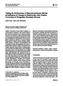
the measure relied upon for skill inference is equally sensitive to skill and effort. The incentive benefit derived from combining disparate signals of effort and skill is reflected in Proposition 1 by the fact that the higher α1 and/or lower β1 , the more likely aggregation is to be preferred. In fact, for β1 < 1 / 2, aggregation is sure to be efficiency enhancing.9 Figure 2 pictorially summarizes the potential for increased effort incentives that can accompany aggregation using four different (α1, β1 )-parameterizations. In drawing the figure, we set v(e) = e2 / 2 and δ = 1. The figure highlights that (i) α1 > β1 is a necessary condition for increased effort incentives under aggregation so, for example, when α1 = 3/5 and β1 = 2 / 3, e A < e D for any precision ratio, (ii) α1 > β1 and a large precision ratio is necessary and sufficient for aggregation to yield increased effort incentives–the precision ratio value above which e A > e D corresponds to the cutoff expression in Proposition 1, (iii) for a given β1 ( β1 = 2/3 in the figure), an increase in α1 (from 3/4 to 4/5) makes the outcomes more dissimilar and, thus, results in an increased preference for aggregation (the precision ratio cutoff declines from 4 to 2.5), and (iv) when β1 < 1 / 2, aggregation is efficiency enhancing for any precision ratio. eA -eD Ha1 =3ê5, b1 =1ê3L
Ha1 =4ê5, b1 =2ê3L
Ha1 =3ê4, b1 =2ê3L
1
2.5
4
5
te ÅÅÅÅÅÅÅÅÅ tq
Ha1 =3ê5, b1 =2ê3L
Figure 2: Effort incentives as a function of the precision ratio. 9
In the parlance of Dewatripont et al. (1999a), when the proposition conditions are satisfied, type and effort are oppositely ordered with respect to any individual measure conditional on the aggregate measure. Thus, the observation of an individual measure after having observed the aggregate measure creates perverse incentives in that marginally higher effort reduces market perception of skill.
13
While Proposition 1 addresses the circumstance in which aggregation of two output measures is optimal, the machinery used therein can readily be applied to the extended case of n output measures. In particular, say that output i, i = 1, ..., n, is qi = α iθ + β i e + ε i , where ε i ' s are independent noise terms with variance σ ε2 , and again normalize the effort n
n
i=1
i=1
and skill coefficients such that ∑ α i = ∑ β i = 1. The following corollary presents the noutput analog to Proposition 1. Corollary. In the n-output setting, the use of an aggregate performance measure yields n
greater effort incentives and thereby higher efficiency if and only if ∑ α i [α i − β i ] > 0 and i=1 ⎡ n ⎤ ⎡n ⎤ τ ε τ θ > ⎢n ∑ α iβ i − 1⎥ ⎢ ∑ α i [α i − β i ]⎥ . ⎣ i=1 ⎦ ⎣i=1 ⎦ Taken together, the results in the proposition and corollary suggest that circumstances where aggregation is most beneficial are those in which there is (i) large uncertainty (low τ θ ) about an agent's skill, (ii) little inherent measurement error (high τ ε ) in output, and/or (iii) substantial skill/effort separation in distinct output measures. n
In the n-output case, (iii) is reflected best by ∑ α iβ i . When measures that are i=1
informative of skill (higher α i ) are associated with less sensitivity to effort (lower β i ), n
n
i=1
i=1
∑ α iβ i is lower. Thus, the lower ∑ α iβ i , the greater is the skill/effort separation and the
more attractive is aggregation. As a consequence, while casual intuition may suggest that aggregation is most appropriate when the items under consideration are similar in nature, the reverse is true in providing implicit incentives: aggregation is most appealing when the items being aggregated are themselves not alike. 3.4. Aggregate Disclosure vs. Limited Disclosure While aggregation is typically deemed costly due to inherent information destruction, the preceding analysis demonstrates that information reduction can be helpful. Given this basic premise, it seems worthwhile to digress a bit to distinguish aggregation from pure information suppression. After all, as Autrey et al. (2007a) note, infusion of
14
public information, particularly about the agent's skill, can disturb implicit incentives. It is important to note, though, that while aggregation does serve to coarsen information, it does so in a particular way. That is, it not only leaves the information recipient less certain about the agent's skill, but can also make it such that the agent's effort can have a greater impact on such (weakened) inferences. Its ability to enhance effort incentives without excessive loss of information is a characteristic that can distinguish aggregation from other forms of information suppression. To see this, consider the alternative means of suppressing information in this paper's model: the removal of q1 or q2 from the public eye.10 In this case, if only qi is available to the market in determining the agent's continuation wage, the equilibrium effort level is determined as follows. ˆ the market's Again denoting the market's conjecture of the agent's effort by e, updated belief of the agent's skill, θ, given observation of only qi has a mean of ˆ = θ i (qi , e)
ˆ αi ] τ θ θ + α i 2 τ ε [(qi − β i e) . τθ + αi2τ ε
(7)
As with aggregation, the posterior mean in (7), entails a greater weight placed on the prior ˆ the than if both q1 and q2 are observed. Given the market's conjecture of agent effort, e, ˆ Holding the market's conjecture fixed, the competitive market sets wage w2 = θ i (qi , e). agent chooses effort to solve
[
]
ˆ − v(e). Max Eθ , ε i δθ i (α iθ + β i e + ε i , e) e
(8)
The first-order condition of (8) is:
δτ ε α iβ i = v ′(e). αi2τ ε + τθ
(9)
1 0 Of course, in many circumstances complete suppression of information may not even be an option. In
financial statement preparation, for example, firms have substantial discretion about the extent of aggregation in reporting, but do not have the option of excluding certain aspects of performance. Despite the frequently impractical nature of information exclusion, we undertake the comparison to highlight that aggregation is more than just an imperfect substitute for deletion of information.
15
Following the logic from before, the (unique) solution to (9) reflects the equilibrium effort level under an output report of only qi. Comparing (3), (6), and (9) then yields the following proposition. Proposition 2. An aggregate performance measure yields greater effort incentives and thereby higher efficiency than tracking either one or both of the individual measures if 2β1 − 1 τ ε 2β1 − 1 α1 and only if α1 > β1 and < < + . α1 − β1 τ θ α1 − β1 [α1 − β1 ][1 − α1 ] The lower bound on the precision ratio in Proposition 2 comes from the previous comparison of aggregation and disaggregation: for aggregation to be preferred, the measurement precision must be sufficiently high and the skill/effort dichotomy of the two measures must be sufficiently pronounced. The upper bound in the proposition comes from a comparison of aggregation with disclosure of only q2 as discussed next. With α1 > β1, q1 is more skill-sensitive while q2 is more effort-sensitive. This implies that the agent's implicit incentives to choose effort are stronger when the market learns (q1,q2) than when it learns only the skill-sensitive measure q1. After all, in the (q1,q2) case, the market puts positive weight on q2, a measure the agent can push up considerably through his effort. Thus, any time aggregation is preferred to disaggregate measures, it also dominates the regime in which only q1 is revealed. Comparing the aggregation regime with that when only q2 is observed is equivalent to contrasting the following outcome generating processes. In the aggregation case, the process is q1 + q2 = θ + e + ε1 + ε 2 .
In the single measure case, the process is
q2 / α 2 = θ + (β 2 / α 2 )e + ε 2 / α 2 . Clearly, the latter is more sensitive to effort than q1 + q2 (since β 2 / α 2 > 1). However, the single measure observation, q2 / α 2 , is more noisy than that under aggregation. The condition for aggregation to be preferred is that the error term is sufficiently noise prone that the market relies much more on the prior in the q2-case, thereby undercutting agent effort incentives. This yields the upper bound on the precision ratio in the proposition.
16
In short, aggregation represents the middle ground between full revelation of output information and the suppression of one output measure. Accordingly, aggregation is preferred for intermediate levels of performance measure precision. 3.5. Correlation in Performance Measures Inquiries about aggregation inevitably raise the issue of correlation, since one key benefit of aggregation in the presence of measurement error lies in its ability to cancel negatively correlated errors. On the other hand, if errors in measurement are positively correlated, aggregation tends to magnify the consequences of summing errors. In the preceding analysis, a subtle dichotomy arose: what is often viewed as the downside of aggregation (loss of information) can actually prove beneficial when career incentives are in view. In light of this dichotomy, we now revisit the effect of correlation on the desirability of aggregation in providing implicit incentives. In particular, consider the baseline model, except that ε1 and ε 2 have correlation
ρ ∈[−1,1]; the baseline model corresponds to the special case of ρ = 0. In this case, under disaggregation, the market's updated belief of the agent's skill, θ, given observation of q1 and q2 has a mean of ˆ ρ) = θ (q1,q2 , e; ˆ α1 ] + τ ε α 2 [α 2 − ρα1 ][(q2 − β 2e) ˆ α2 ] τ θ [1 − ρ 2 ]θ + τ ε α1[α1 − ρα 2 ][(q1 − β1e) . 2 τ θ [1 − ρ ] + τ ε α1[α1 − ρα 2 ] + τ ε α 2 [α 2 − ρα1 ]
(10)
Though the posterior mean in (10) is a bit more complicated than that in (1), it can again be cast as a weighted average of the prior of θ, an estimate of θ from q1, and an estimate of θ from q2. However, in this case, the weights depend on the extent of correlation in the measures. With positive correlation the weight on an individual output measure can even be negative, reflecting the use of one measure to cancel the measurement error in another. Also, note in the extreme case of perfect correlation (either positive or negative),
17
the posterior places all weight on the output measures (and none on the prior), reflecting the fact that the market, taking e as given, can perfectly infer θ from joint observation of the two measures. What remains to be seen is how this correlation effect translates into effort incentives. Given the market's updated belief in (10), the agent chooses effort to maximize the expected present value of his wage, less cost of effort, or
[
]
ˆ ρ ) − v(e). Max Eθ , ε1 , ε 2 δθ (α1θ + β1e + ε1, α 2θ + β 2e + ε 2 , e; e
(11)
Taking the first-order condition of (11) yields:
δτ ε [α1 (β1 − ρβ 2 ) + α 2 (β 2 − ρβ1 )] = v ′(e). [1 − ρ 2 ]τ θ + [α12 + α 22 − 2ρα1α 2 ]τ ε
(12)
Notice from (12) that if, for example, β1 is sufficiently small and ρ and α1 are sufficiently large, the use of a negative weight in (10) actually translates into a negative incentive to exert effort (in which case the agent exerts zero effort). That is, if the first (second) output measure is very sensitive to skill (effort) and the two are positively correlated, the market's use of the second primarily to cancel the error in the first means that the agent's best means of influencing perceptions is not to take effort: effort increases q2 which is indicative of high error which, for a given q1, is indicative of lower skill. Roughly stated the canceling of errors effect implies that the agent's perception of skill is increasing in q1 - q2, inducing the agent to minimize q2 via taking no effort. Such perverse incentives can be alleviated via aggregation, since it forces the market to put equal weights on the two output measures. More generally, however, depending on the particular skill and effort coefficients, correlation can also increase the agent's effort incentive. Take, for example, the case of
α1 = β1 = 1, where any non-zero correlation increases reliance on q1 because of the ability to better identify the error term ε1 via q2. This, in turn, increases the agent's incentive to
18
posture via effort. Given the ambiguous effect of correlation on effort incentives under disaggregation, we next consider its effect under aggregation. Under aggregation, the market's updated belief of the agent's skill, θ , given observation of q1 + q2 is: ˆ ρ) = θ (q1 + q2 , e;
ˆ τ θ [1 + ρ ]θ + [ τ ε / 2][q1 + q2 − e] . τ θ [1 + ρ ] + [ τ ε / 2]
(13)
From (4) and (13), the effect of correlation on the market's posterior mean is straightforward: the weight placed on the aggregate observation is decreasing in ρ, reflecting reduced diversification (and, hence reduced measurement precision) associated with adding increasingly correlated error terms. Given (13), the agent chooses effort to solve
[
]
ˆ ρ ) − v(e). Max Eθ , ε1 , ε 2 δθ (θ + e + ε1 + ε 2 , e; e
(14)
The first-order condition of (14) is:
δ [ τ ε / 2] = v ′(e). [ τ ε / 2] + τ θ [1 + ρ ]
(15)
The first-order condition in (15) reflects the view that higher correlation reduces market reliance on the aggregate measure, thereby reducing the agent's implicit incentives for effort. Comparing (12) and (15) yields the following proposition. Proposition 3. With correlation ρ , the use of an aggregate performance measure yields greater effort incentives and thereby higher efficiency if and only if α1 > β1 and τ ε [1 + ρ ][2β1 − 1] > . τθ α1 − β1 In Proposition 1, the greater the measurement precision (relative to the precision of the prior), the more appealing is aggregation. This same view carries forward in Proposition 3, where higher correlation reflects lower inherent measurement precision due to the lack of diversification when error terms are summed. While the intuitive cutoff form is consistent
19
with the view that the higher (lower) the correlation in measurement errors, the lesser (greater) the appeal of aggregation, one caveat remains. Recall from the discussion following (12) that when the spread between α1 and β1 is sufficiently large, higher correlation can severely diminish (even entirely remove) effort incentives with disaggregate information. In such circumstances, aggregation is generally preferred (from Proposition 3, the cutoff is sure to be satisfied when β1 < 1 / 2). Given this force, when aggregation is preferred, the benefit of increased effort can be more pronounced at higher values of ρ.11 As a result, while the cutoff for a preference toward aggregation is more stringent with higher correlation, one cannot unequivocally say that higher correlation always reduces the net benefit of aggregation. 3.6. Multiple Dimensions of Skill The analysis thus far considers effort incentives when the market uses observed outputs to draw inference about one aspect of an agent's skill. However, a more complete picture entails the market making inferences about different dimensions of the agent's skill set. For example, the performance of a manager's segment may speak to her judgment in hiring, ability to inspire subordinates, strategic vision, etc. Further, some of these aspects may be more clearly identified in some measures than in others. In this section, we expand the analysis to incorporate the notion that career concerns can arise with multiple dimensions of skill, and investigate the efficacy of aggregation in such cases. In particular, suppose the agent's skill set has m elements, m ≥ 1, denoted θ1, ..., θm. The (common knowledge) prior belief is that each θ j is independent and normally distributed with mean θ m and variance σ θ2 m. In this case, output i, i = 1, 2, is m
qi = ∑ α ij θ j + β i e + ε i ,
Again, the effort and skill coefficients are such that
j =1
1 1 The ambiguous effect of correlation on the net benefit of aggregation can best be seen in an example.
Say α1 = 4/5 and β1 = 1/5; by Proposition 3, aggregation is preferred for all ρ. In the case of quadratic effort cost, the increase in effort due to aggregation is increasing in ρ for ρ ∈ [-1,8/17) and decreasing in ρ for ρ ∈ (8/17,1].
20 m
m
j =1
j =1
α1j + α 2j = β1 + β 2 = 1 ∀j , and without loss of generality, let ∑ α1j > ∑ α 2j . Also, we normalize the market's assessment of ability (continuation wage) as the expected sum of the agent's skill components. In other words, this setting is one where the mean and variance of the agent's total skill are as in the baseline setup, but output measures may have different sensitivities to different aspects of skill. ˆ Under disaggregation, denoting the market's conjecture of the agent's effort by e, m
the market's updated belief of the agent's total skill, θ = ∑ θ j , given observation of q1 and j =1
q2 is normally distributed with a mean of ˆ = λ1[(q1 − β1e) ˆ α1 ] + λ 2 [(q2 − β 2e) ˆ α 2 ] + (1 − λ1 − λ 2 )θ , where θ (q1,q2 , e) ⎡ ⎛ m ⎛ m ⎞⎤ mτ θ ⎞ j 2 α i ⎢( mα i )⎜ ∑ (α −i ) + − ( mα −i )⎜ ∑ α1j α 2j ⎟ ⎥ ⎟ τε ⎠ ⎝ j =1 ⎝ j =1 ⎠ ⎥⎦ 1 m j ⎢ λi = ⎣ ∑ α i , i = 1,2. (16) 2 and α i = m m m j =1 ⎡m ⎡ ⎡ ⎤ ⎤ ⎤ mτ θ mτ θ j 2 j 2 j j ⎢ ∑ ( α1 ) + ⎥ ⎢ ∑ (α 2 ) + ⎥ − ⎢ ∑ α1 α 2 ⎥ τ ε ⎦ ⎣ j =1 τ ε ⎦ ⎣ j =1 ⎣ j =1 ⎦ The posterior mean in (16) again takes the form of a weighted average of the prior and m
estimates of ∑ θ j gleaned from each observation. In this case, the estimate of total skill j =1
gleaned from a single output measure is that measure with the impact of effort removed, scaled by the average α j -coefficient on the θ j 's. Intuitively, since the market cares about each dimension of skill equally and is unable to disentangle the coefficient on each aspect, it simply takes the average value in divining an estimate. However, in combining these individual estimates to come up with the best overall guess of agent ability, the market places different weight on each estimate reflecting their relative informativeness. For instance, if one measure is balanced (equally sensitive to each dimension of skill), the updated belief puts a greater weight on this measure than if the measure was unbalanced. As a simple example to see this role of dispersion in α j coefficients, consider the case of a single measure when σ ε2 = 0. If all α j 's are equal, the
21
market can use this balanced measure to perfectly infer the agent's total skill. In contrast, if any two α j 's are unequal, the market includes the prior for at least some guidance. Given the market's updated beliefs in (16), the agent chooses effort to solve Max Eθ 1 ,L,θ m , ε e
m m ⎤ ⎡ j j j j ˆ ⎥ − v(e). δθ θ ( α θ + β e + ε , α θ + β e + ε , e) ∑ ∑ ⎢ 1 1 2 2 1 2 1 ,ε 2 j =1 j =1 ⎣ ⎦
(17)
The first-order condition of (17) is: 2
δ ∑ [β i λ i α i ] = v ′(e).
(18)
i=1
Now, we turn to the aggregation outcome. In this case, the aggregate measure is m
m
j =1
j =1
m
q1 + q2 = ∑ α1j θ j + ∑ α 2j θ j +β1e + β 2e + ε1 + ε 2 = ∑ θ j + e + ε1 + ε 2 . Since the market m
j
j =1
wage represents a best-guess of ∑ θ , we can restate the problem in terms of the onej =1
m
dimensional skill equilibrium as in section 3.2, where θ = ∑ θ j . Thus, the agent's firstj =1
order condition for effort under aggregation is simply that in (6). Comparing (18) and (6) determines the more efficient regime. Proposition 4. In the case of m-dimensional skill, the use of an aggregate performance measure yields greater effort incentives and thereby higher efficiency if and only if τ 2β − 1 α1 > β1 and ε > 1 . τ θ α1 − β1 In the case of multiple dimensions of skill, one may naively intuit that since the market cares only about the agent's total skill and is unable to distinguish the individual components in each measure, the problem reduces to one in which the market is assessing a single component of skill with the coefficients on the one-dimensional skill equal to α1 and
α 2 in q1 and q2, respectively. That is, this view suggests that the analysis is precisely as before, except α i is replaced by α i . Of course, the underlying forces are more subtle, reflected in the fact that although market estimates from each measure follow the naive view, the market's reliance on a given estimate depends on not just α i but also the dispersion in
α ij 's as in (16).
22
It is, hence, particularly surprising that the simple cutoff in the proposition is consistent with the naive view. That is, while the net gain (or loss) from aggregation is much different than that in section 3.3, and depends on dispersion in α ij 's , the condition under which aggregation is preferred continues to have a simple interpretation. 3.7. Multiple Dimensions of Effort Just as varied facets of skill can have different effects on various performance measures, effort too can take different forms with each influencing performance measures in differing ways. This section appends the analysis to incorporate the possibility of multiple dimensions of effort to reflect the fact that an employee can target his efforts to maximize external perceptions. In particular, return to the baseline model but suppose the agent can undertake l different efforts, l ≥ 1, denoted e 1 , ..., e l . l
qi = α iθ + ∑ β ik e k + ε i .
k =1 α1 + α 2 = β1k + β 2k
In this case, output i, i = 1, 2, is
Again, the effort and skill coefficients are such that
= 1 ∀k . In this case, the agent's cost of effort is v(e1 +...+el ).
Under disaggregation, denoting the market's conjecture of the agent's efforts by eˆ = (eˆ1,..., eˆ l ) , the market's updated belief of θ, given observations of q1 and q2 is normally distributed with a mean of l l ⎡ ⎡ ⎤ ⎤ τ θ θ + α12 τ ε ⎢(q1 − ∑ β1k eˆ k ) / α1 ⎥ + α 2 2 τ ε ⎢(q2 − ∑ β 2k eˆ k ) / α 2 ⎥ k =1 k =1 ⎣ ⎣ ⎦ ⎦ . (19) ˆ = θ (q1,q2 , e) 2 2 τ θ + α1 τ ε + α 2 τ ε
The posterior mean in (19) is simply that in (1), where the estimates of θ are adjusted to reflect expectations of the various efforts. Given the market's updated beliefs in (19), the agent chooses effort to solve l l l ⎡ ⎤ k k k k ˆ Max E δθ ( α θ + β e ε , α θ + β e ε , e) + + − v( ek ) . ∑ ∑ ∑ 1 1 1 2 2 2 θ , ε1 , ε 2 ⎢ ⎥ 1 l e ,L,e k =1 k =1 k =1 ⎣ ⎦
Denoting K = argmax β1k , the first-order conditions of (20) reveal that: k
(20)
23
k
e = 0 for k ≠ K and In
the
case
of
e K solves
aggregate
δτ ε [α1β1K + α 2β1K ] = v ′(e K ). 2 2 τ ε [ α1 + α 2 ] + τ θ
measures,
the
l
l
l
k =1
k =1
k =1
observed
measure
(21) is
q1 + q2 = α1θ + α 2θ + ∑ β1k e k + ∑ β 2k e k +ε1 + ε 2 = θ + ∑ e k + ε1 + ε 2 . Since both the aggregate output and the agent's effort cost depend only on the sum of efforts, the aggregate case can be restated in terms of the one-dimensional effort problem as in section 3.2, where l
e = ∑ e k . Thus, the agent's first-order condition for (aggregate) effort under aggregation is k =1
simply that in (6). Comparing (21) and (6) determines the more efficient regime. Proposition 5. In the case of l-dimensional effort, the use of an aggregate performance measure yields greater effort incentives and thereby higher efficiency if and only if τ ε 2β1K − 1 K α1 > β1 and > . τ θ α1 − β1K Intuitively, under aggregation, the agent has no incentive to fine-tune efforts to disproportionately influence particular measures, since only the total output is observed. In contrast, under disaggregation, the agent can choose to target his effort toward that dimension which has the largest impact on market perceptions. Since α1 > 1 / 2 , the first output measure q1 is the one relied on more by the market in inferring agent skill. As one may expect, then, the agent siphons effort to the dimension which can influence that outcome most, i.e., that which has the highest β1k . The comparison between aggregation and disaggregation again amounts to asking how large is the skill-effort dichotomy under disaggregation. Since that dichotomy is influenced by the fact the agent can focus effort, the conditions under which aggregation is preferred are analogous to before except the cutoff is determined by the most prominent effort dimension. 4. Conclusion The pervasiveness of aggregate measures, particularly in the realm of employee performance indicators, has long been a puzzle due to the inherent loss of information.
24
Though the provision of incentives is generally enhanced by knowledge of disaggregated details when complete contingent incentive contracts are feasible, this paper demonstrates that such a view does not necessarily carry forward to the case of implicit career incentives. In particular, the paper shows that aggregation can enhance incentives when individual performance measures exhibit differences in terms of their sensitivities to effort and talent. In such a case, the use of an aggregate measure leads an employee to undertake effort so as to influence market perceptions of ability; on the other hand, separate measures diminish such an incentive due to the fact that the market puts primary emphasis on skill-intensive measures (and disregards those influenced by effort) in making assessments. This impetus for effort generated by aggregation is weighed against the dampened incentives that come from the inherent information loss: due to this loss, the market relies less on the aggregate measure and thus the employee feels less inclined to try to influence it. Besides demonstrating that aggregation can be preferred even in the absence of transmission and processing costs, the paper also demonstrates key determinants of such a preference. In particular, the results suggest that aggregate measures are most appealing in circumstances wherein implicit incentives play a key role, measurement error is limited, and the performance measures of interest are distinct in terms of their drivers. Further research could investigate how such forces are influenced by the presence of product market competition, team incentives, differential stages of employee careers, or the desire to better match employee skills to employer needs. Such extensions may shed light on why some firms are more willing to publicly reveal detailed (disaggregate) performance information than others or why firms may choose to provide detailed information about some operating units while providing only summary information about others.
25 APPENDIX Proof of Proposition 1. The proofs in the appendix make use of the following standard result (e.g., Greene ⎡ X1 ⎤ ⎡ µ1 ⎤ 1997, p. 90): if X = ⎢ ⎥ is multivariate normal with mean µ = ⎢ ⎥ , covariance matrix ⎣X 2 ⎦ ⎣µ 2 ⎦ ⎡ Σ11 Σ12 ⎤ Σ=⎢ ⎥ , and Σ 22 > 0, then the conditional mean of X1 , given X 2 = x 2 , is: ⎣ Σ 21 Σ 22 ⎦ −1 E(X1 x 2 ) = µ1 + Σ12 Σ 22 (x 2 − µ 2 ) .
(A1)
Step 1. In this step, we calculate the agent's effort if the market learns both q1 and q2. With disaggregate information, the agent's continuation wage, w2, is the conditional mean where ⎡ q1 ⎤ ˆ Thus, µ1 = θ and X1 = θ and X 2 = ⎢ ⎥ in (A1); this wage is denoted θ (q1,q2 , e). ⎣q2 ⎦ ⎡ α θ + β1eˆ ⎤ µ2 = ⎢ 1 ⎥ , where eˆ is the market's conjecture about the agent's effort. Also, ⎣α 2 θ + β 2eˆ ⎦ Σ12 =
[
α1σ θ2
α 2 σ θ2
] and Σ 22
ˆ =θ+ w2 = θ (q1,q2 , e)
[
α1σ θ2
⎡σ ε2 + α12 σ θ2 =⎢ 2 ⎣ α1α 2 σ θ
α 2 σ θ2
ˆ =θ+ ⇒ w2 = θ (q1,q2 , e)
α1α 2 σ θ2 ⎤ ⎥ . Using these in (A1) yields: σ ε2 + α 22 σ θ2 ⎦
⎡σ ε2 + α12 σ θ2 ⎢ 2 ⎣ α1α 2 σ θ
]
−1
α1α 2 σ θ2 ⎤ ⎛ ⎡ q1 ⎤ ⎡ α1 θ + β1eˆ ⎤⎞ −⎢ ⎥ ⎥ σ ε2 + α 22 σ θ2 ⎦ ⎜⎝ ⎢⎣q2 ⎥⎦ ⎣α 2 θ + β 2eˆ ⎦⎟⎠
⎡ q1 − α1 θ − β1eˆ ⎤ σ θ2 α α [ ] ⎢ ⎥. 1 2 ˆ σ ε2 + (α12 + α 22 )σ θ2 q − α θ − β e 2 2 ⎦ ⎣ 2
(A2)
When the agent chooses e, he accounts for the impact of his effort on w2. The agent ˆ − v(e). Using (A2), the agent's therefore chooses e to maximize Eθ , ε , ε [δθ (q1,q2 , e)] 1
2
problem is: Max e
δθ +
ˆ ⎤ ⎡ β1 (e − e) δσ θ2 − v(e). α α [ ] 1 2 ⎢ ˆ ⎥⎦ σ ε2 + (α12 + α 22 )σ θ2 ⎣β 2 (e − e)
(A3)
The first-order condition of (A3) yields the agent's equilibrium effort level:
δσ θ2 [α1β1 + α 2β 2 ] = v ′(e). σ ε2 + [α12 + α 22 ]σ θ2
(A4)
26 Step 2. In this step, we calculate the agent's effort if the market learns only q1 + q2. With aggregate information, the agent's continuation wage, w2, is the conditional mean where X1 ˆ Since the α 's and β's = θ and X 2 = q1 + q2 in (A1); this wage is denoted θ (q1 + q2 , e). 2 each sum to 1, µ1 = θ and µ 2 = θ + eˆ . Also, Σ12 = σ θ and Σ 22 = 2σ ε2 + σ θ2 . Substituting these in (A1) yields: ˆ =θ+ w2 = θ (q1 + q2 , e)
ˆ σ θ2 [q1 + q2 − θ − e] . 2 2 2σ ε + σ θ
(A5)
ˆ − v(e). The agent's problem is to chooses e to maximize Eθ , ε1 , ε 2 [δθ (q1 + q2 , e)] Using (A5), the agent solves: Max e
δθ +
ˆ δσ θ2 [e − e] − v(e). 2 2σ ε + σ θ2
(A6)
The first-order condition of (A6) yields the agent's equilibrium effort level:
δσ θ2 = v ′(e). 2σ ε2 + σ θ2
(A7)
Step 3. In this step, we compare the effort level across the two regimes. Using (A4) and (A7), aggregation yields greater effort incentives if and only if:
δσ θ2 δσ θ2 [α1β1 + α 2β 2 ] − > 0. 2σ ε2 + σ θ2 σ ε2 + [α12 + α 22 ]σ θ2
(A8)
Replacing α2 with 1-α1 and β2 with 1-β1, and simplifying, (A8) can be written as:
δσ θ2 [2α1 − 1][(α1 − β1 )σ θ2 − (2β1 − 1)σ ε2 ] > 0. [2σ ε2 + σ θ2 ][σ ε2 + ((1 − α1 )2 + α12 )σ θ2 ]
(A9)
The denominator on the left-hand-side of (A9) is positive, so the sign of the term depends on the sign of the numerator. If α1 ≤ β1, then β1 > 1/2 (recall, α1 > 1/2). In this case, the left-hand-side term is nonpositive, and so (A9) cannot be satisfied. If α1 > β1, replacing σ θ2 with 1 / τ θ and σ ε2 with 1 / τ ε in (A9), aggregation yields greater effort if and only if the precision cutoff in the proposition is satisfied. Turning to the issue of efficiency, the first-best (efficient) effort level is found by solving the equation 1 = v ′(e). Since the left-hand-side of (A7) is less than 1, and v ′′(e) > 0, it follows that effort under aggregation is less than first-best. As a consequence, when aggregation leads the agent to choose a greater effort level, it also yields higher efficiency. This completes the proof of Proposition 1.
27 Proof of the Corollary. In the disaggregation case, the only difference relative to Step 1 in the proof of ⎡ q1 ⎤ Proposition 1 is that X 2 is now the n × 1 vector ⎢⎢ M ⎥⎥ . Not surprisingly, the agent's ⎢⎣qn ⎥⎦ continuation wage, his effort choice problem, and the equilibrium effort level are analogous to (A2) - (A4). ⎡ q1 − α1 θ − β1eˆ ⎤ σ θ2 ⎢ ⎥ ˆ =θ+ 2 w2 = θ (q1,L,qn , e) M 2 2 2 [α1 L α n ]⎢ ⎥. (A10) σ ε + (α1 +L+ α n )σ θ ⎢⎣qn − α n θ − β neˆ ⎥⎦
Max e
ˆ ⎤ ⎡ β1 (e − e) δσ θ2 δθ + 2 [α1 L α n ]⎢⎢ M ⎥⎥ − v(e). σ ε + (α12 +L+ α n2 )σ θ2 ˆ ⎥⎦ ⎢⎣β n (e − e)
δσ θ2 [α1β1 +L+ α nβ n ] = v ′(e). σ ε2 + [α12 +L+ α n2 ]σ θ2
(A11)
(A12)
In the aggregation case, the counterparts to (A5) - (A7) are also straightforward: ˆ =θ+ w2 = θ (q1 +L+qn , e)
Max e
δθ +
ˆ σ θ2 [q1 +L+qn − θ − e] . nσ ε2 + σ θ2
ˆ δσ θ2 [e − e] 2 2 − v(e). nσ ε + σ θ
δσ θ2 = v ′(e). nσ ε2 + σ θ2
(A13)
(A14)
(A15)
Aggregation yields greater effort incentives (and, in which case, also higher efficiency) if and only if the left-hand-side of (A15) exceeds the left-hand-side of (A12). Replacing σ θ2 with 1 / τ θ , and σ ε2 with 1 / τ ε , the left-hand-side of (A15) less that of (A12) is greater than 0 if and only if: n ⎡ n ⎤ τ ε ∑ α i [α i − β i ] − τ θ ⎢n ∑ α iβ i − 1⎥ > 0 . i=1 ⎣ i=1 ⎦
(A16)
28 n
n
n
If ∑ α i [α i − β i ] ≤ 0 , then ∑ α iβ i ≥ ∑ α i2 ≥ 1 / n ; the last inequality holds because n n i=1 i=1 i=1 the minimum value of ∑ α i2 occurs when α i = 1 / n. Thus, in this case, n ∑ α iβ i − 1 ≥ 0. i=1 i=1 This implies the left-hand-side of (A16) is nonpositive, and so (A16) can not be satisfied. If n
∑ α i [α i − β i ] > 0 , then (A16) is satisfied if and only if the precision ratio is above the i=1 cutoff identified in the Corollary. This completes the proof of the Corollary. Proof of Proposition 2. When the market learns only q1, the agent's continuation wage, w2, is the conditional ˆ . Thus, µ1 = θ , mean with X1 = θ and X 2 = q1 in (A1); this wage is denoted θ1 (q1, e) 2 2 2 2 µ 2 = α1 θ + β1eˆ , Σ12 = α1σ θ and Σ 22 = σ ε + α1 σ θ . Substituting these in (A1) yields w2 and, using this w 2-value, the agent's problem is formulated and solved using the same procedure as in the proof of Proposition 1. The w2-value, the agent's problem, and the equilibrium effort level are as in (A17) - (A19), respectively: ˆ =θ+ w2 = θ1 (q1, e)
Max e
δθ +
ˆ σ θ2 α1[q1 − α1 θ − β1e] . 2 2 2 σ ε + α1 σ θ
ˆ δσ θ2 α1β1[e − e] − v(e). 2 2 2 σ ε + α1 σ θ
δσ θ2 α1β1 = v ′(e). σ ε2 + α12 σ θ2
(A17)
(A18)
(A19)
From (A7) and (A19), revealing q1+q2 yields greater effort incentives than revealing only q1 if and only if:
δσ θ2 δσ θ2 α1β1 − > 0. 2σ ε2 + σ θ2 σ ε2 + α12 σ θ2
(A20)
Simplifying, when α1 > β1 (A20) is equivalent to the condition:
σ θ2 2α1β1 − 1 2β − 1 1 − α1 = 1 − . 2 > σ ε α1 (α1 − β1 ) α1 − β1 α1 (α1 − β1 )
(A21)
Comparing the variance cutoff in (A21) with that in Proposition 1, it follows that if effort incentives under q1 + q2 are greater than under (q1,q2), they are also greater than if only q1 is revealed. Replacing α1 with α2 and β1 with β2 in (A20) provides the necessary and sufficient condition for when revealing q1+q2 yields greater effort incentives than revealing only q2:
29
δσ θ2 δσ θ2 α 2β 2 − > 0. 2σ ε2 + σ θ2 σ ε2 + α 22 σ θ2
(A22)
Replacing α 2 with 1-α 1, β2 with 1-β1, σ θ2 with 1 / τ θ , σ ε2 with 1 / τ ε , and simplifying, when α1 > β1 (A22) is equivalent to:
τε 2 α 2β 2 − 1 2β − 1 α1 < = 1 + . τ θ α 2 (α 2 − β 2 ) α1 − β1 (α1 − β1 )(1 − α1 )
(A23)
Combining (A23) with the condition in Proposition 1 completes the proof of Proposition 2. Proof of Proposition 3. With correlated error terms, the analysis proceeds as in the proof of Proposition 1 except that Σ 22 is changed to account for the error correlation ρ . In particular, with ⎡ σ ε2 + α12 σ θ2 ρσ ε2 + α1α 2 σ θ2 ⎤ disaggregate outcomes (q1,q2), Σ 22 = ⎢ 2 ⎥ ; with aggregate 2 σ ε2 + α 22 σ θ2 ⎦ ⎣ρσ ε + α1α 2 σ θ outcome q1+q2, Σ 22 = 2(1 + ρ )σ ε2 + σ θ2 . With the above changes, the agent's equilibrium effort under (q1,q2), if interior, solves the following first-order condition:
δσ θ2 [α1 (β1 − ρβ 2 ) + α 2 (β 2 − ρβ1 )] = v ′(e). [1 − ρ 2 ]σ ε2 + [α12 + α 22 − 2ρα1α 2 ]σ θ2
(A24)
(A24) is the counterpart to (A4); in addition, if the left-hand-side of (A24) is negative, the agent's effort is 0. The agent's equilibrium effort under q1+q2, the counterpart to (A7), is obtained by solving:
δσ θ2 = v ′(e). 2(1 + ρ )σ ε2 + σ θ2
(A25)
Notice the left-hand-side of (A25) is positive, so the agent's effort is greater than 0. Thus, using (A24) and (A25), aggregation yields greater effort incentives (and, in which case, also higher efficiency) if and only if:
δσ θ2 δσ θ2 [α1 (β1 − ρβ 2 ) + α 2 (β 2 − ρβ1 )] − > 0. 2(1 + ρ )σ ε2 + σ θ2 [1 − ρ 2 ]σ ε2 + [α12 + α 22 − 2ρα1α 2 ]σ θ2
(A26)
Replacing α 2 with 1-α 1 , β 2 with 1-β 1 , σ θ2 with 1 / τ θ , σ ε2 with 1 / τ ε , and simplifying, (A26) holds if and only if:
30 [2α1 − 1][(α1 − β1 )τ ε − (1 + ρ )(2β1 − 1)τ θ ] > 0.
(A27)
(A27) holds if and only if the condition in Proposition 3 is satisfied, thus completing the proof of the proposition. Proof of Proposition 4. ⎡ q1 ⎤ Under disaggregation, X1 = θ 1 +...+θ m and X 2 = ⎢ ⎥ in (A1). Thus, µ1 = θ and ⎣q2 ⎦ m ⎤ ⎡ ( θ / m) α1j + β1eˆ ⎥ ∑ ⎢ m m ⎡ 2 ⎤ j =1 j 2 ⎥ , Σ ( and µ2 = ⎢ = ( σ / m) α σ / m) α 2j ⎥ , ∑ ∑ ⎢ θ 12 θ 1 m j =1 j =1 ⎦ ⎢(θ / m) ∑ α j + β eˆ ⎥ ⎣ 2 2 ⎢⎣ ⎥⎦ j =1 m m ⎤ ⎡ 2 j 2 2 2 ( σ + ( σ / m) ( α ) σ / m) α1j α 2j ⎥ ∑ ∑ ε θ θ 1 ⎢ j =1 j =1 ⎥ . Using the same arguments as Σ 22 = ⎢ m m j 2⎥ 2 2 ⎢ (σ 2 / m) ∑ α j α j σ + ( σ / m) ( α ) ∑ 2 ε θ θ 1 2 ⎢⎣ ⎥⎦ j =1 j =1 before, some tedious calculations confirm that the agent's equilibrium effort under (q1,q2), the counterpart to (A4), solves: 2 ⎡⎛ m j ⎞ ⎛ m mσ 2 ⎞ ⎛ m j ⎞ ⎛ m j j ⎞ ⎤ j 2 ∑ δβ i ⎢⎜ ∑ α i ⎟ ⎜ ∑ (α −i ) + 2ε ⎟ − ⎜ ∑ α −i ⎟ ⎜ ∑ α1 α 2 ⎟ ⎥ σ θ ⎠ ⎝ j =1 ⎠ ⎝ j =1 ⎠ ⎥⎦ i=1 ⎢⎣⎝ j =1 ⎠ ⎝ j =1 = v ′(e). 2 2 ⎤⎡ m 2⎤ ⎡ m ⎡m ⎤ m m σ σ j 2 j 2 j j ε ε ⎢ ∑ ( α1 ) + 2 ⎥ ⎢ ∑ ( α 2 ) + 2 ⎥ − ⎢ ∑ α1 α 2 ⎥ σ θ ⎦ ⎣ j =1 σ θ ⎦ ⎣ j =1 ⎣ j =1 ⎦
(A28)
The agent's effort under q1 + q2 is, of course, as in (A7). Thus, aggregation yields greater effort incentives (and, in which case, also higher efficiency) if and only if the lefthand-side of (A7) exceeds the left-hand-side of (A28). Replacing α 2j with 1 − α1j , β2 with 1-β1, σ θ2 with 1 / τ θ , and σ ε2 with 1 / τ ε , the left-hand-side of (A7) less that in (A28) is greater than 0 if and only if: m
[2α1 − 1][(α1 − β1 )τ ε − (2β1 − 1)τ θ ] > 0 , where α1 = ∑ α1j / m.
(A29)
j =1
(A29) holds if and only if the condition in Proposition 4 is satisfied, thus completing the proof of the proposition.
31 Proof of Proposition 5. ⎡ q1 ⎤ Under disaggregation, X1 = θ and X 2 = ⎢ ⎥ in (A1). Thus, µ1 = θ and ⎣q2 ⎦ l ⎤ ⎡ α θ + β1k eˆ k ⎥ ∑ 1 ⎢ ⎡σ ε2 + α12 σ θ2 α1α 2 σ θ2 ⎤ 2 2 k =1 , Σ . µ2 = ⎢ ⎥ 12 = α1σ θ α 2 σ θ , and Σ 22 = ⎢ l 2 2⎥ 2 2 k k α α σ σ + α σ ⎢α 2 θ + ∑ β 2 eˆ ⎥ ε 2 θ⎦ ⎣ 1 2 θ ⎢⎣ ⎥⎦ k =1 Using these in (A1) yields: l ⎤ ⎡ q − α θ − β1k eˆ k ⎥ ∑ 2 1 1 ⎢ σθ k =1 ˆ =θ+ 2 w2 = θ (q1,q2 , e) ⎥. (A30) [α1 α 2 ]⎢ l σ ε + (α12 + α 22 )σ θ2 ⎢q2 − α 2 θ − ∑ β 2k eˆ k ⎥ ⎢⎣ ⎥⎦ k =1
[
]
Using (A30), the agent's problem is: Max
e1 ,L,e l
δθ +
δσ θ2 σ ε2 + (α12 + α 22 )σ θ2
[ α1
⎡ l k k ˆk ⎤ l ⎢ ∑ β1 (e − e )⎥ − v( e k ). α 2 ]⎢k =1 ∑ ⎥ l k =1 ⎢ ∑ β 2k (e k − eˆ k )⎥ ⎢⎣k =1 ⎥⎦
(A31)
Since the agent's cost of effort depends only on total effort, from (A31) it follows that the agent chooses one nonzero effort dimension, e K , where K is the k-value that maximizes α1β1k + α 2β 2k = α1β1k + (1 − α1 )(1 − β1k ) . Using (A31), eK solves: Max K e
Since α1 > 1 / 2 , K = argmax β1k .
⎡β1K (e K − eˆ K )⎤ δσ θ2 K δθ + 2 ⎥ − v(e ). 2 2 2 [α1 α 2 ]⎢ K K K σ ε + ( α1 + α 2 )σ θ ⎣β 2 (e − eˆ )⎦
k
(A32)
The first-order condition of (A32) yields the agent's (only) nonzero equilibrium effort level:
δσ θ2 [α1β1K + α 2β 2K ] K 2 2 2 2 = v ′(e ). σ ε + [α1 + α 2 ]σ θ
(A33)
With aggregate information, X1 = θ and X 2 = q1 + q2 in (A1). Thus, µ1 = θ and l µ 2 = θ + ∑ eˆ k , Σ12 = σ θ2 , and Σ 22 = 2σ ε2 + σ θ2 . Substituting these in (A1) yields: k =1
l ⎡ ⎤ σ θ2 ⎢q1 + q2 − θ − ∑ eˆ k ⎥ k =1 ⎦ ⎣ ˆ =θ+ w2 = θ (q1 + q2 , e) . 2 2 2σ ε + σ θ
Using (A34), the agent solves:
(A34)
32 Max
e1 ,L,e l
⎡ l ⎤ δσ θ2 ⎢ ∑ (e k − eˆ k )⎥ ⎣k =1 ⎦ − v( l e k ). δθ + ∑ 2 2 2σ ε + σ θ k =1
(A35)
l
From (A35), there is a unique solution to ∑ e k ; how the agent chooses each individual ek is k =1
immaterial. The first-order condition of (A35) yields the equilibrium total effort: l δσ θ2 v ( e k ). = ′ ∑ 2 2 2σ ε + σ θ k =1
(A36)
From (A33) and (A36), the total effort is higher under aggregation if and only if
δσ θ2 δσ θ2 [α1β1K + α 2β 2K ] − > 0. 2σ ε2 + σ θ2 σ ε2 + [α12 + α 22 ]σ θ2
(A37)
Notice (A37) is the same as (A8) but for the fact that β i is replaced with β iK . Thus, but for this β-change, the result is the same as in Proposition 1.
33 References Akerlof, R. and R. Holden. 2005. Ignorance is bliss? Why firms may not want to monitor their workers. Working Paper, Harvard University. Auriol, E., G. Friebel and L. Pechlivanos. 2002. Career concerns in teams. Journal of Labor Economics 20: 289–307. Autrey, R., S. Dikolli and P. Newman. 2007a. Career concerns and mandated disclosure. Journal of Accounting and Public Policy 26: 527-554. Autrey, R., S. Dikolli and P. Newman. 2007b. Mitigating agency costs due to performance measure aggregation: The role of career incentives. Working Paper, Duke University. Demski, J. and H. Frimor. 1999. Performance measure garbling under renegotiation in multi-period agencies. Journal of Accounting Research 37: 187-214. Dewatripont, M., I. Jewitt, and J. Tirole. 1999a. The economics of career concerns, Part 1: Comparing information structures. Review of Economic Studies 66: 183-198. Dewatripont, M., I. Jewitt, and J. Tirole. 1999b. The economics of career concerns, Part 2: Application to missions and accountability of government agencies. Review of Economic Studies 66: 199-217. Feltham, G., R. Indjejikian, and D. Nanda. 2006. Dynamic incentives and dual-purpose accounting. Journal of Accounting and Economics 42: 417-437. Fudenberg, D. and J. Tirole. 1990. Moral hazard and renegotiation in agency contracts. Econometrica 58: 1279-1320. Gibbons, R. and K. Murphy. 1992. Optimal incentive contracts in the presence of career concerns: Theory and evidence. Journal of Political Economy 100: 468-593. Gigler, F. and T. Hemmer. 2002. Information costs and benefits of creating separately identifiable operating segments. Journal of Accounting and Economics 33: 69-90.
34 Greene, S. 1997. Econometric Analysis. Upper Saddle River, NJ: Prentice Hall. Holmstrom, B. 1982. Managerial incentives–A dynamic perspective, in Essays in Economics and Management in Honor of Lars Wahlbeck. Helsinki, Finland: Swedish School of Economics. Holmstrom, B. 1999. Managerial incentive problems: A dynamic perspective. Review of Economic Studies 66: 169-182. Holmstrom, B. and J. Ricart i Costa. 1986. Managerial incentives and capital management. Quarterly Journal of Economics 101: 835-860. Kaarboe, O. and T. Olsen. 2006. Career concerns, monetary incentives, and job design. Scandinavian Journal of Economics 108: 299-316. Meyer, M. and J. Vickers. 1997. Performance comparisons and dynamic incentives. Journal of Political Economy 105: 547-581. Milbourn, T., R. Shockley, and A. Thakor. 2001. Managerial career concerns and investments in information. RAND Journal of Economics 32: 334-351. Salanie, B. 1997. The Economics of Contracts: A Primer. Cambridge, MA: The MIT Press.