Journal of mathematics and computer Science
12 (2014) 1 - 11
The Biennial Malmquist Index in the of Negative Data Narjes Mohammadi1, Alireza Yousefpour*, 2 1. Science and Research branch, Islamic Azad university, Mazandaran, Iran. 2. Department of IT & Computer, Islamic Azad University of Qaemshahr branch, Iran
[email protected] Article history: Received May 2014 Accepted June 2014 Available online July 2014
Abstract We purpose the range directional model (RDM), a particular case of the directional distance function, is used for computing efficiency in the presence of negative data. We use RDM efficiency measures to arrive at a Malmquist-type index which can reflect productivity change. We illustrate how the biennial Malmquist index can be used, not only for comparing the performance of a unit in two time periods, but also for comparing the performance of two different units at the same or different time periods. The proposed approach is then applied to a sample of bank branches where negative data were involved. In this paper, we introduce a biennial Malmquist index of productivity change that can be used with negative data.
1. Introduction The computation of productivity change by means of efficiency measures was introduced by Caves et al. (1982) at the first time and developed by Nishimizu and Page (1982) and by Fare et al. (1994), in the context of parametric and non-parametric efficiency measurement, respectively. The Fare et al. (1994) approach has become known as the measurement of productivity change through Malmquist indices. Though several applications of Malmquist indices exist in the literature, to the authors’ knowledge there is none where efficiency measures were computed for situations where some data were negative. Negative data may arise due to the use of input–output variables like changes in clients or accounts from one period to the next in the case of our bank branches, or due to the use of variables like profit that may take both positive and negative values.
1
N. Mohammadi, A. Yousefpour / J. Math. Computer Sci. 12 (2014) 1 - 11 The use of profit measures is very common in the banking literature in particular for measuring profit efficiency. To measure efficiency under negative data we use the approach developed by Portela et al. (2004) named range directional model (RDM). To calculate Malmquist indices using the RDM we adapt the Global Malmquist index of Pastor and Lovell (2005), analyzed and extended in Portela and Thanassoulis (2008). The index uses a single reference frontier drawn on a pooled panel of data. We refer to our productivity index as the biennial Malmquist index since the frontier of a pooled panel is often referred to as a biennial frontier. We use the biennial Malmquist index not only to assess the change in the productivity of a unit over time but to also compare the productivities of two units operating at the same or different points in time. The biennial Malmquist productivity index that has three attractive features: it avoids linear programming infeasibilities under variable returns to scale, it allows for technical regress, and it does not need to be recomputed when a new time period is added to the data set.
2. DEA Malmquist productivity index Fare et al. (1992) construct the DEA-based Malmquist productivity index as the geometric mean of two Malmquist productivity indexes of Caves et al. (1982), which are defined by a distance Function D(.). Caves et al. (1982) assume D K ( x k , y k ) 1 , that is, they assume the technology for firm k is efficient, and their distance function does not reveal inefficiency. By allowing for inefficiency and modeling the technology frontier as piecewise linear, Fare et al. (1992) decompose their Malmquist productivity index into two components, one measuring the change in efficiency and the other measuring the change in the frontier technology. The frontier technology determined by the efficient frontier is estimated using DEA for a set of DMUs. However, the frontier technology for a particular DMU under evaluation is only represented by a section of the DEA frontier or a facet. Suppose we have a production function in time period t as well as period t+1. Malmquist index calculation requires two single period and two mixed period measures. The two single period measures can be obtained by using the CCR DEA model.
Dt ( xt , y t ) min n
s.t
x j 1
t i ij
n
y j 1
i
t rj
xiot , i 1, ... , n y rot , r 1, ... , s
j 0,
j 1, ... , n
t Where xiot is the ith input and y ro is the rth output for DMU in time period t. The efficiency
( Do ( xo , yo ) o ) determines the amount by which observed inputs can be proportionally reduced, t
t
t
while still producing the given output level. Using t+1 instead of t for the above model, we get t 1
t 1
t 1
( Do ( xo , y o ) , the technical efficiency score for DMU in time period t+1. t
The first of the mixed period measures, which is defined as ( Do ( xo
t 1
t 1
, y o ) for each DMU o ,
o Q{1,2,..., n}, is computed as the optimal value to the following linear programming problem:
2
N. Mohammadi, A. Yousefpour / J. Math. Computer Sci. 12 (2014) 1 - 11
min n
x
s.t
t i ij
j 1
xiot 1 , i 1, ... , n
n
y j 1
i
t rj
yrot 1 , r 1, ... , s
j 0,
j 1, ... , n t 1
t
t
Similarly, the other mixed period measure, Do ( xo , yo ) , which is needed in the computation of the output-oriented Malmquist productivity index, is the optimal value to the following linear problem:
min n
s.t
x j 1
i
n
y j 1
i
t 1 ij
xiot 1 , i 1, ... , n
t 1 rj
y rot 1 , r 1, ... , s
j 0,
j 1, ... , n
Fare et al, (1992) input-oriented Malmquist productivity index, which measures the productive change of a particular DMU o , o Q{1,2,..., n}, in time t+1 and t is given as M
Dt ( xt 1 , yt 1 ) Dt 1 ( xt 1 , yt 1 ) . Dt ( xt , yt ) Dt 1 ( xt , yt )
It can be seen that the above measure actually is the geometric mean of two Caves et al. (1982) Malmquist productivity indexes. Thus, following Caves et al. (1982) suit, Fare et al. (1992) defined that M O >1 indicates productivity gain; M O 2), a series of u-1 overlapping biennial technologies exists for each pairwise comparison of adjacent time periods. The biennial Malmquist index is defined specifically for the adjacent time periods t and t+1 since two adjacent time periods are sufficient to establish the desirable properties of avoiding infeasibility, allowing technical regress, and maintaining previous productivity calculations. Sufficiency of two time periods for these desirable properties does not preclude the construction of a triennial Malmquist index. However the biennial Malmquist index is not transitive because it is constructed from a series of overlapping two period technologies, and these technologies can differ. This drawback, however, is not uncommon; it is shared by all Malmquist indices except the global index, which is transitive because it contains a single technology. Based on the classic CRS output distance function for (x, y) defined on the period t technology, Dct ( x, y ) min{Q 0 | ( x, y ) Tct } the standard output-oriented adjacent period t Malmquist index for Q
producer j is given by t c
t j
t j
t 1 j
M (x , y , x , y
t 1 j
)
Dct ( x tj1 , y tj1 ) Dct ( x tj , y tj )
(4)
And the adjacent period t+1 Malmquist index is defined similarly, using the output distance function defined on the technology for period t+1, Dct 1 , M ct 1 likely differs from M ct , which leads to the definition of the adjacent Malmquist productivity index, M c , as the geometric mean of M ct and M ct 1 : 1
M ct ( x tj , y tj , x tj1, y tj1 ) 2 Mc ( ) M ct 1 ( x tj , y tj , x tj1, y tj1 )
(5)
i.e. similarly to the definition of Dct , wedefine the biennial output distance function D cB , based on TcB instead of T ct , i.e. Dct ( x, y ) min{Q 0 | ( x, y ) Tct } . We further define the biennial CRS Q Malmquist index for producer j as DcB ( x tj1 , y tj1 ) (6) M cB ( x tj , y tj , x tj1 , y tj1 ) DcB ( x tj , y tj )
6
N. Mohammadi, A. Yousefpour / J. Math. Computer Sci. 12 (2014) 1 - 11 Since we are using the biennial CRS technology, which includes both the period t and period t+1 technologies, we do not need to resort to any geometric mean when defining (6). The CRS benchmark technologies should be distinguished from the best practice technologies allowing for variable returns to scale (VRS). This convention enables it [the Malmquist index] to incorporate the influence of scale economies as a departure of the best practice technology from the benchmark technology. To define VRS counterparts of the CRS constructs above, consider first the period t VRS technology defined as n n Tvt ( X , Y ) X t j X t j , Y t j Y t j , t j 1 , j 1, ... , n j 1 j 1
There is only difference between Tct and Tcv that the latter includes the convexity constraint on the lambdas. Similarly the remaining VRS technologies are easily defined and denoted by the subscript “v” rather than “c”. Hence the adjacent VRS Malmquist index is given by Mv (
M vt ( x tj , y tj , x tj1, y tj1 ) M vt 1 ( x tj , y tj , x tj1, y tj1 )
1 2
)
(7)
And the biennial VRS Malmquist index is defined by B v
t j
t j
t 1 j
M (x , y , x , y
t 1 j
)
DvB ( x tj1 , y tj1 ) DvB ( x tj , y tj )
(8)
Fig.1 Illustration of the biennial Malmquist index
In Fig.1 consider two period specific frontiers (t and t+1) and a biennial-frontier (lying above the period t and t+1 frontiers for ease of illustration). Branch F observed in period t has a RDM efficiency of IF/IF when it is assessed in relation to the period t frontier. We can also assess the efficiency of branch F in relation to the biennial meta-frontier, which we refer to as biennial efficiency. The biennial efficiency of branch F is given by IF''/IF, and it can be decomposed into two components: The within-period-efficiency (IF'/IF) and a technological gap(IF''/IF'). That is, IF IF IF IF IF IF . The within-period-efficiency measures how distant the production unit is from the frontier of the period in which it was observed. The technological gap (TG) measures the distance between the period t frontier and the biennial frontier, at the input/output mix of the unit concerned.
7
N. Mohammadi, A. Yousefpour / J. Math. Computer Sci. 12 (2014) 1 - 11
Generalising, let DR t ( x tj , y tj , 0 , R y t ) (defined in (2)) be expressed as DR Bf ( x tj , y tj , 0 , R yBft ) when j
j
the technology used for computing the directional distance function of DMU j in period t is the biennial frontier. The superscript Bf on DR indicates the distance function is in relation to the metafrontier, while the superscript Bf on R indicates that the ideal point for computing the range R is a global ideal point defined over the biennial period. Thus the ideal point I r max t {max j { y rjt } , for each output (r=1,..,s). We define RDM Bf ( x tj , y tj , 0 , R yBft ) 1 DR Bf ( x tj , y tj , 0 , R yBft ) as the RDM j
output
‘biennial
efficiency’
j
unit j in period t. Further, let t t t t t t Bf Bf be the RDM ‘withinperiod-efficiency’ of unit j observed RDM ( x j , y j , 0 , R y ) 1 DR ( x j , y j , 0 , R y ) t j
of t j
in period t and computed using model (3) with technology of period t and with reference to the global ideal point defined above (Note that the within-period-efficiency is computed with reference to a global ideal point rather than to a within period ideal point, and in that respect it cannot be considered as a ‘pure’ within period measure. Retaining the same ideal point for within-period efficiencies and for biennial efficiencies makes the vector that departs from the observed point to the global ideal point collinear with the vector that departs from the target (on the within-period frontier) to the ideal point. This collinearity allows the meaningful computation of ratios between the various RDM efficiency measures as is now explained. Thus, we have:
RDM Bf ( x tj , y tj , 0 , R yBft ) RDM t ( x tj , y tj , 0 , R yBft ) TG tj j
(9)
j
Is retrieved residually as
TG Jt RDM Bf ( x tj , y tj , 0 , R yBft ) / RDM t ( x tj , y tj , 0 , R yBft ) j
(10)
j
Using the above definitions where efficiency measures are computed through the RDM model, we can define a biennial Malmquist index as: RDM Bf ( x tj1 , y tj1 , , R yBft 1 ) j (11) BM tj,t 1 RDM Bf ( x tj , y tj , , R yBft ) j
When BM tj,t 1 is greater than 1, the productivity of unit j has improved from t to t+1 (since its biennial efficiency in period t+1 is higher than that in t). Productivity has declined when BM tj,t 1 is below 1. In BM tj,t 1 we used two subsequent periods (t and t+1), but the definitions in (11) and throughout the paper are valid whatever the two periods being compared. Using (9) we can decompose the biennial Malmquist index as shown in (12).
BM tj,t 1
RDM Bf ( x tj1 , y tj1 , , R yBft 1 ) RDM t 1 ( x tj1 , y tj1 , , R yBft 1 ) TG tj1 j j Bf t t t t t Bf Bf TG tj RDM ( x j , y j , , R y t ) RDM ( x j , y j , , R y t ) j
(12)
j
The first term in (12) captures the pure technical efficiency change of unit j from year t to year t+1.
8
N. Mohammadi, A. Yousefpour / J. Math. Computer Sci. 12 (2014) 1 - 11
5. Empirical application to bank branches We consider input and output five bank branches in period t and period t+1 and to use biennial Malmquist in the model RDM to arrive at efficiency measure input and output in period t and period t+1. Bank
Input 1
Input 2
Input 3
Output 1
Output 2
Output 3
A
56.9.56
52.45
56661
3668
838983
89.453
B
5..6.95
54.51
62.7
18..3488
29225642
283428
C
975...
5..55
5..76.69
288348
83826242
588485
D
619.74
51.99
946..1
.868
692882
238842.
E
4.64.6
55.5.
5924.
.8.3488
923383488
932488
Table 1 input and output five bank branches in period t Bank
Input 1
Input 2
Input 3
Output 1
Output 2
Output 3
A
51.4.94
5..2
566.2
3238
829328
88.848
B
5.59.16
54.52
6192..1
8838433
295532439
3.2425
C
962.94
5...5
5.166.9
289346
83329245
8538492
D
6...6
51.71
77...1
833.
63.23849
8.38468
E
41.2.66
55..7
592.5.7.
.3.849
95328349
28359462
Table 2 input and output five bank branches in period t+1 t t R To using the data and this model g yrkt Ryrkt max j { yrj } yrk , r 1, .., s Calculations value yrkt for period t and period t+1.
RX11 RX12 RX13 RX21 RX22 RX23 RX31 RX32 RX33 RX41 RX42 RX43 RX51 RX52 RX53
Period t
Period t+1
0.0 447.699 1477.76 6212.77 493440.3 1104.62 7424.7 449075.9 900.35 4300.0 0.0 0.0 4422.67 80398.67 1251.51
0.0 388910.5 12571.47 5419.12 444882.45 12053.88 7343.4 396631.6 9993.16 4818.0 0.0 10492.05 46585.0 14655.0 0.0
Table 3 value R y t for period t and period t+1 rk
9
N. Mohammadi, A. Yousefpour / J. Math. Computer Sci. 12 (2014) 1 - 11 Table 4 shows optimal values t and t 1 is given by model RDM.
1 2 3 4 5
Max t
Max t 1
0.586310 0.0 0.643240 0.0 0.217417
0.0 0.1312528 0.0 0.0 0.0
Table 4 optimal values t and t 1 The solution to model RDM provides an efficiency measure is as in: RDM t ( xkt , ykt , 0 , Ry t ) 1 DRt ( xkt , ykt , 0 , Ry t ) 1 k k
k
A measure of productivity is given by the ratio of efficiency measure in two periods (t and t+1), we can define a biennial Malmquist index as: RDM Bf ( x tj1 , y tj1 , , R yBft 1 ) 1 tj 1 j BM tj,t 1 1 tj RDM Bf ( x tj , y tj , , R yBft ) j
1 0 1 2.41726896 1 0.586310 0.41369 1 0.1312528 0.8687472 BM 2t ,t 1 0.8687472 1 0 1 1 0 1 BM 3t ,t 1 2.8030048 1 0.643240 0.35676
BM 1t ,t 1
1 0 1 1 1 0 1 1 0 1 1.27293996 1 0.2174417 0.785583
BM 4t ,t 1
BM 5t ,t 1
When BM tj,t 1 is greater than 1, the productivity of unit j has improved from t to t + 1 (since its biennial efficiency in period t+1 is higher than that in t). Productivity has declined when BM tj,t 1 is below 1. DMU1 productivity has improved in period t and period t+1. DMU2 productivity has declined in period t and period t+1. DMU3 productivity has improved in period t and period t+1. DMU4 productivity has not changed in period t and period t+1. DMU5 productivity has improved in period t and period t+1.
6- Conclusion This paper has presented an approach for computing biennial Malmquist indices for measuring productivity change over time and productivity differences between units in multi-input/multi-output contexts where some of those inputs and/or outputs take negative values. The paper also shows how biennial Malmquist indices can be computed in order to compare units on performance over time. This can be useful in several contexts where a company or government body needs to monitor comparative productivity changes between units. The paper uses unit-specific
10
N. Mohammadi, A. Yousefpour / J. Math. Computer Sci. 12 (2014) 1 - 11 boundaries and the biennial-frontier to compare units on productivity, and decompose the resulting measure into a number of components capturing the position of a unit within its own unit-specific frontier and the differences in unit-specific frontiers relative to the biennial-frontier.
References [ 1 ] DW. Caves, LR. Christensen, WE. Diewert, The economic theory of index numbers and the measurement of inputs, outputs and productivity (1982). [ 2 ] R.G. Chambers, Y. Chung, R. Fare, Benefit and distance functions (1996). [ 3 ] R.G. Chambers, Y. Chung, R. Fare, Profit, directional distance functions, and Nerlovian efficiency (1998). [ 4 ] R. Färe, S. Grosskopf, M. Norris, Z. Zhang, Productivity growth, technical progress, and efficiency change in industrialized countries (1994). [ 5 ] R. Fare, S. Grosskopf, F. Hernadez-Sancho, Environmental performance: An index number approach. Resource and Energy Economics 26, 343–352 (2004). [ 6 ] M. Nishimizu, J.M. Page, Total factor productivity growth, technological progress and efficiency change (1982). [ 7 ] K.H. Park, , W.L. Weber, A note on efficiency and productivity growth in the Korean banking industry, 1992–2002, Journal of Banking and Finance 30, 2371–2386 (2006). [ 8 ] J.T. Pastor, C.A.K. Lovell, A global Malmquist productivity index. Economics Letters 88, 266– 271 (2005). [ 9 ] J.T. Pastor, C.A.K. Lovell, the biennial Malmquist productivity change index (2011). [ 10 ] M.C.A.S. Portela, E. Thanassoulis, G.P.M. Simpson, Negative data in DEA: A directional distance approach applied to bank branches. Journal of the Operational Research Society 55, 1111–1121 (2004). [ 11] M.C.A.S. Portela, E. Thanassoulis, Comparative efficiency analysis of Portuguese bank branches. European Journal of Operational Research 177, 1275–1288 (2007). [ 12 ] M.C.A.S. Portela, E. Thanassoulis, A circular Malmquist-type index for measuring productivity. AstonWorking Paper RP08-02., Aston University Birmingham B4 7ET, U (2008).
11