The Buffer Size vs. Link Bandwidth Tradeoff in Lossless Networks Alexander Shpiner
Eitan Zahavi
Ori Rottenstreich
Mellanox Technologies
[email protected]
Mellanox Technologies and Technion
[email protected]
Mellanox Technologies
[email protected]
Abstract—Data center networks demand high bandwidth switches. These networks also sustain common incast scenarios, which require large switch buffers. Therefore, network and switch designers encounter a buffer-bandwidth tradeoff as follows. Large switch buffers allow absorbing larger incast workload. However, higher switch bandwidth allows both faster buffer draining and more link pausing, which reduces buffering demand for incast. As the two features compete for silicon resources and device power budget, modeling their relative impact on the network is critical. In this work our aim is to evaluate this buffer-bandwidth tradeoff. We analyze the worst case incast scenario in the lossless network and find by how much the buffer size can be reduced, while the link bandwidth increased to stand in the same network performance. In addition, we analyze the multi-level incast cascade and support our findings by simulations. Our analysis shows that increasing bandwidth allows reducing the buffering demand by at least the same ratio, while preserving the same network performance. In particular, we show that the switch buffers can be omitted if the links bandwidth is doubled.
I. I NTRODUCTION A. Background As the popularity of cloud and high-performance computing grows, the data center networks demand higher bandwidth devices. In addition, large buffering in the switches is also required in order to sustain the temporary network oversubscription under high load. Conventional lossy networks deal with insufficient buffer sizes by dropping packets, thus bring TCP incast throughput collapse problem, which has been analyzed deeply in the recent literature [1]–[6]. A latest trend in data center networking is to use the Converged Enhanced Ethernet (CEE), whose key feature is the losslessness of the network [7]. Lossless networks do not drop packets, but use Priority Flow Control (PFC) [8] to pause the incoming packets transmission before the buffers that receive the packets fills up. Using PFC incurs a congestion spreading problem, in which flows that do not traverse the congested link, may still suffer from throughput degradation [9]. Since PFC is implemented at the link layer, it does not distinguish between layer 4 flows. Hence, all the flows traversing the paused link are stopped1 , and the incoming link effective bandwidth is decreased for all the flows. Infiniband [10] and Fiber Channel [11] are two another popular lossless networking technologies in data centers. They use credit-based flow control to implement the losslessness 1 For
the simplicity we assume in this work equal-priority flows.
property, by continuously announcing the sender about the exact data amount that can be stored in the receiving buffer, and essentially also suffer from the congestion spreading problem. Network designers can choose between two methods to deal with temporal network over-provisioning, and a little is known about the tradeoff between these two methods. They can either increase the buffer sizes or the links bandwidth. Since these two methods compete for the device area and power budget there is a tradeoff between them that can be expressed. Larger buffers can absorb longer traffic bursts. A higher link bandwidth has two consequences. First, it allows faster buffer draining, and, therefore, requires smaller buffer size to stand the same offered traffic at the same performance. Second, a larger link bandwidth allows to pause the incoming link transmission more frequently and still to achieve the same effective bandwidth under temporal congestion events. Therefore, increasing the link bandwidths reduces the required buffer sizes. In this work our aim is to evaluate this buffer-bandwidth tradeoff for lossless networks. A similar tradeoff was previously analytically evaluated for lossy networks [12]. However, since the basic behavior of lossless network is to delay packets, instead of dropping them, it has a different effect on the applications performance, hence, requires another analysis. Lossless networks were evaluated by simulations [13], and were shown to perform better than lossy networks in typical data center scenarios. We focus on the incast scenario, since it is the most challenging for the data center networks and, yet, simple to analyze. It consists of multiple concurrent flows that are transmitted on a single link, making it congested. As far as we know, our work is the first to analyze the incast scenario for lossless networks. In the analysis we consider the congestion spreading phenomena. The paper results can be useful for the network and switch designers upon a decision how to allocate their resources. Specifically, we prove that the switch buffers can be omitted if the links bandwidth is doubled. B. Contributions In this paper we consider an incast scenario in a lossless switch architecture and study the dependency of the required buffer size in the links bandwidth. In other words, we answer the question by how much the buffer size can be reduced while increasing the link bandwidth to maintain at least the same network performance. To that end we declare the large-buffers
low-bandwidth network as reference and model the relative buffer requirements for the higher-bandwidth network. We first formally describe constraints of the traffic that can be injected to the reference network without causing any link pausing. We show that these constraints are influenced by the bandwidth of the links, switch buffer sizes, and by the number of injected flows. Next, we analyze the buffer-bandwidth tradeoff. Our model predicts that by increasing the links bandwidth, the switch buffer size can be decreased without degrading the network performance. In particular, we show that if the link bandwidth is doubled, then no buffer is required in the switches. We generalize our analysis to the case of the multiple-incast cascade network with several congestion stages, where each stage includes switches that inject traffic to the next stage with a smaller number of switches. We also provide detailed experimental results to assess our analysis. In particular, we examine variable number of injected flows and various factors of link bandwidth acceleration.
Fig. 1. Incast Workload Network Model: N sources inject traffic to a common destination over C-bandwidth links through B-sized input buffers switch.
C. Analysis Flow As stated previously, in our buffer-bandwidth tradeoff analysis, we would like to answer the question by how much the buffer size can be reduced while increasing the link bandwidth, and vice versa, to stand with the same network performance. Our evaluation flow consists of four main steps. First, we assume a reference network with C-bandwidth links and Bsized switch buffers. Second, we define the most challenging periodic workload λ that the switch buffers can absorb without pausing the incoming links. In the third step, we increase the links bandwidth by α and reduce the buffer sizes by β. Finally, we evaluate the relation between α and β that enable to handle the previously defined workload λ. By ”handling the workload” we mean that the network can transmit the workload with at least the same rate, while preserving the same effective link bandwidth. We define effective link bandwidth as the given bandwidth multiplied by the percentage of time when the link is not paused by the PFC. As a result, we receive an expression of β as a function of α that answers the initially presented question. II. M ODEL D ESCRIPTION We study a lossless switch network with N identical traffic injectors, and link bandwidths that are initially equal to C, as illustrated in Figure 1. Each switch input has a dedicated buffer of size initially equal to B. The incoming packets are stored in the buffer. The switch serves the buffers in the round-robin manner limited by the outgoing link bandwidth. The flow control keeps the buffer from overflowing. When the buffer occupancy increases above a pre-defined threshold TX-off, before the buffer fills up, the switch sends to the traffic injector a pause packet. When receiving this packet, the flow source stops injecting traffic. When the available buffer space is reduced below a pre-defined threshold TX-on, an unpause packet is sent by the switch to the traffic injector, allowing it to continue sending new packets.
Fig. 2.
Traffic pattern: T -periodic traffic with C-rate bursts of length T /N .
For simplicity, our network model presents a part of larger data center network, by considering only the links with flows that directly suffer from congestion. However, in the analysis we consider the congestion spreading phenomena, since the model links can serve also other flows of a larger network that do not traverse the congested link. Those flows are potential congestion spreading victim flows. Also, for the simplicity of the analysis, we neglect the link propagation times and the pause packet processing times. We also assume bit-sized packets. Under this assumptions the TXoff and TX-on thresholds are set to B and B − 1[bit], respectively. Further, in the simulations we use non-zero propagation times and standard packet sizes to show that our results apply to real parameters also. The workload λ traffic pattern parameters are defined as follows. Each source injects traffic bursts by a periodic pattern with a maximal temporary rate C, as illustrated in Figure 2. Our aim is to define the traffic, such that the congested link is fully utilized, and the network is stable. Moreover, later, the burst length will be defined as function of links bandwidth, buffer size and number of flows, such that it is equal to the
longest time from the period start before the buffer is filled up in the reference system. Let T be the period length of the traffic pattern. At the first part of a period, all the flows inject traffic at rate C. At the second part of the period the traffic sources are idle. We emphasize that the bursts of the flows are synchronized, meaning that they inject traffic at the same time. This synchronization results in the most challenging constraint on the buffer size T requirements. We set the burst length to be equal to N . Hence, the total injected traffic of all sources in a period is equal to T N·N · C = T · C and can be transmitted on the output link within the time period of T . III. A NALYSIS OF THE B UFFER -BANDWIDTH T RADEOFF A. Overview As mentioned in Section I, due to the limited buffer size and the flow control, a link can be temporarily in a paused mode. During that mode the traffic injector stops sending packets to the network. In addition, other flows sharing the paused link, but not necessarily directed to the same destination, are also paused. Those flows are called victim flows. This negative phenomena is known as the congestion spreading. There are two directions to avoid the congestion spreading. First, we can increase the size of the buffers. Large enough buffer do not get filled up and thus no pause packets are sent. For a specific traffic pattern and a given bandwidth, in order to completely avoid pause packets, the buffer size should be at least the maximal occupancy of the buffer over a period. According to the model, within each time period all the injected data can be sent over the output link. Hence, the maximal size is well defined and is finite. The second approach to avoid the congestion spreading is to increase the bandwidth of the switch output link. Higher output link bandwidth allows faster buffer draining. This can slow down the filling rate of the buffer and can sometimes guarantee that it does not become full as long as the same traffic is still injected by the corresponding flow. For a given traffic pattern, smaller buffers become full faster. Accordingly, they require larger bandwidth of the switch output link to avoid the congestion spreading. This is the buffer size vs. link bandwidth tradeoff. We would like to study this tradeoff and describe some of its properties. B. Reference Settings As a first step, we would like to set the value of the period length T as a function of buffer size B, link bandwidth C and number of flows N , to the maximum for which link pausing is avoided. Since the period length T defines also the burst T length N , we actually set the burst to be exactly long to fill the reference B-sized buffer, but not to overflow it. Its value is set in the following proposition. Proposition 1. The largest time period length T for which link pausing is avoided satisfies T =
B · N2 . C · (N − 1)
Fig. 3. The buffer occupancy during a time period. It is filled at a fixed rate and becomes full after T /N . It is empty again at the end of the period at time T.
Proof: For the value of T , the buffer becomes full exactly at the completion of the traffic injection of a flow at time T /N . During this time, traffic fills the buffer of size B at rate C. Likewise, the buffer is drained at rate of 1/N of the output link bandwidth C in which packets of the N flows are sent. We then T B have that N = C−C/N and the result follows. Example 1. Let C = 40 Gbps and B = 1 Mb = 128 B·N 2 KB. If N = 2 the time period length is T = C·(N −1) = 1M b·22 40Gbps·(2−1)
=
4M b 40Gbps
= 100µs. Likewise, if N = 10 then
T is larger and satisfies T =
1M b·102 40Gbps·(10−1)
≈ 277µs.
Figure 3 shows the occupancy Q of the buffer of size B as a function of the time within a period. It is empty at the beginning of the time period and during a time span T /N −1) is being filled at a rate of C·(N , which is the difference N between the injection rate C and the service rate C/N . The buffer reaches a maximum occupancy of B after T /N . Then the traffic injection is stopped and its size starts decreasing at rate C/N . It is empty again at the end of the time period after B another time span of C/N . Now we would like to examine the effect of reducing the buffer size by factor of β ≤ 1 and increasing link bandwidths by factor of α ≥ 1. Figure 4 shows the buffer occupancy after the above changes. We define three time intervals during the T -length period, which differ by the arrival rate to the buffer. We denote the time at which the i-th interval ends by ti for i = 1, 2, 3, which are illustrated in Figure 4. At the first time interval, traffic is injected at rate C and served with rate αC N until the βB-sized buffer is filled at time t1 . Since the buffer is now smaller compared to the reference, it might be impossible to inject all the amount of traffic of a period within this interval. Notice that, generally, the time takes to fill the small-sized higher-bandwidth buffer can be either shorter (e.g. for relatively small β) or longer (e.g. for relatively T (which is the time that takes large α) than the burst length N to fill the reference system switch buffer). The remained traffic is be injected in the second time interval between the times t1 and t2 . Since the buffer is kept full during this interval, the traffic injection is turned on and off alternately by pause and unpause packets according to the immediate occupancy of the buffer. Last, in the third time interval between the times t2 and t3 no traffic is injected, since no traffic remained to inject in this period. The buffer is served until it becomes empty at time
the buffer is served. By making β equal to 0, the traffic λ can still be transmitted until time t3 within the period. This property is summarized in the following proposition.
Fig. 4. The occupancy of the smaller buffer with size β · B during a time period with a bandwidth of α · C. It is filled until time t1 . Then, the traffic injection is paused from time to time until t2 according to the available buffer space. In the third interval it gets empty without injection. Here, the buffer gets empty and the traffic of a period is completed in shorter time of T /α.
t3 . Between time t3 and the end of the period, the modeled network is idle. The length of each of the intervals can be derived using the following proposition. Proposition 2. When serving the N flows traffic λ with a buffer of size βB and links of bandwidth αC, the end times of the three time intervals, as defined previously, within a time period T satisfy β·B·N (i) t1 = C·(N −α) . (ii) t2 = T ·C−β·B·N . α·C (iii) t3 = Tα . Proof: We first calculate t1 as the time in which the smaller buffer of size βB becomes full. Since traffic is injected at rate C and the buffer is served in an average rate of α · C/N , we β·B β·B·N have that t1 = C−α·C/N = C·(N −α·1) . In addition, the total amount of traffic T ·C (for all symmetrical flows) is now sent on the single output link at rate α · C and the process is completed ·C within t3 = Tα·C = Tα . To deduce t2 , we first calculate the length of the third interval in which the buffer occupancy is β·B sent without traffic injection. It then takes (α·C)/N = β·B·N α·C . β·B·N T ·C−β·B·N T Accordingly, t2 = t3 − β·B·N = − = . α·C α α·C α·C We will now continue the analysis in three steps. At the first step we analyze the system after reducing switch buffer size only. Next, we increase the links bandwidth while reducing the buffer size to the level at which the link pausing is avoided. Finally, using the observation that while increasing the bandwidth of the links, they can be paused more frequently, we will define the ultimate tradeoff between the buffer size and the links bandwidth. C. Reducing Buffer Size In the first step, we reduce the buffer size without trying to avoid the congestion spreading effect. We assume now that congestion spreading is allowed and not limited. Under this condition, we show that the traffic workload λ can be served within the time period T without switch buffering. To show that, we observe that we can reduce t1 to be equal to 0 and increase t2 to be equal to t3 , i.e., practically eliminating the first and the third time intervals. This happens when we reduce β to be equal to 0. While doing so, the incoming links are paused for a portion of NN−1 and the effective bandwidth reduced from αC to αC N , the rate at which
Proposition 3. If congestion spreading is allowed, while increasing the network link bandwidths by a factor of α, the traffic load λ can be served with any buffer size, for the time duration of Tα , particularly with buffer of size 0. D. Reducing Buffer Size with Links Bandwidth Acceleration In the second step, we study the minimal possible buffer sizing, while avoiding congestion spreading completely. Notice that for the fair comparison to the reference system, we keep using the defined traffic pattern λ, meaning that the traffic injector peak rate stays at C, although the link bandwidths are increased to αC. Now we would like to completely avoid link pausing. To do so, we set the duration of the second interval t2 − t1 to 0 and examine the minimal value of β for which it holds. Intuitively, an increased link bandwidth allows faster buffer serving, and therefore requires reduced buffering demand. Proposition 4. By increasing the network links bandwidth by a factor of α, the network can serve the traffic λ without link −α pausing with a reduced buffer size of at least βB for β = N N −1 . Proof: Based on Proposition 2, we find the value of β for which the equality t1 = t2 is satisfied. This eliminates the second interval with its pause modes. From the equality β·B·N T ·C−β·B·N t1 = C·(N = t2 , we deduce that β · B · N 2 = −α) = α·C
·C N · T · C − α · T · C and accordingly β = (N −α)·T . By B·N 2 setting the value of T from Proposition 1, we finally have that −α)·C B·N 2 N −α β = (NB·N · C·(N 2 −1) = N −1 .
Example 2. We would like to demonstrate the last proposition with several settings. For two flows (N = 2), in order to avoid pause modes, if we increase the link bandwidth from 2 40Gbps to 56Gbps (with α = 56 40 = 1.4) , we have that −α 2−1.4 β = N = = 0.6. Accordingly, the required buffer N −1 2−1 size is only 60% of its original size and we have 40% buffer saving. Taking the values of B and C from Example 1, i.e. C = 40 Gbps and B = 1 Mb (that together yield T = 0.1 β·B·N 0.6·1·106 ·2 ms) we have t1 = C·(N −α) = 40·109 ·(2−1.4) = 0.05ms and −3
−0.6·1·10 ·2 t2 = T ·C−β·B·N = 0.1·10 ·40·10 = 0.05 ms = t1 . α·C 1.4·40·109 T 5 −3 Likewise, t3 = α = 0.1 · 10 /1.4 = 70 ms ≈ 0.071 ms. For larger N , the improvement is smaller. If for instance N = 10, we obtain a much smaller improvement and the minimal value −α 10−1.4 of β is β = N N −1 = 10−1 ≈ 0.95, i.e. the improved memory size has to be at least about 95% of its original size. 9
6
E. Reducing Buffer Size with Links Bandwidth Acceleration while Preserving the Effective Bandwidth In the third step, we study the required buffer size while limiting the total time length of which congestion spreading takes place. We use the observation that while increasing the 2 These values are chosen, since they represent parameters of real switch products [14].
bandwidth of the links, they can be paused more frequently, to preserve the same effective bandwidth. Intuitively, since now we allow link pausing, the required buffer size will be smaller compared to the previous step. The impact of the increased bandwidth of the network links by α is two fold. First, as stated previously, it allows faster buffer serving. In addition, during the second interval the link can be paused for longer periods and preserve the initial effective bandwidth. This results with the following ultimate buffer-bandwidth tradeoff. Proposition 5. By increasing the network links bandwidth by factor of α, the network can serve traffic λ, preserving the same effective bandwidth as the reference network, with a reduced −α·N −1) buffer size of at least βB for β = (N −α)(2·N . (N −1)2 Proof: Let p be the ratio of the interval length for which an input link is in a pause mode. Effectively, its average injection rate will be α · C · (1 − p) + α·C N · p. To obtain an average rate of at least C as the original bandwidth, it is required to satisfy α−1 p ≤ α−(α/N ). By Proposition 2, the ratio of the length of the second interval for which the pause modes occur among the period T is β·B·N B·N 2 1 given by p = t2 −t = ( T ·C−β·B·N − C·(N T α·C −α) )/( C·(N −1) ) = N −α−β·(N −1) . In order to satisfy the above upper bound on α·(N −α) N −α−β·(N −1) α−1 p, ≤ α−(α/N α·(N −α) ) , the value of β has to satisfy the
above lower bound.
(10−1.4)(2·10−1.4·10−1) (10−1)2
no switch buffering is required. Note: Above corollary of the buffer size was obtained using ideal settings that were described in Section II. Real implementation of pause-based flow control would also require a minimal buffer size to assure the losslessness property of the network based on the link bandwidth and propagation time, pause frame processing delay and packet size. IV. M ULTIPLE -I NCAST C ASCADE
Example 3. For α = 1.4 (obtained for instance by increasing the link bandwidth from 40Gbps to 56Gbps) and N = 2 connections, the value of β required to keep the same effective bandwidth considering the pause modes is β ≥ (N −α)(2N −α·N −1) = (2−1.4)(2·2−1.4·2−1) = 0.6 · 0.2 = 0.12. (N −1)2 (2−1)2 For N = 10, β =
Fig. 5. Ilustration of the multistage switch architecture with n stages. The input traffic of a switch in the ith stage is injected simultaneously as the output traffic of ki switches in a previous stage.
=
43 81
≈ 0.531.
We now demonstrate the lower bound of β by analyzing it as the function of the number of inputs N and the link bandwidths increase α. Proposition 6. The value of β satisfies (i) β ≤ 2 − α for N ≥ 2. (ii) limN →∞ β = 2 − α. Proof: We first show (i). For 1 ≤ α ≤ 2 we have 0 ≤ (α − 1) − (α − 1)2 = 3 · α − 2 − α2 and α − 1 ≤ 4 · α − 3 − α2 . Since N ≥ 2, we also have that 2·(α−1) ≤ N ·(4·α−3−α2 ). It then follows that (N −α)·(2·N −α·N −1) ≤ (2−α)·(N −1)2 −α·N −1) and β = (N −α)(2·N ≤ 2 − α. (N −1)2 To show (ii), we rewrite the formula from Proposition 5 as α 1 (1− N )(2−α− N ) β= and deduce that limN →∞ β = 1·(2−α) = 1 2 1 (1− N ) 2 − α. The next corollary follows directly from Proposition 6. Corollary 1. The required buffer size can be reduced by the same ratio as the link bandwidths increased to stand in the same network performance and preserve the effective link bandwidths. In particular, if link bandwidths are doubled, then
In this section we generalize our study of the buffer size vs. link bandwidth tradeoff to a multiple incast cascade. As illustrated in Figure 5, consider a network of n stages in which the input traffic of a switch in the ith stage is composed of the output traffic of ki switches in the previous stage. The illustrated network can present a sub-network of a large datacenter fat-tree network, by considering only the congested links. Every switch receives traffic simultaneously from its multiple sources and observes an incast congestion. In this network there is a single switch in the last (nth ) stage and the number of switch in the (i − 1)th stage is ki times the number of switches in the next ith stage such that for i ∏ ∈ [1, n] the number of n switches in the ith stage is given by j=i+1 kj . For the sake of simplicity we further assume an identical buffer size B per input for all switches in the network. We also assume that each of the ki flows to the ith stage is served equally at rate k1i of the outgoing link capacity, that the flows in the first stage have the same traffic, as well as that ki ≥ 2 for i ∈ [1, n]. We would like to mention that by sending the pause and unpause packets, a switch in stage i can stop the transmission from a switch in stage i − 1, while a switch in stage 1 stops the transmission of the traffic injector. As in the analysis in Section III, first, we would like to set the workload parameters in each of the stages. Clearly, if all the flows inject the same traffic to the switches in the first stage, the symmetry between the switches in a certain stage is preserved by induction also in all other stages. Based on the
previous analysis of a single switch, we can see a switch as transforming ki bursts with rate C of length Ti into a single burst of the same rate but with longer length of ki · Ti . We will denote the length of the inputs to the first stage by T1 . We will later explain how to calculate this value. ∏i−1 Then, the length of the traffic injected to stage i is T1 · j=1 kj . We prove that under the presented settings, the most congested switch is the switch in stage n. Hence, the value of T1 will be defined as the maximal length that still avoids a congestion in this switch. To do so, we start by calculating the maximal occupancy in a switch in the ith stage. Proposition 7. In the described traffic pattern, the maximal observed occupancy of ∏ a switch in the ith stage is given by i−1 C·(ki −1) max · T1 · j=1 kj . Qi = ki Proof: As in the simple case of a single switch, the maximal occupancy∏is obtained exactly when the injection i−1 stops, i.e. after T1 · j=1 kj . Until then, traffic to each buffer is injected with rate C and the buffer is drained at rate kCi . We now show that the maximal buffer occupancy is achieved in the last stage. Proposition 8. The maximal observed occupancy in one of the switches in the architecture is obtained in the ∏ switch in the last n−1 nth stage and equals Qmax = C·(kknn−1) · T1 · j=1 kj . n Proof: We simply show that 1]. By Proposition 7, we have
Qmax i+1
≥
Qmax i
for i ∈ [1, n−
∏i C · T1 · (ki+1 − 1)/ki+1 · j=1 kj Qmax i+1 = ∏i−1 Qmax C · T1 · (ki − 1)/ki · j=1 kj i ki2 · (ki+1 − 1) ki+1 − 1 ki − 1 = / 2 ki+1 · (ki − 1) ki+1 ki ( 1 ) (1 1) = 1− / − 2 . ki+1 ki ki
=
1 ≥ 12 and 0 < Since ki ≥ 2 for i ∈ [1, n] then 1 − ki+1 1 1 1 1 max max and the ki − ki2 < ki ≤ 2 . Accordingly, Qi+1 ≥ Qi maximum occupancy is obtained in the last switch with i = n.
It follows from the last proposition that in order to avoid the congestion spreading, we should make sure that the maximal occupancy of the last switch is not beyond B. Accordingly, we define the value of T1 as the length that achieves a maximal ∏n−1ocB·kn cupancy of Qmax = B and have that T1 = C·(k / n j=1 kj n −1) ∏n−1 B·kn and Tn = T1 · j=1 kj = C·(k . The length of the time n −1) B·k2
n . period is Tn · kn = C·(kn −1) Next, we analyze the buffer-bandwidth tradeoff on the stagen switch to learn the potential effect of link bandwidth improvement. The analysis is similar to a single-stage case from Section III, but now the traffic of each flow arrives to a switch at stage i at rate αC, instead of a rate C, and lasts Tαi time instead of Ti . In particular, in the switch at the last stage in which we concentrate the traffic length is Tαn . We will continue directly to analysis of the case with reduced buffer size, increased link capacities and preserving effective link bandwidth from Section
III-E. We clarify the changes between the cases and use again the notations of t1 , t2 , t3 for the end time of the three obtained time intervals that again differ in their arrival rate. Since the arrival rate is higher, the buffer fills up faster, which results in the next proposition. Proposition 9. While serving the traffic with a buffer of size βB, the end time of the first interval in the stage-n switch equals βBkn t1 = . αC(kn − 1) Proof: We calculate t1 as the time in which the buffer of size βB becomes full. Since traffic is injected at rate αC and the buffer is served in an average rate of αC/kn , we have that β·B β·B·kn t1 = α·C−α·C/k = αC·(k . n n −1) The time t3 in which the kn injections to the switch at the B·kn last stage terminates is given by Tnα·kn = C·(k · kαn = n −1) 2 B·kn α·C·(kn −1) .
Last, the percentage of time the incoming link is in the paused mode equals the ratio of the time difference (t2 − t1 ) and the length of the time period Tn · kn . Setting the constraint α−1 for the case of kn on p as in Section III-E to p ≤ α−(α/k n) inputs brings to the next proposition. Proposition 10. In the multi-cascade network, by increasing network links bandwidth by a factor of α, the network can serve the traffic λ preserving the effective bandwidth with a reduced buffer size by a factor of β for β ≥ kn ·(2−α)−1 . kn −1 p=
Proof: Based on the above explanation )we have that ( 2 B·kn βBkn β·B·kn t2 −t1 Bkn 2 = Tn ·kn αC(kn −1) − αC − αC·(kn −1) / C·(kn −1) =
2 2 B·kn B·kn ·(1−β) α·C·(kn −1) / C·(kn −1)
= 1−β α . With the upper bound on p from Proposition 5 the result then follows. Example 4. Consider the mentioned above value of α = 1.4 (obtained for instance by increasing the link bandwidth from 40 Gbps to 56 Gbps) and kn = 10 switches that are connected to the single switch in the last stage. Then, the minimal value of β required to keep the same effective bandwidth considering the pause modes is β = kn ·(2−α)−1 = 10·(2−1.4)−1 ≈ 0.55. kn −1 10−1 The next corollary follows from Proposition 10. Corollary 2. The conclusion of Corollary 1 that the required buffer size can be reduced by the same ratio as the link bandwidths increased to stand in the same network performance and preserve the effective link bandwidths, holds also for the multi-incast cascade case. Moreover, the general result holds even when the sources inject traffic to the congested switch in a peak rate of αC, contrary to our initial restriction in the beginning of Section III-D. V. E XPERIMENTAL R ESULTS A. Numerical Evaluation We conduct experiments to evaluate the analysis of the tradeoff. We consider a simple single switch as well as a multiple incast cascade.
(a) Buffer size saving vs. α Fig. 7. Comparison of the buffer occupancy with 40 Gbps and 56 Gbps (with α = 1.4) and N = 2 as in Example 1 and Example 2. The maximal occupancy is B = 128 KB and 76.8, respectively with β = 0.6.
(b) Buffer size saving vs. N Fig. 6. The buffer size saving 1 − β0 as a function of the link bandwidth improvement factor α and the number of inputs N as expressed in Proposition 5. The buffer size saving satisfies 1 − β0 ≥ α − 1 for N ≥ 2 and limN →∞ (1 − β0 ) = α − 1, as follows from Proposition 6.
We first consider a single switch. We examine the buffer size saving as a function of the link bandwidth improvement factor α and the number of inputs N as was expressed in Proposition 5. The results are presented in Figure 6. In 6(a), we can see the buffer saving as a function of α for various N . For all values of α, the improvement is more significant for smaller values of N . For instance, if α = 1.1 the saving is 1 − β = 0.280 for N = 2 while it is only 1 − β = 0.106 for N = 32. Similarly, for α = 1.5 it equals 0.524 for N = 32 while it equals 1 for N = 2, i.e. no buffer is required in this case. Anyway, as indicated in Proposition 6 and Corollary 1, for any N ≥ 2, the relative improvement in the buffer size 1 − β0 satisfies 1 − β0 ≥ α − 1. Likewise, in 6(b) we present the saving as a function of N for various α. We can see that the asymptotic value of the improvement for large N satisfies limN →∞ (1 − β0 ) = α − 1. For instance, if α = 1.5, the buffer size saving is 0.580, 0.539 and 0.515 for N = 10, 20, 50, respectively. B. Simulations Results Next, we conducted simulations with Omnet++ [15] enhanced by INET Framework modules [16] to examine our analysis. We simulated a network with 10ns propagation delay links and 1.5KB-sized packets. The TX-off and TX-on thresholds have been set accordingly for preserving the losslessness of the network, while maximizing the buffer utilization. We measure the occupancy of the switch buffer within a time period for two possible values link bandwidth. Figure 7 presents
the results. As in Example 1 and Example 2, we assume N = 2 with C = 40 Gbps. With T = 0.1ms we achieve maximal occupancy of B = 128KB that is obtained after 0.05ms. With an increased bandwidth of 56 Gbps (α = 1.4), the maximal occupancy is only βB = 76.8KB, i.e. for β = 0.6 and the 5 service of the injection is served within only 70 ≈ 0.071ms. VI. C ONCLUSIONS In this paper we introduced and studied the tradeoff between buffer size and the link bandwidth in lossless networks under incast scenario. We presented a formal analysis of the tradeoff and showed that it holds also for the multiple incast cascade. We verified the results using simulations. Our study yields several major conclusions. First, in lossless networks, the switch buffer sizes can be reduced significantly, while still pushing the same incast traffic. We explained that although the buffer size reduction might result in congestion spreading, this phenomena can be mitigated by increasing the link bandwidths. Specifically, the tradeoff analysis shows that the buffer size saving ratio is equal to the link bandwidth increase ratio. In particular, when doubling the link bandwidths, the switch buffering can be completely avoided, without degrading the network performance. ACKNOWLEDGEMENTS The authors would like to thank Isaac Keslassy, Mark Shifrin, Michael Kagan, Liran Liss and Matty Kadosh for their helpful comments. R EFERENCES [1] Y. Chen, R. Griffith, J. Liu, R. H. Katz, and A. D. Joseph, “Understanding TCP Incast throughput collapse in datacenter networks,” in ACM WREN, 2009. [2] E. Krevat, V. Vasudevan, A. Phanishayee, D. G. Andersen, G. R. Ganger, G. A. Gibson, and S. Seshan, “On application-level approaches to avoiding TCP throughput collapse in cluster-based storage systems,” in ACM PDSW, 2007. [3] A. Phanishayee, E. Krevat, V. Vasudevan, D. G. Andersen, G. R. Ganger, G. A. Gibson, and S. Seshan, “Measurement and analysis of TCP throughput collapse in cluster-based storage systems,” in USENIX FAST, 2008.
[4] V. Vasudevan, A. Phanishayee, H. Shah, E. Krevat, D. G. Andersen, G. R. Ganger, G. A. Gibson, and B. Mueller, “Safe and effective fine-grained TCP retransmissions for datacenter communication,” ACM SIGCOMM Comput. Commun. Rev., vol. 39, no. 4, pp. 303–314, Aug. 2009. [5] J. Zhang, F. Ren, and C. Lin, “Modeling and understanding TCP incast in data center networks,” in IEEE INFOCOM, 2011. [6] A. Shpiner, I. Keslassy, G. Bracha, E. Dagan, O. Iny, and E. Soha, “A switch-based approach to throughput collapse and starvation in data centers,” Comput. Netw., vol. 56, no. 14, pp. 3333–3346, Sep. 2012. [7] M. Ko, D. Eisenhauer, and R. Recio, “A case for convergence enhanced ethernet: Requirements and applications,” in IEEE ICC, 2008. [8] “P802.1Qbb/D1.3 Virtual bridged local area networks - amendment: Priority-based flow control,” IEEE Draft Standard, 2010. [Online]. Available: http://www.ieee802.org/1/pages/802.1bb.html [9] J. Santos, Y. Turner, and G. Janakiraman, “End-to-end congestion control for Infiniband,” in IEEE INFOCOM, 2003. [10] “Infiniband architecture volume 1 - general specifications, release 1.2.1,” 2008. [Online]. Available: http://www.infinibandta.org/content/ pages.php?pg=technology public specification/ [11] “Fibre channel features,” 2014. [Online]. Available: http://www. fibrechannel.org/fibre-channel-features.html/ [12] A. Ros´en and G. Scalosub, “Rate vs. buffer size: Greedy information gathering on the line,” in ACM SPAA, 2007. [13] A. S. Anghel, R. Birke, D. Crisan, and M. Gusat, “Cross-layer flow and congestion control for datacenter networks,” in DC-CaVES, 2011. [14] “Mellanox scale-out ethernet products,” 2014. [Online]. Available: http://www.mellanox.com/page/ethernet switch overview/ [15] A. Varga, “Omnet++,” 2004. [Online]. Available: http://www.omnetpp. org/ [16] “INET framework,” 2006. [Online]. Available: http://inet.omnetpp.org/