THE CASE FOR MODULAR REDUNDANCY IN LARGE-SCALE HIGH PERFORMANCE COMPUTING SYSTEMS Christian Engelmann Computer Science and Mathematics Division Oak Ridge National Laboratory Oak Ridge, TN, USA email:
[email protected] ABSTRACT Recent investigations into resilience of large-scale highperformance computing (HPC) systems showed a continuous trend of decreasing reliability and availability. Newly installed systems have a lower mean-time to failure (MTTF) and a higher mean-time to recover (MTTR) than their predecessors. Modular redundancy is being used in many mission critical systems today to provide for resilience, such as for aerospace and command & control systems. The primary argument against modular redundancy for resilience in HPC has always been that the capability of a HPC system, and respective return on investment, would be significantly reduced. We argue that modular redundancy can significantly increase compute node availability as it removes the impact of scale from single compute node MTTR. We further argue that single compute nodes can be much less reliable, and therefore less expensive, and still be highly available, if their MTTR/MTTF ratio is maintained. KEY WORDS high-performance computing, modular redundancy, fault tolerance, high availability, reliability
1
Introduction
Recent investigations [15, 13, 5] into resilience of largescale high-performance computing (HPC) systems showed that there is a continuous trend of decreasing system reliability and availability. Newly installed large-scale HPC systems have a lower mean-time to failure (MTTF) and a higher mean-time to recover (MTTR) than their predecessors. Overall system efficiency is decreased by more frequent and longer failure-recovery cycles. The current state of practice is to build systems with highly reliable components and to utilize a state saving/recovery mechanism, i.e., checkpoint/restart. However, the ever increasing quantity of components in large-scale HPC systems causes more interruptions due to individual component failures. Moreover, the ever increasing volume of state, i.e., the total amount of memory, results in longer checkpoint and restart times. There are numerous efforts by HPC vendors in improving reliability and by research institutions in enhancing
Hong Ong and Stephen L. Scott Computer Science and Mathematics Division Oak Ridge National Laboratory Oak Ridge, TN, USA email:
[email protected] and
[email protected] recovery techniques. They range from using highly reliable embedded systems components [10] to incremental checkpoint/restart [8] and message logging [1]. Recent work [7] also focused on anticipatory reconfiguration before a failure occurs, such that it can be tolerated without requiring recovery. However, all these techniques have certain scalability and failure coverage limits. Modular redundancy is being used in many mission critical systems today to provide for resilience, such as for aerospace and command & control systems [17, 2, 14, 9]. The primary argument against modular redundancy in large-scale HPC systems has always been that the capability of a HPC system, and respective return on investment, would be significantly reduced. Since large-scale HPC systems are multimillion Dollar investments, the 2× or 3× cost of modular redundancy seems unacceptable. This paper makes the case for modular redundancy in large-scale HPC systems by investigating its applicability and by proposing a tunable cost vs. availability trade-off. We demonstrate that modular redundancy allows for a significant reduction of individual component reliability by a factor of 100-100,000, which in turn permits recovering the costs for using 2× or 3× the number of components. This tunable trade-off is the counter argument to the traditional view that modular redundancy comes at 2× or 3× costs. We first discuss factors that influence HPC system availability at scale and then continue with an introduction of modular redundancy concepts. We further demonstrate the impact of modular redundancy on compute node and on overall HPC system availability. We conclude with a brief summary and a short overview of future work.
2
HPC System Availability at Scale
There is a plethora of literature, such as [16, 11], on computer system reliability and availability. The following two paragraphs summarize the relevant terms, concepts, models and metrics needed to discuss the influencing factors of HPC system availability at scale. In general, a systems availability can be between 0 and 1 (or 0% and 100% respectively), where 0 stands for no availability, i.e., the system is inoperable, and 1 means continuous availability, i.e., the system does not have any outages. Availability can be calculated (Equation 1) based
on a systems M T T F , the average interval of time that a system will operate before a failure occurs, and M T T R, the average amount of time needed to repair, recover, or otherwise restore its service. A system is often rated by the number of 9s in its availability metric (Table 1).
Annual Downtime 36 days, 12 hours 87 hours, 36 minutes 8 hours, 45.6 minutes 52 minutes, 33.6 seconds 5 minutes, 15.4 seconds 31.5 seconds
0.9999900
0.90
Ai
(2)
i=1
Aparallel = 1 −
n Y
(1 − Ai )
(3)
i=1
Aequal−series = Ancomponent Aequal−parallel = 1 − (1 − Acomponent )
(4) n
(5)
HPC systems consist of many interdependent components, such as network interconnect and head, service and compute nodes. HPC system availability is predominantly influenced by component availability and scale. Since the number of compute nodes is much larger than the number of head and service nodes, a system‘s availability closely follows the series composition of its compute nodes. The M T T F of a single compute node is typically quite large, e.g., hundreds-of-thousands to millions of hours, due to a highly reliable design. The M T T R of a single compute node is defined by the system‘s state recovery mechanism as a failed compute node is either rebooted in case of a recoverable soft error or replaced with a spare node in case of a non-recoverable hard error. In both cases, previously saved state is restored and computation time between the last checkpoint and the time of failure is lost. The M T T R of a single compute is the time it takes to recover from a failure and to catch up to the previous state right before the failure. The M T T R of a single compute node is typically much smaller than its M T T F , e.g., tens to hundreds of minutes. While the M T T F of a single compute node is constant, its M T T R depends on the number
0.85 0.80 0.75 0.70 0.65 0.60 0.55
83 88 60 8
20 97 15 2 41 94 30 4
10 48 57 6
52 42 88
26 21 44
13 10 72
65 53 6
32 76 8
0.50 81 92
The availability of a system depends on the availability of its components. System components can be coupled serial, e.g., one component depends on another, or parallel, e.g., one component is redundant to another. The availability of n-series or n-parallel components can be calculated based on component availability (Equations 2 and 3). The calculation of the availability of n-series or n-parallel components with equal component availability can be simplified (Equations 4 and 5). n Y
0.9999999
0.95
Table 1. Availability measured by the “nines”
Aseries =
0.9999990
1.00
16 38 4
Availability 90% 99% 99.9% 99.99% 99.999% 99.9999%
(1)
System Availabiliy ___
9s 1 2 3 4 5 6
1 MTTF = MT T R MTTF + MTTR 1+ M TTF
40 96
A=
of compute nodes involved in a parallel job due to the system‘s state recovery mechanism. This means that single compute node availability is not constant (Equation 1). Overall HPC system availability depends on single compute node availability and on the number of compute nodes (Equation 4). Figure 1 shows how rapidly overall HPC system availability degrades with increasing number of compute nodes (4k-8m) and with decreasing component (compute node) availability (5-7 nines). Even when considering a constant compute node availability, overall system availability drops quickly with increasing scale.
Component Count
Figure 1. HPC system availability at scale with component (compute node) availability of 5, 6 and 7 nines This drastic impact of system scale on system availability has put significant pressure on HPC vendors to increase compute node reliability by using more reliable, and more expensive, components. For example, the IBM Blue Gene [10] system utilizes highly reliable embedded systems components, while the Cray XT [4] system is based on highly reliable server systems components. However, overall HPC system availability is bound by individual component reliability and by the recovery mechanism. For example, a single memory module may have a M T T F of 1,500,000 hours for a ECC double-bit error, but a system with about 75,000 memory modules, such as the 1 PFlop/s (1015 Floating Point Operations Per Second) Cray XT5 system at Oak Ridge National Laboratory (ORNL) [12], has a resulting M T T F of 20 hours just due to the combined propability of ECC double-bit errors. Other common failure sources, such as voltage spikes, further reduce compute node and system M T T F . Meanwhile, checkpoints and restarts are taking longer as the I/O and storage system does not scale with overall system memory, i.e., the state to save is growing faster than the bandwidth for state saving. For example, the 1 PFlop/s Cray XT5 system at ORNL has 300TB memory and a peak bandwith to checkpoint storage of only 55MB/s. From this discussion, it is clear that there are certain limits for the current state of practice for HPC resilience. This paper proposes a bold change in HPC resilience. We argue that modular redundancy can significantly increase compute node availability as it removes the impact of scale from single compute node M T T R. We further argue that
Simplex
single compute nodes can be much less reliable, and therefore much less expensive, and still be highly available, if MT T R their M T T R is improved respectively and the M T T F ratio is maintained (Equation 1).
0.80
Modular Redundancy
Modular redundancy concepts for computer systems have been around for a while [16, 11]. Dual-modular redundancy (DMR) and triple-modular redundancy (TMR) are common concepts for providing high reliability and availability in mission critical systems [17, 2, 14, 9]. A DMR system employs two fully redundant components. If one experiences an outage (hard error) or behaves incorrectly (soft error), the surviving/correct one continues to operate. Upon repair/recovery, DMR is fully restored. A hard error is detected by the remote monitoring mechanism of the other component. A soft error is detected by either a self-monitoring mechanism or an output comparison mechanism, where components monitor each other’s output. DMR offers resilience against hard errors and selfdetected soft errors. However, DMR does not provide resilience against soft errors detected through output comparison as it is unable to identify the incorrect component. A TMR system employs three fully redundant components. If one experiences a hard/soft error, the surviving/correct ones continue to operate with DMR. Upon repair/recovery, TMR is fully restored. A hard error is detected and agreed on by the remote monitoring mechanism of the other components. A soft error is detected by either a component’s self-monitoring mechanism or an output comparison mechanism, where all three compare each other’s output using majority voting. TMR output comparison is able to detect soft errors and to identify the incorrect component if two are correct. TMR offers resilience against hard errors, self-detected soft errors, and soft errors detected through output comparison. DMR and TMR are simple variants of the generic m-of-n redundancy concept, where m out of n redundant components are needed to function correctly. DMR represents a 1-of-2 redundancy system, while TMR is 2-of-3. Redundancy systems may degrade to different m-of-n variants. For example, a TMR system may degrade to DMR, if one component experiences a hard error. The overall availability of a system with n-modular redundancy can be calculated based on individual component availability and a n-parallel component composition (Equation 5). The overall availability of systems with DMR or TMR can be calculated as follows: ADM R = 1 − (1 − A)2
(6)
AT M R = 1 − (1 − A)3
(7)
Figure 2 shows the improvement in system availability with DMR (duplex) or TMR (triplex) over systems without redundancy (simplex). It is easy to see that modular redundancy significantly increases system availability.
Triplex
0.90
System Availability
3
Duplex
1.00
0.70 0.60 0.50 0.40 0.30 0.20 0.10 0.00 0.00
0.10
0.20
0.30
0.40
0.50
0.60
0.70
0.80
0.90
1.00
Component Availability
Figure 2. System availability with/without modular redundancy (Equations 6, 7) The concept of dynamic modular redundancy assumes that component failures can be recovered by using a spare component in case of a hard error or by rebooting the incorrect one in case of a soft error. In both cases, the state of a correct component is cloned. This technique significantly lowers the M T T R of n − 1 components, e.g., from hours to minutes. The overall availability of systems with dynamic dual-modular redundancy (DDMR) or dynamic triple-modular redundancy (DTMR) can be calculated based on individual component availability: ADDM R = 1 − (1 − A1 )(1 − A2 ) ADT M R = 1 − (1 − A1 )(1 − A2 )
(8) 2
(9)
A2 represents the availability of a component that is being rebooted or replaced using a spare within a time period of M T T R2 . A1 is the availability of the last surviving component that is being physically replaced/repaired and its state is recovered within a time period of M T T R1 . M T T F1 = M T T F2 , since the same type of components are being used and it is assumed that spare components are “cold”, i.e., their M T T F starts at the time of replacement. Figure 3 shows the improvement in system availability with DDMR (duplex) or DTMR (triplex) over systems without M T T R1 redundancy (simplex). The ratio of M T T R2 is 60 in this example, which corresponds to realistic values for HPC compute nodes, i.e., M T T R1 = 1h and M T T R2 = 1min. It is easy to see that dynamic modular redundancy drastically increases system availability over static modular redundancy (compare with Figure 2). In summary, modular redundancy is able to significantly increase system availability, while dynamic modular redundancy offers further significant improvement. Note that the difference in availability between DMR and TMR is larger than between DDMR and DTMR.
4
The Case for Compute Node Availability with Modular Redundancy
Today‘s large-scale HPC systems have tens-to-hundreds of thousands of diskless compute nodes consisting of proces-
Simplex
Duplex
Triplex
HPC systems can further increase compute node availability due to the fact that the recovery of a single failure (DDMR and DTMR) or of two simultaneous failures (DTMR only) is much faster. Figure 5 shows the improvement in compute node availability with DDMR (duplex) or DTMR (triplex) over systems without redundancy (simplex) with a single component (simplex compute node) T T R1 availability of 2-3 nines and a M M T T R2 ratio of 60 (Equations 8 and 9). Similar to Figure 4, the almost constant duplex and triplex availability near 1.000 is striking.
1.00 0.90
System Availability
0.80 0.70 0.60 0.50 0.40 0.30 0.20 0.10 0.00 0.00
0.10
0.20
0.30
0.40
0.50
0.60
0.70
0.80
0.90
1.00
Component Availability Simplex
Duplex
Triplex
1.000
Figure 3. System availability with/without dynamic moduT T R1 lar redundancy (Equations 8, 9 with M M T T R2 = 60)
Simplex
Duplex
System Availability
0.998
0.996
0.994
0.992
0.991
0.992
0.993
0.994
0.995
0.996
0.997
0.996
0.994
0.992
0.990 0.990
0.991
0.992
0.993
0.994
0.995
0.996
0.997
0.998
0.999
1.000
Component Availability
Figure 5. Compute node availability with/without dynamic T T R1 modular redundancy (Equations 8, 9 with M M T T R2 = 60) Note that single component (simplex compute node) availability is typically at 5-7 nines in today’s HPC systems. This example with 2-3 nines was chosen to demonstrate the slight difference between static and dynamic modular redundancy. In summary, modular redundancy is able to significantly increase compute node availability, while dynamic modular redundancy offers further significant improvement. There is a vulnerability to co-related failures.
5
The Case for Overall HPC System Availability with Modular Redundancy
As explained in Section 2, HPC system availability depends on single compute node availability (Equation 1) and on the number of compute nodes (Equation 4). Deploying DMR or TMR for compute nodes significantly increases compute node availability (Equations 6 and 7), which in turn dramatically increases HPC system availability. The overall availability of HPC systems with DMR or TMR can be calculated as follows:
Triplex
1.000
0.990 0.990
System Availability
sor(s), memory module(s) and a network interface. Applying modular redundancy concepts to such HPC systems requires to double or triple the number of compute nodes. Since the network infrastructure is able to recover soft errors by retransmitting messages, a less expensive alternative is to double or triple only the number of processors and memory modules within each compute node. Deploying DMR or TMR for compute nodes in HPC systems can significantly increase compute node availability not only due to the fact that modular redundancy provides high availability in general, but also because the traditional checkpoint/restart approach is only used if all redundant components belonging to a compute node fail within the same recovery time interval M T T R. This typically happens in case of co-related failure causes. Figure 4 shows the improvement in compute node availability with DMR (duplex) or TMR (triplex) over systems without redundancy (simplex) with a single component (simplex compute node) availability of 2 nines or better (Equations 6 and 7). It is easy to see that modular redundancy significantly increases compute node availability. Specifically, the contrast between the linearly increasing simplex availability and the almost constant duplex and triplex availability near 1.000 is distinctive.
0.998
0.998
0.999
1.000
ADM R = [1 − (1 − A)2 ]n
(10)
3 n
(11)
AT M R = [1 − (1 − A) ]
Component Availability
Figure 4. Compute node availability with/without modular redundancy (Equations 6, 7) Deploying DDMR or DTMR for compute nodes in
In comparison to Figure 1 in Section 2, Figure 6 in this section shows the improvement in HPC system availability with DMR (duplex) or TMR (triplex) over systems without redundancy (simplex). While Figure 1 displays HPC system availability for systems without redundancy
(simplex) based on a typical single component (simplex compute node) availability of 5-7 nines, Figure 6 demonstrates that equal and even better HPC system availability can be achieved with DMR or TMR despite a lower component availability of 2-4 nines. 0.99 Simplex
0.999 Simplex
0.9999 Simplex
0.99 Duplex
0.999 Duplex
0.9999 Duplex
0.99 Triplex
0.999 Triplex
0.9999 Triplex
0.999 Triplex 0.9999 Triplex
1.00 0.80
0.9999 Triplex
0.9999 Duplex 0.999 Triplex 0.9999 Triplex
0.60 0.50 0.30 0.20
Figure 6 also shows specific features of deploying DMR or TMR in HPC systems. The availability of a system without redundancy and with 4-nine compute node availability is exactly the same as a system with DMR and 2-nine single component rating. Similarly, the availability of a system with DMR and 3-nine single component availability is the same as a system with TMR and 2-nine single component rating. Since 7-nine single component TTF availability corresponds to a M M T T R ratio of 9,999,999, 6nine single component availability to 999,999, and so on (Equation 1), using DMR technology allows lowering single component M T T F by a factor of 100-1,000 and using TMR allows lowering it by a factor of 1,000-10,000 in comparison to today’s HPC systems without modular redundancy and a 6-7 nine compute node rating. In a realistic scenario, DMR with 4-nine or TMR with 3-nine single component rating provides enough overall system availability for HPC systems planned for the next 10 years with 1,000,000 compute nodes and beyond. Deploying DDMR or DTMR for compute nodes further significantly increases compute node availability (Equations 8 and 9), which in turn further drastically increases HPC system availability. The overall availability of HPC systems with DDMR or DTMR is: ADDM R = [1 − (1 − A1 )(1 − A2 )]n 2 n
ADT M R = [1 − (1 − A1 )(1 − A2 ) ]
(12)
4
2
6
8 83 88 60
41 94 30
20 97 15
10 48 57
52 42 88
26 21 44
40 96
Figure 6. HPC system availability with/without modular redundancy and with component (simplex compute node) availability of 2, 3 and 4 nines (Equations 10, 11)
0.99 Simplex 0.999 Simplex 13 10 72
0.00
65 53 6
0.10
Component Count
0.9999 Simplex
0.40
32 76 8
4
8 83 88 60
6
2
41 94 30
20 97 15
10 48 57
52 42 88
26 21 44
13 10 72
65 53 6
32 76 8
16 38 4
0.99 Simplex 0.999 Simplex
0.999 Duplex 0.99 Triplex
0.70
16 38 4
0.20
40 96
0.9999 Duplex
0.999 Triplex
0.99 Duplex
0.80
81 92
0.9999 Simplex
0.30
0.00
0.9999 Simplex
0.999 Duplex
0.99 Triplex
0.90
0.99 Duplex
0.40
0.10
0.999 Simplex
0.99 Duplex
1.00
System Availabiliy ___
0.50
0.99 Simplex
0.999 Duplex
0.70 0.60
0.9999 Duplex
0.99 Triplex
81 92
System Availabiliy ___
0.90
(simplex compute node) availability of 5-7 nines, Figure 7 demonstrates that equal and even better HPC system availability can be achieved with DDMR or DTMR despite a lower component availability of 2-4 nines. Furthermore, Figure 7 also shows further improvement in HPC system availability in comparison to DMR and TMR for compute nodes in HPC systems displayed in Figure 6.
Component Count
Figure 7. HPC system availability with/without dynamic modular redundancy and with component (simplex compute node) availability of 2, 3 and 4 nines (Equations 12, 13 M T T R1 with M T T R2 = 60) The main feature of Figure 7 is the high and equal overall system availability provided by DDMR with 3-nine single component availability and DTMR with 2-nine single component availability. Using DDMR technology allows lowering single component M T T F by a factor of 1,000-10,000 and using DTMR allows lowering it by a factor of 10,000-100,000 in comparison to today’s HPC systems without modular redundancy. In a realistic scenario, DDMR with 3-nine or DTMR with 2-nine single component rating provides enough overall system availability for future HPC systems. In summary, modular redundancy in large-scale HPC systems is able to significantly increase overall system availability, while dynamic modular redundancy offers further improvement. While there still is a vulnerability to co-related failures, all four described modular redundancy variants allow for lowering single component M T T F by a factor of 100-100,000. This tunable cost vs. reliability/availability trade-off is the counter argument to the traditional view that modular redundancy comes at 2× or 3× costs. The reduction of individual component reliability within a modular redundant system permits recovering the costs for using 2× or 3× the number of components.
(13)
Similar to DMR and TMR for compute nodes in HPC systems, the comparison between Figure 1 in Section 2 and Figure 7 in this section shows the improvement in HPC system availability with DDMR (duplex) and DTMR (triplex) over systems without redundancy (simplex). While Figure 1 displays HPC system availability for systems without redundancy (simplex) based on a typical single component
6
Summary and Future Work
With this paper, we have made the case for modular redundancy in large-scale HPC systems by explaining the limits for the current state of practice for HPC resilience and by describing the significant increase in system availability modular redundancy offers in general, for compute nodes,
and for HPC systems. We have further demonstrated that deploying modular redundancy in HPC systems allows for a significant reduction of individual component reliability by a factor of 100-100,000, which in turn permits recovering the costs for using 2× or 3× the number of components. For example, such costs may be offset by using less reliable and cheaper desktop processors and memory modules, instead of the current highly reliable and more expensive server or embedded systems components. This tunable cost vs. reliability/availability trade-off is the counter argument to the traditional view that modular redundancy in HPC comes at 2× or 3× costs. Recent accomplishments in symmetric active/active high availability [6] applying state-machine replication concepts to HPC system head and service nodes already show a path toward modular redundancy. Future work needs to focus on concepts and implementation-specific details for modular redundancy in large-scale parallel and distributed environments, such as on low-latency/highbandwith fault-tolerant message passing within a modular redundant HPC system, efficient replica placement strategies to cover co-related failure causes and to avoid high message latency penalties, and tunable redundancy solutions to enable job-specific resilience requirements. Further research and development efforts also need to target self-monitoring mechanisms for soft error detection, since recent experience [3] showed that silent data/code corruption is becoming an issue. Another significant problem future work has to solve is the increased power consumption modular redundancy may cause. Power consumption has already become an issue with today’s HPC systems.
7
Acknowledgements
This research is sponsored by the Office of Advanced Scientific Computing Research; U.S. Department of Energy. The work was performed at Oak Ridge National Laboratory, which is managed by UT-Battelle, LLC under Contract No. DE-AC05-00OR22725.
References [1] A. Bouteiller, T. Herault, G. Krawezik, P. Lemarinier, and F. Cappello. MPICH-V: A multiprotocol fault tolerant MPI. International Journal of High Performance Computing and Applications, 20(3):319–333, 2006. [2] D. Bri`ere and P. Traverse. AIRBUS A320/A330/ A340 electrical flight controls – A family of faulttolerant systems. In Proceedings of the IEEE International Symposium on Fault-Tolerant Computing, pages 616–623, Toulouse, France, June 1993. [3] G. Bronevetsky and B. R. de Supinski. Soft error vulnerability of iterative linear algebra methods. In Proceedings of the ACM International Conference on Supercomputing, Island of Kos, Greece, June 2007.
[4] Cray Inc., Seattle, WA, USA. Cray XT4 documentation. URL http://www.cray.com/products/xt5. [5] J. T. Daly, L. A. Pritchett-Sheats, and S. E. Michalak. Application MTTFE vs. platform MTTF: A fresh perspective on system reliability and application throughput for computations at scale. In Proceedings of the IEEE International Symposium on Cluster Computing and the Grid, Lyon, France, May 2008. [6] C. Engelmann. Symmetric Active/Active High Availability for High-Performance Computing System Services. PhD thesis, Department of Computer Science, University of Reading, UK, 2008. [7] C. Engelmann, G. R. Vall´ee, T. Naughton, and S. L. Scott. Proactive fault tolerance using preemptive migration. In Proceedings of the Euromicro International Conference on Parallel, Distributed, and network-based Processing, Weimar, Germany, Feb. 2009. [8] R. Gioiosa, J. C. Sancho, S. Jiang, and F. Petrini. Transparent, incremental checkpointing at kernel level: A foundation for fault tolerance for parallel computers. In Proceedings of the IEEE/ACM International Conference on High Performance Computing and Networking, Seattle, WA, USA, Nov. 2005. [9] Hewlett-Packard Development Company, L.P., Palo Alto, CA, USA. HP Integrity NonStop Computing. URL http://h20223.www2.hp.com/ nonstopcomputing/cache/76385-0-0-0-121.aspx. [10] IBM Blue Gene team. Overview of the IBM Blue Gene/P project. IBM Journal of Research and Development, 52(1/2):199–220, 2008. [11] I. Koren and C. M. Krishna. Fault-Tolerant Systems. Morgan Kaufmann Publishers, Burlington, MA, USA, July 2007. [12] National Center for Computational Sciences, Oak Ridge, TN, USA. Leadership science. URL http: //www.nccs.gov/leadership-science. [13] I. R. Philp. Software failures and the road to a petaflop machine. In Proceedings of the Workshop on High Performance Computing Reliability Issues, San Francisco, CA, USA, Feb. 2005. [14] M. Pignol. How to cope with SEU/SET at system level. In Proceedings of the IEEE International On-Line Testing Symposium, pages 315–318, Saint Raphael, France, July 2005. [15] B. Schroeder and G. A. Gibson. Understanding failures in petascale computers. In Journal of Physics: Proceedings of the Scientific Discovery through Advanced Computing Program Conference, volume 78, pages 2022–2032, Boston, MA, USA, June 2007. [16] D. P. Siewiorek and R. S. Swarz. Reliable Computer Systems: Design and Evaluation. A K Peters, Ltd., Wellesley, MA, USA, Oct. 1998. [17] Y. C. Yeh. Triple-triple redundant 777 primary flight computer. In Proceedings of the IEEE Aerospace Applications Conference, volume 1, pages 293–307, Feb. 1996.