the cauchy and characteristic boundary value problems of random

I

Pergamon 0020-7683(95)00072-O

THE

Inf. J. Su/i~/.~ Srruirures Vol. 33. No. 8, pp. 119-l 136, 1996 Copyright 0 1995 Elsevier Science Ltd Printed in Great Britain. All rights reserved 002&7683/96 $IJ.M) + .oO

CAUCHY AND CHARACTERISTIC BOUNDARY VALUE PROBLEMS OF RANDOM RIGID-PERFECTLY PLASTIC MEDIA M. OSTOJA-STARZEWSKI?

and H. ILIES

Department of Materials Science and Mechanics, Michigan State University, East Lansing, MI 48824-1226, U.S.A. (Received 9 September 1994)

Abstract-Effects of spatial random fluctuations in the yield condition of rigid-perfectly plastic continuous media are analysed in cases of Cauchy and characteristic boundary value problems. A weakly random plastic microstructure is modeled, on a continuum mesoscale, by an isotropic yield condition with the yield limit taken as a locally averaged random field. The solution method is based on a stochastic generalization of the method of slip-lines, whose significant feature is that the deterministic characteristics are replaced by the forward evolution cones containing random characteristics. Comparisons of response of this random medium and of a deterministic homogeneous medium, with a plastic limit equal to the average of the random one, are carried out numerically in several specific examples of the two boundary value problems under study. An application of the method is given to the limit analysis of a cylindrical tube under internal traction. The major conclusion is that weak material randomness always leads to a relatively stronger scatter in the position and field variables, as well as to a larger size of the domain of dependence--effects which are amplified by both presence of shear traction and inhomogeneity in the boundary data. Additionally, it is found that there is hardly any difference between stochastic slip-line fields due to either Gaussian or uniform noise in the plastic limit.

1. INTRODUCTION

The subject of plasticity of randomly inhomogeneous media was mentioned probably for the first time, but not developed, by Olszak et al. (1962). However, this important reference provided, among others, a very good discussion of methods for solution of boundary value problems of plasticity of inhomogeneous media described by deterministic functions, which, in principle, form a starting point for stochastic problems. Discussed therein were four principal kinds of solution methods : analytical, approximate (perturbation-type), inverse and semi-inverse, and numerical. Since a random medium is understood as a family of deterministic specimens, i.e. as a random field, the difficulty in finding an explicit analytical solution in the deterministic problem definitely carries over to the stochastic one. We observe here that the analytical solution can be found in a limited number of specific problems described by deterministic fields only. Next, the perturbation method solutions are not placed on a firm theoretical foundation even in the deterministic case. Finally, the inverse-type methods would require the knowledge of an explicit solution in a corresponding stochastic problem of, say, elastic-type, which is a formidable obstacle in itself. These considerations, combined with the power of today’s computers as well as the possibility of a rapid solution of quasi-linear hyperbolic systems of equations, which govern plasticity of perfectly plastic media, motivate our choice of a direct computer integration method in the present study. Our approach is based on a generalization of the method of characteristics to flow of rigid-perfectly plastic spatially random media as formulated by Ostoja-Starzewski (1992a, b). The method applies to media which require a stochastic continuum formulation, i.e. when the fluctuations in constitutive laws disappear on scales larger than the macroscopic dimensions of the body. The continuum model itself is an approximation of a real (e.g. polycrystalline) material, in which randomness is due to the presence of a discrete microstructure. t Current address: Institute of Paper Science and Technology, Atlanta, GA 30318-5794, U.S.A. 1119

1120

M. Ostoja-Starrewski and H. Ilies

Plasticity of randomly inhomogeneous media has recently been studied by Nordgren (1992) from a different standpoint. The focus there has been on a stochastic formulation of lower-bound and upper-bound theorems and a corresponding application to the loading of a wedge. While we postpone the discussion of relative merits of Nordgren’s and our approaches to Sections 2.3 and 7, the principal difference between them is the recognition, in our model, of the scale dependence of a Representative Volume Element of a random continuum approximation (see Section 2). In the present study, which expands that given first by Ostoja-Starzewski (1992a, b), plastic material is assumed to be locally isotropic everywhere-of Huber-Mises or Tresca type-and hence it is described by a random field of plastic limit k. This random field is taken to be space-homogeneous and ergodic, and is seen as a mesoscale approximation of a real polycrystalline or granular microstructure. For comparison, a deterministic homogeneous medium is also introduced with a plastic limit equal to the average of k. Of four fundamental types of boundary value problems-Cauchy, characteristic. characteristic with a singular point, and mixed-stochastic generalizations of the first and second types are studied here in detail. Solution of these stochastic boundary value problems is conducted in a Monte Carlo sense following an exact integration scheme developed earlier. Here, the actual grid size defines the mesoscale of the random continuum approximation. Particular interest is in determining the sensitivity of nets of characteristics to (i) the strength of randomness of plastic limit k and (ii) the inhomogeneity in the boundary data. Parallel to that, the relative merits of forward versus backward differencing are assessed. The investigation is complemented by an analysis of a classical problem of a cylindrical tube under internal traction (e.g. Kachanov, 197 1).

2. RANDOM

CONTINUUM

PLASTIC

MEDIUM

2.1. Busic concepts By a random microstructure (or random medium) we understand a family B = {B(o) ; w E Q) of deterministic media B(w), where o is an indicator of a given realization and Q is an underlying sample space (e.g. Ostoja-Starzewski, 1993). We assume that the microstructure is characterized by the presence of a single typical microscale, say d, such as the size of a single grain in a polycrystalline or granular medium. In order to grasp the inherent spatial heterogeneity in mechanics of such media, we introduce the concept of a \vindoMt characterized by a nondimensional scale parameter 6 = L/d, where L-generally greater than d-plays the role of a scale of observation. It follows that the window may be interpreted as a Representative Volume Element (RVE) of an approximating random continuum Ba. Clearly, this RVE is also a random medium, denoted by Bh, whose effective properties are h-dependent. The effective properties display a statistical scatter which decreases to 0 as 6 tends to co. While there typically exists a finite scale 8 at which this scatter may be considered negligible, such an approach does not apply in situations where 6 is comparable to or greater than the macroscopic (relative) dimension 6, of the body B. In those cases a stochastic treatment of a given boundary value problem is necessary, whose ensemble average solution is, in general, different-and may display considerable scatter-from the solution of a corresponding deterministic medium problem. Since the present paper focuses on finding the effects of randomness in the yield limit k on solutions of two boundary value problems in plasticity, we need to introduce several more concepts. We assume that the medium’s response may be approximated by a rigid-perfectly plastic model, governed by an isotropic form

(c, -(Jr,.)2 +4Tz,, = 4k,2,

(1)

in which k6 is a random field, parametrized by .Y and y, that describes the effective plastic limit of the microstructure according to the chosen resolution S. A micromechanical basis

Boundary value problems of random rigid-perfectly plastic media

1121

for the determination of the k6 field is discussed in Section 2.3. We assume that the statistics of ks and, in particular, its average (k6) and the strength of fluctuations are known. In accordance with the foregoing developments, by B8 = {B6(~) ; o E !2} = {B(k,(w)) ; o E Q} we denote a continuous random (plastic) medium specified by a scale 6 with

b(w) = rcr so that k,j may be treated as a white-noise random field on that scale ; k,i is space-homogeneous, ergodic and has a high signal-to-noise ratio lk;j

$+%=O JY

(cJ-cT,.)~+~TZ,,.=~~;.

In the above, ks and hence gr, a,., 5,. are parametrized by o, but for clarity of presentation we do not show it explicitly. As is usual in the theory of slip-lines [see e.g. Kachanov (1971) and Szczepinski (1979)], two functions p and 9 are now introduced : CJ,= p + k, cos (2q)

oJ = p - k6 cos (2~)

r.,). = k6 sin (2q).

Upon substitution of eqn (5) into eqn (4) and setting qn= -n/4

(5)

on differentiation, we get

(6) where the rectangular axes are now along the local slip-line directions. Equations (6) become independent of the orientation of the axes if a/ax and ajay are replaced by the tangential derivatives a/as, and a/as, along the a and /I character&tics, respectively. Thus, we find dp+2kddq

= zdr, B

dp-2ksdq

= zds,. 5(

These relations represent a system of two quasi-linear hyperbolic equations driven by the random terms involving k6. The corresponding characteristic directions are specified by

du

- = tan (cp+ n/4) dx

and

dy = tan(cp-n/4).

z

(8)

2.3. Finite difference methods and the random continuum model Equations (7) and (8) form the basis for determination of the Hencky-Prandtl network of slip-lines in a given boundary value problem. In cases of Cauchy and characteristic problems studied below this relies on the method of finite differences for finding x, y, p and cp at a new point N given the data {xi, yi,pi, vi) at the two preceding points i = 1, 2. As discussed earlier by Ostoja-Starzewski (1992a), due to the randomness in k,, k, and kN, as well as the possible randomness in the initial data p,, q,, p2 and ‘p2,two characteristics of

1122

M. Ostoja-Starzewski

and H. Ilies

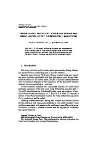
the deterministic problem are replaced here by two cones of forward dependence, which contain all the characteristics of the stochastic problem emanating from points 1 and 2 [Fig. 1(a)]. Suppose at this stage that we use the forward differencing for eqns (7) and (8). In that case the formulas for ?I,~and .rh3become

(9)

while those for pN and CJI,~ are



b)

Fig.

I. (a) Scatter in the characteristics finding the local average

emanating from points I and 2. (b) Windows involved random field k, at I, 2 and N from the microstructure.

in

Boundary value problems of random rigid-perfectly plastic media

PN

=PI

-@N+h)(PN-(PI)+

1123

-$a B

qN=

P,--P*+U7l(k,+kn)+P2(k*+kN)+~dS._-~dSg

n

1

(k,+kz+2kN)-,,

(10)

where ds, = [(x,,Yx,)2+(yN--Y,)2]“2

ds, = [(XN-x2)2+(yN--y2)2]“2

(11)

and the derivatives of k with respect to s, and s, are treated in the finite difference sense. The system (8) may also be solved via backward differencing. In the following, two other schemes are also considered, one recommended by Hill (1950), YN-_h

=

@N--XI)

tan

[(%

+~Nw+@i

YN-y2

=

(xN-x2)

tan

[((PZ

+(PN)/2-@19

(12)

and another, recommended by Szczepinski (1979), YN-_h

yN-Y2

=~(XN-Xl)[tan(% +@)+tan(qNf@)l = i(XN-X2)[tan ((P2-d4)+tan ((PN-n/4)l-

(13)

The exact method with the scheme (10) and (11) combined with either eqn (9), (12) or (13) forms the basis for determination of slip-line fields in the two types of boundary value problems studied below. In the remainder of this section we recall the considerations of Ostoja-Starzewski (1993) regarding the role of spacing of a finite difference slip-line net in relation to the micromechanics. To this end, consider the random microstructure to have the topology of a two-dimensional Voronoi-type mosaic of grains. Now, two characteristics a and /? of the continuum approximation of Fig. l(b) are indicated as passing through points 1 and 2, respectively, and crossing at the new point N. Three rectangular shaped windows B,(w), B,(o) and BN(w) centered at these three particular points represent three domains of the microstructure B(o), whose effective plasticities are described by k,, k2 and kN, respectively. Thus, we see that the finite differencing introduces a mesoscale between the microscale (grain scale) and the global macroscopic behavior. In the figure shown here, S z 18 in the a-direction and z 10 in the B-direction. In principle, due to the finite crystal size, these three quantities k,, k2, k3 cannot be taken as independent random variables, but should reflect the “local smearing out” in each window accounting for some correlation at their common boundaries. Effective plasticity of a given window is a function of plasticities of all the crystals belonging to that window, and hence may simply be modeled by a so-called moving average random field (Vanmarcke, 1983). Thus, at every location (x, y) the value kd is an average of plasticities of all the crystals in the window centered at (x,~). In other words, since all these crystals have random orientations, the average of their plasticities over a rectangular area with sides of length L, and L2, respectively, is a new random field kd with a covariance function C&(5,?) = {~~~(l-$)(I-!$)

Iand the shear stress is r,,., while the domain of influence lies in the first quadrant of the x,y-plane. The two following cases of boundary data were investigated in Ostoja-Starzewski (1992a) : a! = -1.5

z,,. = -0.6

6> = -1.5-s

7y,. =

(16)

-0.6.

Since, in view of eqn (4), the specification (17) gives rise to an inhomogeneous condition in the function p, we now consider

a! = - 1.5

7vy =

-0.6+

(17) boundary

X

Z

(18)

in order to investigate the effect of inhomogeneity in cp. In eqns (16)-(18) we take x = n. Ax for n = 0, 1, . . ,9 and Ax = 1.O. The sensitivity of these boundary value problems to the medium’s randomness is studied through a comparison of three cases : (i) deterministic case (medium &J-“zero

noise”

k = (k,)

(ii) random case-“very

small noise”-of

k:,

3

0;

0.5% about the mean

(19)

Boundary value problems of random rigid-perfectly plastic media k:, E[ (iii)

random case-“small

noise”-of

1125

-0.0025,0.0025];

(20)

5% about the mean

k:, E[-0.025,0.025].

(21)

In the above, (kd) = 1.0 and kiis a uniform random variate in a given interval. Comments on studies with Gaussian random variates are given in Section 5. Results of the boundary value problem (16) in the three cases (19), (20) and (21) are shown in Fig. 2(a), (b) and (c), respectively, while those of the boundary value problem (18) are shown in Fig. 3(a-c). Each of these figures was obtained from 100 simulation runs, using exactly the same sequence of pseudo-random numbers, according to the formulas (lo), (11) and (12), and employing backward differencing. Figure 2(a) and (c) here are practically the same as Fig. 2(a) and (c) in OstojaStarzewski (1992a), which used 1000 simulation runs. Thus, Fig. 2(b) here gives an indication of the effect of a very small randomness in the yield limit for the problem (16). On the other hand, Fig. 3(a-c) are analogous to Fig. 2(d) and (e) of Ostoja-Starzewski (1992a)

a)

b)

X

Fig. 2. The Cauchy problem with boundary data (16) for : (a) deterministic homogeneous mediumcase of zero noise; (b) random medium+ase of very small noise; (c) random medium-case of small noise. Cones of forward evolution are shown in (b) and (c)

M. Ostoja-Starzewski and H. Ilies

1126 Y4

a)

4

X

Fig. 3. The Cauchy problem with boundary data (18) for : (a) deterministic homogeneous mediumcase of zero noise ; (b) random medium-case of very small noise ; (c) random medium-case of small noise.

in that they display the amplifying effects of inhomogeneous boundary data on a small change of average slip-line net with respect to the homogeneous medium problem, as well as the scatter about this net. 4. THE CHARACTERISTIC

BOUNDARY

VALUE PROBLEM

The characteristic boundary value problem is defined as one in which the values of the function p and of the angle cp are given along the characteristics AB and AC belonging to two different families. Henceforth, y.(x) stands for AI3 and ya(x) stands for AC. In the present study the initial gradients of y&) and y&) are 45” and -45”, respectively, at the origin of an x, y-coordinate system. In order to study the effects of homogeneous versus inhomogeneous boundary data, this boundary value problem is studied here in four cases covering various combinations of y,(x) and yP(x) being either a straight line or a secondorder polynomial with positive or negative curvature. Thus, we have four boundary value problems :

Boundary value problems of random rigid-perfectly plastic media

1127

Problem no. 1 : yz=x

y$q= -x

(22)

ys=-x

(23)

Problem no. 2 :

y,=x+z

X2

Problem no. 3 : X2

y,=x+$j

X2

yg=x-_10

(24)

Problem no. 4 : y.=x-10

X2

ys=x-10.

X2

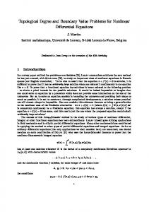
Inalltheabovewetakex=n.Axforn=0,1,...,9andAx=0.2. Numerical results of simulation of problem no. 1, in three cases of randomness (19), (20) and (21), are shown in Fig. 4(a-c), while those of problem no. 2 are shown in Fig. 4(d-f). Each of these figures was obtained from 100 simulation runs, using exactly the same sequence of random numbers, according to the formulas (9), (10) and (1 l), and employing backward differencing. One notes here a gradual increase in sensitivity of the slip-line nets to material randomness and to the inhomogeneity in the boundary data. This latter type of sensitivity is confirmed by Fig. 5, which gives solutions to problem no. 3 (a-c) and to problem no. 4 (d-f) in the three cases of randomness (19), (20) and (21); 100 simulation runs were also conducted here. 5. DISCUSSION

OF RESULTS

A study of all the boundary value problems leads to the following principal conclusions regarding the effect of noise k$ in the yield limit ks :

(0 there is practically no difference between the ensemble average net of slip-lines of the stochastic problem (i.e. for a random medium B) and the net of a corresponding deterministic problem (i.e. for a homogeneous medium Bdet) for very small noise ; however, this difference increases with the growing inhomogeneity in the boundary data ; (ii) the scatter about this average has a coefficient of variation which tends to quickly increase over that of k6 on the length scales of the boundary value problem ; it increases with growing inhomogeneity in the boundary data ; (iii) for noise growing above 5% [i.e. eqn (21)J there is an increasing change in the average, and very amplified scatter, in the random fields of stress as well as velocity ; as the type of change depends on a particular case, we do not demonstrate these here. Thus, we conclude that in the case of small noise one may replace the average solution ofa stochastic problem by the solution of a deterministic problem with keg = kdet = (kd) ; i.e. Bern= Bdet. Given the fact that the governing system (10) and (1 I), together with eqn (9) [or (12) or (13)], is a non-linear stochastic one, this is an interesting result. We correct here Ostoja-Starzewski (1992a, b), where it was concluded that there is always a change between the average and the deterministic solution ; this was due to a programming mistake in those references.

1128

M. Ostoja-Starzewski

b

x

and H. Ilies

FIG. 4

F

x

Fig. 4. The characteristic problem no. I with boundary data (22) for : (a) deterministic homogeneous medium--case of zero noise ; (b) random medium--case of very small noise ; (c) random mediumcase of small noise. The characteristic problem no. 2 with boundary data (23) for the same three cases is also shown : (d) zero noise ; (e) very small noise ; (f) small noise.

Moreover, we have found that there is practically (to within four significant figures) no difference in resulting slip-line nets between the explicit-formulas @)-and implicitformulas (12) or (13)-integration methods ; here, the explicit formulas were used first as

Boundary value problems of random rigid-perfectly plastic media

1129

a)

V

F X

FIG. S

+

X

Fig. 5. The characteristic problem no. 3 with boundary data (24) for : (a) deterministic homogeneous medium-case of zero noise ; (b) random medium-case of very small noise ; (c) random mediumcase of small noise. The characteristic problem no. 4 with boundary data (25) for the same three cases is also shown : (d) zero noise ; (e) very small noise ; (f) small noise.

a “predictor” and then, without any convergence problems, the implicit formulas were employed as a “corrector”. All results in Figs 3-5 were obtained under the assumption of independence of random variables ks at all the points of the finite difference nets. By introducing the correlation

M. Ostoja-Starzewski

1130

and H. Ilies

between neighboring windows, as discussed in the paragraph following eqn (13), the scatter in slip-lines tends to decrease, but only for 6 < 10, i.e. a very small mesoscale window, is this a significant effect. While all the figures presented in this paper were plotted using the exact method, we have determined that there was no difference between the average slip-line nets so obtained and the results of the mean field method ; to conserve space the latter are not given. We have also made a comparison of the uniform versus Gaussian randomness of k;. As an equivalence criterion between both kinds of probability distributions, we took the same standard deviation 0 for the case of very small noise (a = 14.43757 x lo-‘) and the case of small noise (0 = 144.3757 x 10e5). Since 12 uniform random variates were employed in the generation of each Gaussian one, the corresponding Gaussian distributions were always truncated at +6a, which, certainly, was more justifiable physically than the nontruncated case. With this set-up all our Gaussian-based simulations resulted in practically the same slip-line networks as the ones shown here.

6. LIMIT

ANALYSIS OF A CYLINDRICAL TUBE OF A RANDOM INHOMOGENEOUS PLASTIC MATERIAL UNDER INTERNAL PRESSURE

6.1. Tube of a homogeneous material In this section we give an application of our stochastic theory to the limit analysis of a cylindrical tube loaded by a uniform traction on the internal boundary ; this was first studied by Ostoja-Starzewski and Setyabudhy (1992). Solution to this classical problem in the case of a homogeneous material is based on the solution of a Cauchy problem for an axisymmetric stress field (o,, rr,,,,z,,) in an infinite plate, in plane strain, with a circular hole [see e.g. Kachanov (1971)]. For the so-called pressure boundary condition in polar coordinates

o’,. =

-p

< 0

Trv = 0

with or = -p < 0 and a, > 0 in the neighborhood

at

r = a,

(26)

of the hole, the yield condition being

ac -a,. = 2k.

(27)

The stress field is determined by the formula

a,. = -p+2k*ln

y ae = a,+2k. 0a ’

(28a,b)

The slip-line field is now given by a system of logarithmic spirals intersecting at an angle n/2 :

cp+ln

f 0

= c(, cp-ln

5a =P. 0

(29)

It follows from eqn (28a) that in the case of a tube of external radius 6, the condition u, = 0 at r = b gives the limit pressure

Boundary value problems of random rigid-perfectly plastic media

a)

b) Fig. 6. Slip-line patterns in a homogeneous material under : (a) pressure boundary condition (26), and (b) pressure and shear boundary condition (31).

p*=2k*ln

E .

(30)

0

The slip-line network corresponding to k = 1.5, p* = 3.0 and a = 1 is shown in Fig. 6(a), whereby eqn (30) is inverted to calculate b(p*) = a exp @*/2k) = 2.723 ; 30 nodes on the inner circumference are taken here. Henceforth we shall regard p* as given and the external radius b as a function of p*. In case of a pressure and shear boundary condition a, = -p

< 0

Zra

=q#O

at

r=a,

(31)

the slip-lines are no longer logarithmic spirals and the stress field is given by (Kachanov, 1971)

M. Ostoja-Starzewski and H. Ilies

1132

0,

=

-p&k

I

(Tg-(r,-

=

iJk’+ (4)‘.

Figure 6(b) shows the slip-line network corresponding to k = 1.5, p* = 3.0, y* = 1.3 and a = 1 ; these data result in the external radius b(p*, q*) = 3.028. 6.2. Tube qf a random inhomogeneous muterial In the case of a tube made of an inhomogeneous material, the net of slip-lines becomes distorted from the perfect patterns of Fig. 6(a) and (b). Formulas (28) and (32) no longer apply, and the system (10) and (1 l), and (9), (12) or (13), has to be used to determine the slip-lines as well as the stress field in any particular realization B6(m) of a spatially inhomogeneous medium of the family &. We recall here the final note of Section 3. However, the evolution of cr, along any outgoing slip-line is a certain random walk, in the body domain D, starting from -p* at r = a and stopping at 0 at r = b. Thus, the condition cr, = 0 plays the key role in the definition of an excursion set of a random field c,(r, cp) = {cr(o) ; o ESZ} [see e.g. Adler (1981)] A,(o,,D)

= {(r,cp)EDIo,(r,cp)

B O}.

(33)

This then leads to the definition of a so-called set of level crossings : d&(o,.,D)

= {(r,v)EDbr(r,cp)

= 0).

(34)

The set a&(~~, D) is a set of closed contours of the plastic zone, which in the case of a homogeneous material Bdetunder the pressure boundary condition would be a circle of radius b(p*) = 2.723. Thus, in any given inhomogeneous material the set of level crossings is a random set in plane, which, due to the spatial homogeneity of field ks, is a circular ring containing all the possibilities. Let b,,, and b,,, be a maximum and minimum distance for a given realization, respectively, from the origin to the contour. Since b,,, determines the minimal amount of material needed for a tube to withstand the internal pressure p*, the natural questions to ask are : Ql : “Is b,,,(p*) smaller, equal to or larger than b(p*) of the homogeneous medium problem?” Q2 : “What is the probability distribution of b,,, and b,,,?” 43 : “What is the effect of shear traction in boundary condition (31) versus (26)?” Two particular cases of noise were investigated : k:, E [ -0.0094,0.0094]

(35)

kl, E [ -0.025,0.025].

(36)

and

In Fig. 7(a) we plot patterns of slip-lines under condition (26) corresponding to 400 realizations B6(a) of a random medium with (kd) = 1.5 and k’, sampled according to

Boundary value problems of random rigid-perfectly plastic media

1133

b)

Fig. 7. Slip-line patterns in a randomly inhomogeneous material, with & following (36), under : (a) boundary condition (26) and (b) boundary condition (31). In each case, 400 realizations of B(o) are used.

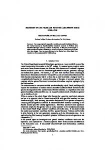
condition (36). The set of level crossings is shown as a ring containing all 400 piecewiseconstant non-circular closed curves. Next, in Fig. 7(b) we plot slip-line patterns for the same type of medium under condition (31), also for 400 realizations. Finally, in Fig. 8(a) and (b) we plot the probability distributions of b,,, and b,, for the cases, respectively, of the pressure boundary condition (26), and of the pressure and traction boundary condition (3 1). In order to demonstrate the sensitivity to random noise in the yield function, in each of these two figures we show data corresponding to conditions (35) and (36). It follows now that the answer to the first question is “always larger”, whereby b,,, increases as the noise level in ki increases. Thus, the principal conclusion is that the presence of material inhomogeneities requires a thicker tube than that predicted by the homogeneous medium theory. Let us note here that the higher the pressure p, the greater is the external SAS 33-8-E

M. Ostoja-Starzewski and Hf. Ilies

1134 (a) 0.9 -

0.6 0.7 0.6 0.5 0.4 0.3 0.2 -

b(p')= 2.723

(b)

0.8 0.7 0.60.5 0.4 0.30.2 -

b(p’, q’) = 3.028

Fig. 8. Probability distributions P(b,) (35), P(b,,,) (36), P(b,,,) (35) and P(b,,,) (36) for the cases: (a) of pressure boundary condition (26) and (b) pressure and shear boundary condition (31) ; /ii is sampled according to conditions (35) and (36). In each case 400 realizations of B(w) are used. The deterministic cases be*) = 2.723 and b(p*, q*) = 3.028 are also shown.

radius 6, and hence the greater is the spread of the forward evolution cones, implying an increase in the scatter of b,,, and b,i,. Interestingly, both random variables b,,, and bmin are symmetrically distributed about the deterministic radius b(p*) of the homogeneous

Boundary value problems of random rigid-perfectly plastic media

medium problem ; this answers Q2. The same qualitative conclusions carry of the pressure and shear boundary condition, but one must note here that shear traction has a strongly amplifying effect on the scatter of dependent and most notably the spread of slip-lines [compare Fig. 7(a) and (b)] ; this

1135

over to the case the addition of field quantities, addresses 43.

7. CLOSURE

We note first that random distortions of slip-line patterns from those predicted by deterministic medium theory are observed in experiments [see photographs in Kachanov (1971) and Mellor and Johnson (1985); note also Alpa and Gambarotta (1990)]. Our approach allows an assessment of such random noise via the determination of the statistics of slip-lines and stress fields. As mentioned in the Introduction, plasticity of random inhomogeneous media has recently been studied by Nordgren (1992) with a focus on stochastic theorems on limit load coefficients and an application to the loading of a wedge. Solution of this latter problem has been based on finding the mean of the minimum energy dissipation on the multiple branches of possible zig-zag velocity paths along the rigidplastic boundary. This methodology differs from ours : we propose solving a given stochastic boundary value problem directly by calculating a large number (100, say) of responses in a Monte Carlo sense. Unless the mesh resolution is more than about 50 points, this is done in a matter of (at the most) a couple of minutes on a workstation or a personal computer and yields practically the whole range of possible behaviors, i.e. the probability distributions of slip-line fields and stress fields. This is in contrast to a study by Nordgren (1992), which reports a need for extensive computational tasks. We would also like to point out that our method of a mesoscale random continuum model applies to the determination of the velocity fields, and can be extended to hardening behavior and anisotropic yield conditions. Indeed, as pointed out in Section 2.3, anisotropic yield conditions of random character are expected from a micromechanical derivation ; research on that subject is in progress. Finally, it is of interest to mention that the present study is related to another topic: transient stress waves in randomly inhomogeneous media (Ostoja-Starzewski, 1991). The common feature is the fact that, mathematically, both these problems are stochastic quasilinear hyperbolic systems. They both display Markov properties and share the concepts of forward evolution cones in place of unique characteristics of deterministic homogeneous media problems. However, the major difference between them lies in that the spacing of characteristics in a plasticity problem corresponds directly to a mesoscale, while no such mesoscale concept appears in the wavefront studies.

Acknowledgements-Support by the National Science Foundation under grant no. MSS 9202772 and during a visit at the Institute for Mechanics and Materials at the University of California, San Diego is gratefully acknowledged. The authors benefited from discussions with Professor S. Zargaryan of the UCSD.

REFERENCES Adler, R. J. (1981). The Geometry of Random Fields. John Wiley, New York. Alpa, G. and Gambarotta, L. (1990). Probabilistic failure criterion for cohesionless frictional materials. J. Mech. Phys. Solids 38,491-503.

Hill, R. (1950). The Mathematical Theory of Plasticify. Oxford University Press, London. Kachanov, L. M. (1971). Foundations of the Theory of Plasticity. North-Holland, Amsterdam. Mellor, W. and Johnson, P. B. (1985). Engineering Plasticity. Ellis Horwood/John Wiley, Chichester/New York. Nordgren, R. P. (1992). Limit analysis of a stochastically inhomogeneous plastic medium with application to plane contact problems. ASME J. Appl. Mech. 59,477-484. Olszak, W., Rychlewski, J. and Urbanowski, W. (1962). Plasticity under inhomogeneous conditions. Ado. Appl. Mech. 7, 132-214.

Ostoja-Starzewski, M. (1991). Transient waves in a class of random heterogeneous media. Appl. Mech. Rev. (special issue: Mechanics Pan-America 1991) 44 (10, Part 2), Sl99-S209. Ostoja-Starzewski, M. (1992a). Plastic flow of random media : micromechanics, Markov property and slip-lines. Appt. Mech. Rev. (special issue : Material Instabilities) 45 (3, Part 2), S75-S81.

1136

M. Ostoja-Starzewski and H. Ilies

Ostoja-Starzewski, M. (1992b). Boundary value problems in plastic flow of random media, ASME Summer Mechanics and Materials Conference. In Plastic Flow and Creep (Edited by H. Zbib), Vol. AMD135-MD31, pp. 149-l 58. ASME, Philadelphia. Ostoja-Starzewski, M. (1993). Micromechanics as a basis of stochastic finite elements and differences-an overview. Appl. Mech. Rev. (special issue: Mechanics Pan-America 1993) 46 (11, Part 2), S136-S147. Ostoja-Starzewski, M. (1994). Micromechanics as a basis of continuum random fields. Appl. Mech. Rev. (special issue : Micromechanics of Random Media) 47 (1, Part 2), S221-S230. Ostoja-Starzewski, M. and Setyabudhy, R. (1992). Limit analysis of a cylindrical tube of a random inhomogeneous plastic material under internal pressure, ASME Winter Annual Meeting. Recent Advances in Sfructural Mechanics (Edited by Y. W. Kwon and H. H. Chung), Vol. PVP248-NEIO, pp. 87-92. ASME, Philadelphia. Szczepinski, W. (1979). Introduction to the Mechanics of Plastic Forming of Metals. Sijthoff & Noordhoff Int. Publ./PWN, Alphen an der Rijn/Warsaw. Vanmarcke, E. H. (1983). Random Fields: Analysis and Synthesis. MIT Press, Cambridge, MA.