THE CENTERED DISCRETE FRACTIONAL FOURIER TRANSFORM AND LINEAR CHIRP SIGNALS Juan G. Vargas-Rubio† and Balu Santhanam University of New Mexico, Albuquerque, NM 87131 Tel: 505 277-1611, Fax: 505 277-1439 Email: jvargas,
[email protected]
1. INTRODUCTION The basis functions of the kernel of the continuous fractional Fourier transform (FRFT) are chirp signals, where a closed-form expression relating the angle of the transform and the chirp rate of the signal whose transform is a delta function exists. For most of the discrete versions of the fractional transform [1, 2, 3], however, this is not the case because these transforms are derived from the eigenvalue– eigenvector decomposition of some version of the discrete Fourier transform (DFT), and there is no closed form for the elements of the resulting matrices. A discrete FRFT that is based on a centered version of the DFT (CDFRFT) was considered in [5, 6] and its properties were studied in [6]. Specifically it was shown that the basis functions of the CDFRFT contained both amplitude and frequency modulation and that the instantaneous frequency (IF) of the basis functions are sigmoidal. However, for the discrete case, there † This author is also with: Universidad Aut´ onoma Metropolitana Az´ capotzalco, Departamento de Electr´onica, M´exico, DF 02200, MEXICO, Tel: +52 55 5318-9034
0-7803-8434-2/04/$20.00©2004 IEEE
2
CDFRFT of x[n]=ej0.005*n for alpha=102° 8 7 6
MAGNITUDE
ABSTRACT The basis functions for the fractional Fourier transform are chirp signals where a precise relationship between the fractional parameter and the chirp angle can be established. The recently introduced centered discrete fractional Fourier transform, based on the Gr¨unbaum commuting matrix, has basis functions that have a sigmoidal instantaneous frequency and produces a transform that is approximately an impulse for discrete chirps. However, no such precise relation between the fractional parameter and the chirp rate of the basis functions exists in the discrete case. In this paper, we study the relationship between the chirp rate and the fractional parameter in the discrete case and specifically look at two approximate expressions that relate the chirp rate and the angle for which one obtains a impulse– like transform. We study the efficacy of these estimates by applying them to the analysis of monocomponent and two component chirp signals.
5 4 3 2 1 0 0
20
40
60 80 FREQUENCY
100
120
140
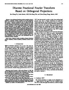
Fig. 1. Concentrating a chirp: CDFRFT with α = 102◦ compared with the CDFT of the signal (dotted lines).
exists no exact relation between the chirp rate of a signal and the angle of the transform. In this paper, we first demonstrate that the CDFRFT has the capability of concentrating the energy of a linear chirp in a few transform coefficients for a specific angle. We then present two approximate empirical expressions relating the chirp rate to the angle that produces an impulse-like transform and evaluate the efficacy of these expressions by applying them to the analysis of monocomponent and two component chirp signals. 2. THE CENTERED DFRFT We define the CDFRFT for parameter α as Aa = VT Λ2α/π VT H ,
(1)
where VT is the matrix of orthogonal eigenvectors obtained from the Gr¨unbaum [5] commuting matrix T. The eigenvectors are in descending order with respect to its corresponding eigenvalue in T, that is, the first column of VT corresponds to the eigenvector with larger eigenvalue. Λ2α/π is diagonal with elements λk = e−jkα , 0 ≤ k ≤ N − 1. With
163
RELATION BETWEEN CHIRP RATE AND ALPHA FOR N=128
this substitution the definition becomes: Aα =
N −1 X
0.5 0.4
e−jαk vk vkH .
0.3
(2)
0.2
Using the definition of the CDFRFT, we now develop a fast algorithm for computing the multiple angle version of the CDFRFT. The elements of the CDFRFT matrix can be expressed as N −1 X p=0
vkp vnp e−jpα ,
0.1 0 −0.1 −0.2 −0.3 −0.4 −0.5 0
0.5
1
1.5
2
2.5
3
ALPHA
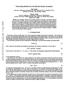
Fig. 3. Relation between chirp rate and angle for N = 128. The solid line corresponds to the approximation in Eq. (10)
where vkp is the k-th element of p-th eigenvector . Multiplying Aα by the signal x[n] we obtain the transform: Xα [k] =
N −1 X
x[n]
n=0
N −1 X
vkp vnp e−jpα ,
(4)
p=0
and after rearranging the two sums we obtain: Xα [k] =
N −1 X
vkp
p=0
N −1 X
x[n]vnp e−jpα .
(5)
n=0
If we use a discrete set of angles given by α = αr =
2πr , r = 0, 1, . . . , N − 1, N
(6)
we obtain Xr [k] =
N −1 X p=0
vkp
N −1 X
2π
x[n]vnp e−j N pr .
(7)
n=0
Defining zk [p] as zk [p] = vkp
N −1 X
x[n]vnp ,
(8)
n=0
we observe that the transform can be expressed as the DFT of zk [p], that is
3. THE MULTI–ANGLE CDFRFT
{Aα }kn =
CHIRP RATE
k=0
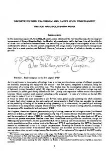
This definition assigns the eigenvectors via the ordering of the eigenvalues of T and assigns the eigenvector with m sign changes to the eigenvalue λm = e−jmα and this is the same correspondence between the continuous FRFT and Hermite–Gauss functions. It is specifically instructive to observe that the basis functions of the CDFRFT, i.e., the rows of the CDFRFT matrix for any given α are not complex linear chirps with constant amplitude and chirp rate. This fractional transform becomes identity for α = 0◦ , where the basis functions are shifted delta functions. For α = 90◦ it becomes the CDFT, whose basis functions are complex exponentials of constant frequency and amplitude [1]. Fig. 2(a) describes this transformation for a particular basis vector for angles from zero to 180◦ . It has also been shown in [6] that the instantaneous frequency of the basis functions for intermediate angles is sigmoidal rather than linear as described in Fig. 2(b) for α = 5◦ . The frequency goes from −π to π in all rows and the transition is very sharp. As the angle increases, the changes in frequency are much smaller as it shown in Fig. 2(c) for α = 85◦ where the slope of the curves is very small and the frequency of each row is almost constant. To understand the ability of the CDFRFT to concentrate a chirp signal in a few transform coefficients, let us look 2 at the complex signal x[n] = ej0.005n , with 0 ≤ n ≤ 127, that has a constant chirp rate. Trial and error determines that α = 102◦ produces a good concentration in the transform. Fig. 1 shows the result compared with the dotted lines that are the CDFT (α = 90◦ ) of the same signal. We observe that the transform with α = 102◦ produces a sharp peak whose smallest and largest components occur at the frequencies of 0.6136 and 0.6627 with average frequency 0.645. From the results of the example, we can observe that: (a) we can concentrate a linear chirp in a few transform coefficients with the CDFRFT, (b) the concentration occurs close to the average frequency.
Computed π tan(alpha−π/2)/128
(3)
Xk [r] =
N −1 X
zk [p]WNpr , 0 ≤ r, k ≤ N − 1.
(9)
p=0
Expressing the transform as a DFT allows us to use the regular FFT algorithm for computing the CDFRFT. The resulting transform Xk [r] containing the CDFRFT for these discrete angles is called the multi–angle DFRFT (MADFRFT).
164
N=128, angle=5.00°
ROW 75, N=128
N=128, angle=85.00°
3
2
frequency
1
frequency
alpha 180° 2 162° 1 144° 126° 0 108° 90° −1 72° −2 54° 36° −3 18° 0° (a)
3
0 −1 −2 −3
20
40
60 index
80
100
120
20
(b)
40
60 index
80
100
120
(c)
Fig. 2. (a) Transformation of one of the basis vectors (row) of the CDFRFT as the fractional angle α goes from 0◦ to 180◦ . (b) IF estimates for the rows of the CDFRFT matrix with N = 128 and α = 5◦ and (c) IF estimates for α = 85◦ . 4. RELATING CHIRP RATE & ANGLE The approach used here is to find the chirp rate of the signal that results in the largest peak in the magnitude of the MADFRFT for a the discrete set of angles defined before. We first look at complex chirps with zero average frequency of the form N −1 2 2 )
x[n] = ejcr (n−
, 0 ≤ n ≤ N − 1,
where cr is the chirp rate. After performing the computation for different sizes transform sizes, the results show that the relation between the chirp rate cr and angle α can be described approximately by the relation cr = π
tan(α − π/2) . N
(10)
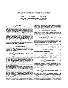
This relation is not exact and has an error slightly larger than 10% for some angles. A plot of the results for N = 128 is given in Fig. 3. The other aspect of this approximation that we wish to determine is how good the concentration of the chirp function for the values obtained before is. For this purpose we computed the number of coefficients of the transformed signal that captured 50% of the total energy. The result of this computation reveals that we only get good concentration of the chirp signal in the interval of angles from 45◦ to 135◦ , and in this range, 50% of the energy is concentrated in at most two coefficients. Outside the interval the number of coefficients grows rapidly, as it can be seen in Fig. 4(a). Let us now consider the case of chirp signals having an average frequency different than zero, i.e., 2
x[n] = ej(cr (n−(N −1)/2)
+ω0 (n−(N −1)/2))
, 0 ≤ n ≤ N −1.
where ω0 is the average frequency. The other point of interest is where the maximum concentration occurs and is a
measure of how well the CDFRFT can localize the average frequency of this chirp signal. In addition to the computation of the chirp rate and the number of coefficients needed for capturing 50% of the energy, we also compute the coefficient at which the maximum value occurs. The results show little difference in the relation of the chirp rate with the angle α compared with the case of zero average frequency. The number of coefficients that concentrate 50% of the energy of the signal is also similar to the zero average frequency case, but as the average frequency increases, the interval for which we concentrate the signal in two coefficients decreases slightly. Fig. 4(b) shows the case for ω0 = 1.57. The error in the localization of the average frequency, measured as the difference between the coefficient of the average frequency and the coefficient at which the peak occurs, shows that as the average frequency increases, the error also increases. Fig. 4(c) shows this difference for positive frequencies. The larger deviations correspond to larger frequencies. This result is also affected by aliasing and consequently we ignore combination of large chirp rate and large average frequency. From the results in previous sections, we see that for alpha between 45◦ to 135◦ we obtain better concentration of signal energy when analyzing linear chirps. For this interval, we have found empirically that the relation between the angle of the transform and the chirp rate can be approximated better if we add a linear term to Eq.(10) and the corresponding error is reduced to less than 2% : cr = 2
(α − π/2) tan(α − π/2) + 1.41 . N N
(11)
This relation is useful for determining the chirp rate from the angle at which we have more concentration, particularly when we the MA-CDFRFT algorithm described before is used.
165
NUMBER OF COEFFICIENTS WITH AT LEAST 50% OF THE ENERGY forω0=1.57 and N=128
NUMBER OF COEFFICIENTS WITH AT LEAST 50% OF THE ENERGY, N=128 16
DIFFERENCE BETWEEN THE ACTUAL COEFFICIENT AND THE COEFFICIENT OF THE AVERAGE FREQUENCY
14
14 14 12
12
10
8
6
NUMBER OF COEFFICIENTS
10 NUMBER OF COEFFICIENTS
NUMBER OF COEFFICIENTS
12
8
6
10
8
6
4
4
4
2 2
2
0
0
0.5
1
1.5 ALPHA
2
2.5
3
0
(a)
0
0
0.5
1
1.5
2
2.5
ALPHA
3
3.5
−2
(b)
0.8
1
1.2
1.4
1.6 ALPHA
1.8
2
2.2
(c)
Fig. 4. (a) Number of coefficients capturing 50% of chirp signal energy as a function of α with w0 = 0, (b) with w0 = 1.57, (c) number of coefficients of error in the localization of the average frequency with respect to α. 5. EXAMPLES: CHIRP RATE ESTIMATION Our goal in this section, is to study the utility of the two approximate expressions relating the chirp rate to the transform angle. The first example pertains to the application of the MA-DFRFT to a single linear chirp signal: x[n] = ej(0.005(n−
127 2 2 ) )
, 0 ≤ n ≤ 127
Fig. 5(a) shows the complex chirp signal, Fig. 5(b) describes the magnitude of the MA-DFRFT of this signal. Specifically we observe that we actually have two maxima because the CDFRFT at α + π is reversed version of the CDFRFT at α. The location of the maximum is at r = 36 which corre36 sponds to an angle α = 2π 128 = 1.7671. Upon application of Eq. (10) the corresponding chirp rate estimate is 0.0049, while application of Eq. (11) yields a chirp rate of 0.0053. Fig. 5(c) is the slice of the MA-DFRFT at this particular angle, where the magnitude of the MA-DFRFT is a maximum. Adding another chirp component with zero average frequency at a different chirp rate yields a two-component chirp signal. The MA-DFRFT and the approximate relations are applied to estimate the two chirp rates associated with the two-component chirp signal. The second chirp component has a negative chirp rate of 0.007. For this case the maxima occur at r = 36 and r = 27 and the corresponding chirp rates from application of Eq. (10) are 0.0049 and 0.0062. The corresponding chirp rates obtained via Eq. (11) are 0.0053 and -0.0066. The chirp signal, its MA-DFRFT and its slice at the angle where the magnitude of the MADFRFT is a maximum are shown in Fig. (5). In both cases, we can see that the MA-DFRFT is able to concentrate chirp signals into a few coefficients and that Eq. (10) and Eq. (11) can be used to estimate the chirp rate(s) of the signal.
6. CONCLUSION In this paper, we have studied the capability of the centered DFRFT obtained from the Gr¨unbaum commuting matrix to concentrate a chirp signal in a few transform coefficients. We presented an FFT based algorithm for computing the multi-angle version of the CDFRFT. We then furnished two empirical relations that related the chirp rate and the angle that produced a impulse-like transform. We evaluated the efficacy of these expressions by applying these relations to the analysis of single and two component chirps signals and demonstrated that the CDFRFT and its multi-angle version are powerful time-frequency tools for the analysis of both monocomponent and multicomponent chirp signals. 7. REFERENCES [1] B. Santhanam and J. H. McClellan, ”The Discrete Rotational Fourier Transform,” IEEE Trans. Sig. Process., Vol. 44, No. 4, pp. 994-998, 1996. [2] S. Pei, M. Yeh, C. Tseng, ”Discrete Fractional Fourier Transform Based on Orthogonal Projections,” IEEE Trans. Sig. Process., Vol. 47, No. 5, pp. 1335-1348, May 1999. [3] C. Candan, M. A. Kutay, H. M. Ozatkas, ”The Discrete Fractional Fourier Transform,” IEEE Trans. Sig. Process. , Vol. 48, No. 5, pp. 1329-1337, 2000. [4] D. H. Mugler and S. Clary, ”Discrete Hermite Functions and The Fractional Fourier Transform,” in Proc. Int. Conf. Sampl. Theo. and Appl. Orlando Fl, pp. 303-308, 2001 [5] S. Clary and D. H. Mugler, ”Shifted Fourier Matrices and Their Tridiagonal Commutors,” SIAM Jour. Matr. Anal. & Appl., Vol. 24, No. 3, pp. 809-821, 2003. [6] B. Santhanam and J. G. Vargas-Rubio, ”On the Gr¨unbaum Commutor Based Discrete Fractional Fourier Transform,” Proc. of ICASSP04, Vo. II, pp. 641-644, Montreal, 2004. [7] J. G. Vargas-Rubio and B. Santhanam, ”Fast and Efficient Computation of a Class of Discrete Fractional Fourier Transforms” Submitted IEEE Sig. Process. Lett., March 2004.
166
MA−DFRFT OF THE SIGNAL
REAL PART
SLICE OF THE MA−DFRFT AT r = 36 0.7
1 120
0.5 0.6 100
0
0.5
0
20
40
60
80
100
120
140
IMAGINARY PART 1
80 MAGNITUDE
−1
INDEX r (ANGLE)
−0.5
60
0.4
0.3
40
0.5
0.2
0
20
0.1
−0.5 0
−1
0
20
40
60
80
100
120
140
0
(a)
20
40
60 80 INDEX k (FREQUENCY)
100
120
0
(b)
0
20
40
60 80 INDEX k (FREQUENCY)
100
120
140
(c)
Fig. 5. Monocomponent chirp: (a) chirp signal with a chirp rate, (b) magnitude of the corresponding MA-DFRFT, and (c) slices of the MA-DFRFT at r = 36.
MA−DFRFT OF THE SIGNAL
REAL PART
SLICE OF THE MA−DFRFT AT r = 36 0.8
2 120
0.6 MAGNITUDE
1
100
0
0
20
40
60
80
100
120
INDEX r (ANGLE)
−2
0.4
0.2
−1
140
IMAGINARY PART 2
80 0
0
20
40
60
60 80 INDEX k (FREQUENCY)
100
120
140
100
120
140
SLICE OF THE MA−DFRFT AT r = 27 0.7 0.6
0
MAGNITUDE
40
1
20
−1
0.4 0.3 0.2 0.1
0
−2
0.5
0
20
40
60
80
100
120
140
(a)
0
20
40
60 80 INDEX k (FREQUENCY)
100
120
0
(b)
0
20
40
60 80 INDEX k (FREQUENCY)
(c)
Fig. 6. Two component chirp: (a) composite signal, (b) magnitude of the corresponding MA-DFRFT, and (c) slices of the MA-DFRFT at r = 36 and r = 27.
167