DISCRETE AND CONTINUOUS DYNAMICAL SYSTEMS Supplement 2013
Website: www.aimSciences.org pp. 393–406
THE CHARACTERIZATION OF MAXIMAL INVARIANT SETS OF NON-LINEAR DISCRETE-TIME CONTROL DYNAMICAL SYSTEMS
Byungik Kahng Department of Mathematics and Information Sciences University of North Texas at Dallas Dallas, TX 75241, USA
Miguel Mendes Departamento de Engenharia Civil Faculdade de Engenharia da Universidade do Porto Rua Dr. Roberto Frias 4200 - 465 Porto, Portugal
Abstract. The main topic of this paper is the controllability/reachability problems of the maximal invariant sets of non-linear discrete-time multiplevalued iterative dynamical systems. We prove that the controllability/reachability problems of the maximal full-invariant sets of classical control dynamical systems are equivalent to those of the maximal quasi-invariant sets of disturbed control dynamical systems, when modeled by the iterative dynamics of multiple-valued self-maps. Also, we prove that the afore-mentioned maximal full-invariant sets and maximal quasi-invariant sets are countably infinite step controllable under some appropriate conditions. We take an abstract set theoretical approach, so that our main theorems remain valid regardless of the topological structure of the space or the analytical structure of the dynamics.
1. Introduction. The usefulness of maximal/minimal invariance in non-linear control and automation theory is well known and well established. See, for instance, [7] for a through survey on the history of this topic, and [2, 5, 12, 20, 21, 22, 27, 30, 31, 32, 33, 34, 35, 36] for more modern trend. The topic of the authors’ particular interest is the controllability/reachability problems of the locally maximal invariant sets. For more detail, see [14, 15, 16, 18], and also, [13, 19]. The purpose of this article is to provide the mathematical background of the authors’ earlier contributions they just listed. The main focus of attention being the application to engineering, [14, 15, 16, 18] greatly abridged or altogether skipped the proofs of some important lemmas, upon which their main theorems and computational algorithms were based. The present paper will fill in this gap. The study of the maximal/minimal invariant sets has a rich history that dates back at least to the turn of the 20th century. See, for example, [1] for a through review on this topic including its history. The focus of our attention is the controllability/reachability problems of the locally maximal invariant sets. This topic is attracting plenty of attention these days from both pure and applied mathematics. 2010 Mathematics Subject Classification. Primary: 93C05, 93C25, 93C55; Secondary: 37E99. Key words and phrases. Maximal invariance, controllability, orbit-chain.
393
394
BYUNGIK KAHNG AND MIGUEL MENDES
See, for instance, [8, 23, 24, 25], for some examples of recent use of the locally maximal invariance in pure mathematics, particularly in C 1 -stability of diffeomorphic dynamical systems and their hyperbolicity problems. Also in applied mathematics, this classical topic is receiving a renewed attention these days, as evidenced by a substantial number of recent contributions on this topic, some of which were listed in the first paragraph. One reason behind such revival is the resurgence of nonlinear control dynamical systems with chaotic disturbance. For the most part, this is because “the improvements in computational capabilities have made it possible to implement the algorithms for systems of practical interest,” as [20] explains. The computational algorithm is, of course, an approximation through a finite number of steps. Therefore, it is necessary to prove when/whether such an approximation is indeed meaningful. Also, there is another issue that is more important for the purpose of this paper. The disturbed control dynamical systems were considered in classical control and automation theory too, say, [6], but not to the extent that the disturbance changes the qualitative properties or to create the bifurcation of the dynamics, as we do here. This direction of research was partly inspired by the study of the dynamical systems that are disturbed by singularities such as kicks and pulses, which is a rapidly growing topic in non-linear physics and mathematics. See, for instance, [3, 4, 9, 10, 11, 17, 26, 28, 29]. This is nothing more than an incomplete list among a large number of recent contributions on this topic, selected specifically for their direct connection to the invariant set theory of control dynamical systems. The authors believe that the inclusion of the singularities is a reasonable assumption to explore as a new frontier of nonlinear control dynamical systems and automation theory, because nonlinear and chaotic phenomena caused by singular disturbances such as kicks and pulses are abundant in nature and so are the demands to control them automatically. Furthermore, the singularities of the control dynamical systems do not always come from the singularities of the disturbances. Even in such a common control system like the automatic transmission system of passenger cars, it is not unusual that the sudden jolt kicks in as one controller replaces another, particularly during the up-hill driving. Whether the singularities of the control dynamical systems come from the disturbances, from the multiple controllers, or from still difference sources, the authors believe that it is worth studying them in any case. From this point on, therefore, we will not assume the continuity of the dynamics and/or the feedback-controls. One of the main difficulties regarding the control dynamical systems with singularities is that many of the well-known results of the classical control and automation theory had to be either discarded or adjusted. In this paper, we pay particular attention to the controllability/reachability problems of the maximal invariant sets (Definition 2.1 and Definition 2.2). In classical control theory, all maximal invariant sets are always countably-infinite step controllable, so the finite-step approximation algorithms can be used (Remark 2.4). If we do away with the continuity condition, however, the equality (2.10) no longer holds in general, and thus the approximation algorithm (2.11) becomes meaningless. The first main result of this paper is to reestablish and generalize such classical results, under some suitable conditions (Main Theorem 1). We use the backward orbit-chain method as the main tool (Definition 3.1, Theorem 3.2 and Theorem 3.3). Our second main result, Main Theorem 2 begins with a duality. We use, this time, the forward orbit-chain method as the main tool (Definition 4.1 and Theorem
THE CHARACTERIZATION OF MAXIMAL INVARIANT SETS
395
4.2). Along the way, we show that the solutions of the controllability/reachability problems of the maximal full-invariant sets of classical control dynamical systems are equivalent to those of the maximal quasi-invariant sets of disturbed control dynamical systems, up to the directions of the iterations. Since the latter systems may contain singularities, randomness, uncertainty, and so on, we argue that the former systems must be treated the same way. This way, we can establish the equivalence (or, the duality) and use it to further investigate the modern disturbed control dynamical systems. The rest of this paper is structured as follows. In Section 2, we discuss the control dynamics models of our interest, make necessary definitions, and then, state the main theorems of this paper. The next two sections concern the proofs of the main theorems. Section 3 deals with Main Theorem 1. Its conclusion is not too different from well known classical results, but we establish it without the continuity condition. Section 4 proves Main Theorem 2, through which we study modern models of disturbed control dynamical systems with uncertainty. Section 5 briefly summarizes the main results and the directions of future research. The final section, Section 6, is an appendix that complements Section 3 with an example that supports the key requirement of Main Theorem 1. 2. Definitions and main theorems. It is easy to see that the classical undisturbed non-linear time-invariant discrete-time control dynamical system given by a pair of maps f : X × U → X and g : X → U , where ( f : (xk , uk ) 7→ xk+1 , (2.1) g : xk 7→ uk , can be reduced to the iterative dynamical system, or the closed loop system, of one self-map, ψ : X → X, ψ(x) = f (x, g(x)). It is not easy, however, to do the same in the presence of disturbance. Introducing the disturbance variables, one can model a disturbed control dynamical system (DCDS) by the maps f : X × U × W → X and g : X → U , where ( f : (xk , uk , wk ) 7→ xk+1 , (2.2) g : xk 7→ uk . See, for instance, [20, 21, 32, 33] for more detail on this approach. However, the model (2.2) cannot be reduced to an iterative dynamical system (closed loop system), unless we know in advance which disturbance will take place at which time. One way to solve this difficulty is the use of the iterative dynamical system of a multiple-valued self-map, to model a DCDS, as proposed in [2]. A multiple-valued self-map (or a set-valued self map) φ on the set (or phase space) X is a map on its power set P(X) with the property that [ φ(S) = {φ(x) : x ∈ S}, ∀S ⊆ X. (2.3) Here, we used the traditional abbreviation, φ(x) for φ({x}) and φ−1 (x) for φ−1 ({x}), which we will continue throughout the paper. Under these considerations, one can express and generalize the model (2.2) as follows. ψ(S) = {f (x, g(x), w) : x ∈ S, w ∈ W }.
(2.4)
It is possible to prove that the multiple-valued iterative dynamical system (MVIDS) given by (2.4) is well-defined according to the equality (2.3), and generalizes the
396
BYUNGIK KAHNG AND MIGUEL MENDES
previous model (2.2) [16]. Also, see [19] for more detail on how MVIDS can be used to close up the open loops, and why every discrete-time DCDS can be modeled by MVIDS. Finally, see [2] and [33] for a similar utilization of a MVIDS to model a DCDS. Although our focus of attention is the maximal invariance and that of [2, 33] is the minimal invariance, the use of the MVIDS turns out to be a powerful tool for both approaches. Because it is possible to reduce general discrete-time DCDS to a closed-loopsystem through MVIDS, we now confine ourselves to the closed loop systems only. The distinction between the classical and the modern control dynamics models will be, from this point on, whether the iterative dynamics of ψ is single-valued, or multiple-valued (set-valued). Definition 2.1. Let X be a nonempty set and ψ : X → X be a single-valued self-map. We say S ⊆ X is full-invariant under ψ if ψ(S) = S, and it is quasiinvariant under ψ if ψ(S) ⊆ S. Also, given nonempty subset Y of X, we define the locally maximal full-invariant set M(Y ) and the locally maximal quasiinvariant set M+ (Y ) as, [ M(Y ) = {S ⊆ Y : ψ(S) = S}, (2.5) and M+ (Y ) =
[ {S ⊆ Y : ψ(S) ⊆ S},
(2.6)
respectively. Definition 2.2. Let X be a nonempty set and ψ : P(X) → P(X) be a multiplevalued self-map. That is, [ ψ(S) = {ψ(x) : x ∈ S} (2.7) for all S ⊆ X. We say S ⊆ X is strongly quasi-invariant under ψ if ψ(S) ⊆ S, and it is weakly quasi-invariant under ψ if ψ(x)∩S 6= ∅ for all x ∈ S. Also, given nonempty subset Y of X, we define the locally maximal strong quasi-invariant + set M+ s (Y ) and locally maximal weak quasi-invariant set Mw (Y ) as, [ M+ {S ⊆ Y : ψ(S) ⊆ S}, (2.8) s (Y ) = and M+ w (Y ) =
[
{S ⊆ Y : ψ(x) ∩ S 6= ∅, ∀x ∈ S},
(2.9)
respectively When there is no danger of confusion, we will use the plural term, maximal invariant sets to denote all of them. It is not difficult to prove that the maximal invariant sets are indeed maximal in terms of the set inclusion, and are fullinvariant/quasi-invariant. We leave the proofs to the readers. Main Theorem 1 (Theorem 3.4). Let X be a nonempty set, Y be a nonempty subset of X, and ψ : X → X be a single-valued self-map. Suppose further that ψ is finite-to-one in Y , that is, ψ −1 (y) is a finite set for every y ∈ Y . Then, Y 0 ⊇ (Y 1 ∩ Y −1 ) ⊇ (Y 2 ∩ Y −2 ) ⊇ · · · ⊇
∞ \ k=0
(Y k ∩ Y −k ) = M(Y ),
(2.10)
THE CHARACTERIZATION OF MAXIMAL INVARIANT SETS
397
where Y 0 = Y and Y k = Y ∩ ψ(Y k−1 ),
Y −k = Y ∩ ψ −1 (Y −(k−1) ).
Consequently, the finite-step approximation problem, Y 0 ⊇ (Y 1 ∩ Y −1 ) ⊇ (Y 2 ∩ Y −2 ) ⊇ · · · ⊇ (Y N ∩ Y −N ) ≈ M(Y ),
(2.11)
1
is well-posed.
Main Theorem 2 (Corollary 4.3). Let X be a nonempty set, Y be a nonempty subset of X, and ψ : P(X) → P(X) be a multiple-valued self-map. Suppose further that ψ is finitely-many-valued in Y , that is, ψ(x) is a finite set for every x ∈ Y . Then, ∞ \ Yw0 ⊇ Yw−1 ⊇ Yw−2 ⊇ · · · ⊇ Yw−k = M+ (2.12) w (Y ), k=0
where
Yw0
= Y and Yw−k = {x ∈ Y : ψ(x) ∩ Yw−(k−1) 6= ∅}.
Consequently, the finite-step approximation problem, Yw0 ⊇ Yw−1 ⊇ Yw−2 ⊇ · · · ⊇ Yw−N ≈ M+ w (Y ).
(2.13)
is well-posed.2 Recall that we do not assume the continuity in this paper. A part of the reason is simplicity. The choice of topology in P(X) must be compatible with the applications in engineering, particularly control and automation theory. This will be pursued as a future research project. Another reason that we excluded the continuity in Main Theorem 1, on the other hand, is partly because the underlying characteristics of M(Y ) and those of M+ w (Y ) are more or less identical, as we will see in Theorem 3.2, Theorem 3.3 and Theorem 4.2. The combination of Theorem 3.2, Theorem 3.3 and Theorem 4.2 deserves to be referred as another Main Theorem, but it will be too verbose to summarize them in this section. They will be introduced and explained in Section 3 and Section 4. Remark 2.3. Main Theorems 1 and 2 do not imply that the descending sequences of sets (2.10) and (2.12) converge under a certain metric, thus invalidating the approximation algorithms (2.11) and (2.13). In fact, the descending chain condition must be established a priori, in order to study the problems regarding the the convergence and the approximation. In this regard, the authors used the phrase, “the finite step approximation problem(s)” are “well posed.” The further research on the convergence and the numerical approximation for the well-posed problems are being pursued by the authors [18] and [19]. See, also, [2] and [33] for a similar approach applied to the minimal invariant sets. Remark 2.4. Our main theorems generalize some well known results for the case when ψ is single-valued. For instance, the equality (2.10) is known to be true if Y is compact and ψ is continuous in Y [1]. Also, the equality (2.12) is always true [7]. These results, for single-valued iterative dynamics, establish that the finite-step approximation problems (2.11) and (2.13) are ‘well-posed’ (as clarified in Remark 1 See 2 See
Remark 2.3 for the clarification of the use of the notation, ≈, and the term, ‘well-posed’. Remark 2.3 for the clarification of the use of the notation, ≈, and the term, ‘well-posed’.
398
BYUNGIK KAHNG AND MIGUEL MENDES
2.3), consequently providing a mathematical foundation for a number of applications in engineering such as [5, 12, 20, 21, 22, 27, 30, 31, 32, 33, 34, 35, 36]. 3. The proof of main Theorem 1. Partly as an intermediate step to prove Main Theorem 1, we characterize the locally maximal full-invariant set M(Y ) in abstract set theoretical point of view. We begin with the following definition. Definition 3.1 (Backward Orbit Chains). Let X be a nonempty set and ψ : X → X be a self-map. Suppose further that Y is a nonempty subset of X. We say an element x ∈ Y admits an infinite backward orbit-chain in Y , if there is an infinite sequence (x−1 , x−2 , · · · ) of the elements of Y such that x = x0 and x−(k−1) = ψ(x−k ), k ∈ N. Let B ω (Y ) be the set of all elements of Y that admits an infinite backward orbit-chain in Y . Given n ∈ N, we say x ∈ Y admits a backward orbit-chain of length n in Y , if there is a finite sequence (x−1 , · · · , x−n ) of the elements of Y such that x = x0 and x−(k−1) = ψ(x−k ) for all k ∈ {1, · · · , n}. Let us use B n (Y ) to denote the set of all elements of Y that admits a backward orbit-chain of length n in Y , and let B 0 (Y ) = Y . Moreover, we say x ∈ Y admits a backward orbit-chain of every finite length in Y , if for each n ∈ N, there is a finite sequence (x−1 , · · · , x−n ) of the elements of Y such that x = x0 and x−(k−1) = ψ(x−k ) for all k ∈ {1, · · · , n}. Let B ∞ (Y ) denote the set of all elements of Y that admits a backward orbit-chain of each finite length in Y . Finally, such (finite or infinite) sequence (x−k ) is called, a backward orbitchain of x in Y . The backward orbit-chains are related to the maximal full-invariant sets as the following theorem states. Theorem 3.2. Let X be a nonempty set and ψ : X → X be a self-map. Then, the following equalities hold. B ω (X) = M(X), B ∞ (X) =
∞ \
(3.1)
ψ k (X).
(3.2)
k=0
Proof. Firstly, we prove the equality (3.1). Choose x0 ∈ M(X), that is, x0 ∈ I ⊆ X, ψ(S) = S. Then, there exists a x−1 ∈ S such that ψ(x−1 ) = x0 , since ψ|S is surjective. By the same argument, there also exists a preimage x−2 of x−1 . Repeating this process, we get M(X) ⊆ B ω (X). Now, we prove B ω (X) ⊆ M(X). It suffices to show that B ω (X) is an invariant set. Since any infinite backward orbit-chain x can be extended forward by adding x1 = ψ(x0 ), we conclude that ψ(B ω (X)) ⊆ B ω (X). Finally, for every x0 ∈ B ω (X) take y0 = x−1 . It follows that, y0 also admits an infinite backward orbit-chain, y¯ = (y−k )k≥1 ≡ (x−n )n≥2 , and therefore y0 ∈ B ω (X), which shows that ψ|Bω (X) is surjective, and thus, ψ(B ω (X)) = B ω (X). Consequently, B ω (X) ⊆ M(X), and thus, the equality (3.1) follows. T∞ Secondly, we prove the equality (3.2). Choose any x ∈ n=0 ψ n (X), that is, x = y0 = ψ(y1 ) = ψ 2 (y2 ) = ψ 3 (y3 ) = · · · ,
yn ∈ X.
(3.3)
THE CHARACTERIZATION OF MAXIMAL INVARIANT SETS
399
Then, for each n ∈ N, we can set x−n = yn and define the finite sequence (x−k )k=n k=0 through the backward recursion x−(k−1) = ψ(x−k ), k = n, · · · , 1. Hence, x ∈ T ∞ B ∞ (X). Since x was chosen arbitrarily, we get n=0 ψ n (X) ⊆ B ∞ (X). ∞ Finally, if x ∈ B (X), for every n ∈ N there exists a certain x−n ∈ X such thatTx = f n (x−n ). Setting yn = x−nT , we get the equality (3.3). Consequently, ∞ ∞ x ∈ n=0 ψ n (X), and thus, B ∞ (X) ⊆ n=0 ψ n (X). Theorem 3.2 can be generalized as follows. Theorem 3.3. Let X be a nonempty set and ψ : X → X be a self-map. Then, given nonempty subset Y of X, we have the following results. M+ (Y ) ∩ B ω (Y ) = B ω (M+ (Y )) = M(M+ (Y )) = M(Y ). M+ (Y ) ∩ B ∞ (Y ) =
∞ \
ψ −k (Y ) ∩
k=0
∞ \
ψ k (Y ).
(3.4) (3.5)
k=0
Proof. Firstly, we prove the equality (3.4). We must have M+ (Y ) ∩ Bω (Y ) = B ω (M+ (Y )), because any backward orbit-chain (x0 , x−1 , x−2 , · · · ) in Y must be a backward orbit-chain in M+ (Y ) except possibly for the starting point x0 , and x0 is assumed to be in M+ (Y ). B ω (M+ (Y )) = M(M+ (Y )) follows from Theorem 3.2 and the quasi-invariance of M+ (Y ). M(M+ (Y )) = M(Y ) follows from M(Y ) ⊆ M+ (Y ) ⊆ Y and the maximality of M(Y ). T∞ The equality (3.5) follows from a classical result, M+ (Y ) = k=0 ψ −k (Y ) [7], and the proof of the equality (3.2) of Theorem 3.2. We need only to replace the backward orbit-chains in X with those in Y . Using the backward orbit-chain method, we can find a practical sufficient condition for which the equality (2.10) holds, and thus, the problems regarding the approximation algorithm (2.11) are meaningful. Theorem 3.4 (Main Theorem 1). Let X be a nonempty set, Y be a nonempty subset of X, and ψ : X → X be a single-valued self-map. Suppose further that ψ is finite-to-one in Y , that is, ψ −1 (y) is a finite set for every y ∈ Y . Then, Y 0 ⊇ (Y 1 ∩ Y −1 ) ⊇ (Y 2 ∩ Y −2 ) ⊇ · · · ⊇
∞ \
(Y k ∩ Y −k ) = M(Y ),
(3.6)
k=0
where Y 0 = Y and Y k = Y ∩ ψ(Y k−1 ),
Y −k = Y ∩ ψ −1 (Y −(k−1) ).
Proof. We use the induction to prove the descending chain part of the assertion (3.6). Clearly, Y 1 ⊆ Y 0 and Y −1 ⊆ Y 0 . Assuming Y n ⊆ Y k and Y −n ⊆ Y −k for all k ∈ {0, · · · , n − 1}, we must have Y (n+1) = Y ∩ ψ(Y n ) ⊆ Y ∩ ψ(Y k ) = Y (k+1) , Y −(n+1) = Y ∩ ψ −1 (Y −n ) ⊆ Y ∩ ψ −1 (Y −k ) = Y −(k+1) , for all k ∈ {0, · · · , n − 1}. Hence, the descending chain part of the assertion (3.6) follows. That is, Y 0 ⊇ (Y 1 ∩ Y −1 ) ⊇ (Y 2 ∩ Y −2 ) ⊇ · · · ⊇
∞ \
(Y k ∩ Y −k ).
k=0
(3.7)
400
BYUNGIK KAHNG AND MIGUEL MENDES
Now, applying the equality (3.5) of Theorem 3.3 to the last entry of the descending chain (3.7), we conclude, ∞ \
(Y k ∩ Y −k ) =
k=0
∞ \ k=0
Yk ∩
∞ \
Y −k = B ∞ (Y ) ∩ M+ (Y ).
(3.8)
k=0
Combining the assertions (3.7) and (3.8), we get, Y 0 ⊇ (Y 1 ∩ Y −1 ) ⊇ (Y 2 ∩ Y −2 ) ⊇ · · · ⊇
∞ \
(Y k ∩ Y −k ) = B ∞ (Y ) ∩ M+ (Y ).
k=0
(3.9) Finally, we claim B ∞ (Y ) = B ω (Y ), under the assumption that ψ is finite-to-one in Y . Under this claim, we can combine the assertions (3.4) and (3.9) to prove (3.6) completely. Clearly, B ω (Y ) ⊆ B ∞ (Y ). To prove the other direction, let us select x0 ∈ B ∞ (Y ), that is, x0 admits a backward orbit-chain of every finite length in Y . Since ψ is finite-to-one, there must be infinitely many backward chains of x0 that share the same x−1 ∈ Y such that x0 = ψ(x−1 ). Repeating this process from x−1 , we get an infinite backward orbit-chain (x−1 , x−2 , · · · ) such that x−(k−1) = ψ(x−k ), all inside Y . This repetition does not terminate because there are infinitely may backward orbit-chains of x−k for each k ∈ {0, 1, 2, · · · }. Hence, x0 ∈ B ω (Y ), and thus B ∞ (Y ) ⊆ B ω (Y ) follows. The following corollary follows immediately from Theorem 3.4. Corollary 3.5. Let X be a nonempty set and ψ : X → X be a self-map. Suppose that Y is a nonempty quasi-invariant subset of X, and that ψ is finite-to-one in Y . Then, ∞ \ Y ⊇ ψ(Y ) ⊇ ψ 2 (Y ) ⊇ · · · ⊇ ψ k (Y ) = M(Y ). (3.10) k=0
The proof of Corollary 3.5 is nothing but a trivial exercise. It is worthwhile, however, to note the importance of the quasi-invariance condition in Corollary 3.5. T∞ Without the quasi-invariance, k=0 ψ k (Y ) = M(Y ) does not always hold, even if ψ is finite-to-one. For instance, if ψ : R → R, ψ(x) = x − 1, Y = (0, ∞), then T∞ k k=0 ψ (Y ) = Y = (0, ∞), but M(Y ) = ∅. Remark 3.6. It is possible to express Y k ’s and Y −k ’s in Theorem 3.4 as Y k = Y k−1 ∩ ψ(Y k−1 ),
Y −k = Y −(k−1) ∩ ψ −1 (Y −(k−1) ),
instead. This construction leads to a simpler proof. The authors thought that the construction of Y k ’s and Y −k ’s in Theorem 3.4 made more sense, however, for a couple of reasons. The first reason is a computational issue. It is likely to be more convenient to check whether a state belongs to the admissible set Y than to modify the checking process after each iteration for Y k and/or Y −k , which might be rather complicated. The second reason is a theoretical issue. The intersection with Y corresponds to the verification process for which the next state is admissible or not. In an adaptive control problem, for instance, one may have to program a system in such a way that the dynamics ends graciously when inadmissible data appear. In that case, it is the admissible set Y that must be used, not Y k ’s or Y −k ’s.
THE CHARACTERIZATION OF MAXIMAL INVARIANT SETS
401
Remark 3.7. Theorem 3.2 was taken from the second author’s Ph.D. Thesis, [28], but it was not published otherwise. Also, the proof of Theorem 3.4 is in part a generalization of the corresponding result in [28]. 4. The proof of main Theorem 2. In this section, we discuss the controllability/reachability problems of the locally maximal weakly quasi-invariant sets, M+ w (Y ) of MVIDS that models DCDS with uncertainty, given by the model (2.4). Those of M+ s (Y ), by the way, are notably simpler [16]. We begin with the definition analogous to Definition 3.1 in Section 3. Definition 4.1 (Forward Orbit Chains). Let X be a nonempty set and ψ : P(X) → P(X) be a multiple valued self-map in X. Suppose further that Y is a nonempty subset of X. We say an element x ∈ Y admits an infinite forward orbit-chain in Y , if there is an infinite sequence (x1 , x2 , · · · ) of the elements of Y such that x = x0 and xk ∈ ψ(xk−1 ), k ∈ N. Let F ω (Y ) be the set of all elements of Y that admits an infinite forward orbit-chain in Y . Given n ∈ N, we say x ∈ Y admits a forward orbit-chain of length n in Y , if there is a finite sequence (x1 , · · · , xn ) of the elements of Y such that x = x0 and xk ∈ ψ(x(k−1) ) for all k ∈ {1, · · · , n}. Let us use F n (Y ) to denote the set of all elements of Y that admits a forward orbit-chain of length n in Y , and let F 0 (Y ) = Y . Moreover, we say x ∈ Y admits a forward orbit-chain of every finite length in Y , if for each n ∈ N, there is a finite sequence (x1 , · · · , xn ) of the elements of Y such that x = x0 and xk ∈ ψ(x(k−1) ) for all k ∈ {1, · · · , n}. Let F ∞ (Y ) denote the set of all elements of Y that admits a forward orbit-chain of each finite length in Y . Finally, such a sequence (xk ) is called, the forward orbit-chain of x in Y . Using the forward orbit-chains, we can characterize the locally maximal weakly quasi-invariant set M+ w (Y ) as follows. Theorem 4.2. Let X be a nonempty set and ψ : P(X) → P(X) be a multiple valued self-map in X. Suppose further that Y is a nonempty subset of X. Then, the following equalities hold. F ω (Y ) = M+ w (Y ), F n (Y ) = Yw−k ,
(4.1) F ∞ (Y ) =
∞ \
Yw−k ,
(4.2)
k=0 −(k−1)
where Yw0 = Y and Yw−k = {x ∈ Y : ψ(x) ∩ Yw
6= ∅}, k ∈ N.
Proof. The proof of the equality (4.1) is similar to that of the equality (3.1). Choose x0 ∈ M + w (Y ), that is, x0 ∈ S ⊆ Y such that S is weakly quasi-invariant. Because x0 ∈ S, S ∩ ψ(x0 ) 6= ∅, and thus we can find some x1 ∈ S ∩ ψ(x0 ). Applying the same argument to x1 ∈ S, we get x2 ∈ S ∩ ψ(x1 ). Repeating this process, we get an infinite forward orbit-chain (x0 , x1 , x2 , · · · ) in S ⊆ Y . Hence, x0 ∈ F ω (Y ). This ω ω + proves M+ w (Y ) ⊆ F (Y ). The other direction, F (Y ) ⊆ Mw (Y ), follows from ω the fact that F (Y ) is weakly quasi-invariant, because any x0 ∈ F ω (Y ) with the infinite forward orbit-chain (x0 , x1 , x2 , · · · ) in Y has x1 ∈ F ω (Y ) ∈ ψ(x0 ). We now turn to the equality (4.2). We proceed with the induction. There is nothing to prove when k = 0. When k = 1, F 1 (Y ) = {x0 ∈ Y : ∃x1 ∈ ψ(x0 ) ∩ Y } = {x ∈ Y : ψ(x) ∩ Y 6= ∅} = Yw−1 .
402
BYUNGIK KAHNG AND MIGUEL MENDES −(k−1)
Now, assume F k−1 (Y ) = Yw . We must prove that F k (Y ) = Yw−k . k Suppose that x0 ∈ F (Y ), that is, x0 admits a forward orbit-chain (x0 , x1 , · · · , xk ) in Y . Then x1 ∈ ψ(x0 ) admits a forward orbit-chain (x1 , · · · , xk ) in Y . There−(k−1) fore, x1 ∈ ψ(x0 ) ∩ F (k−1) = ψ(x0 ) ∩ Yw , and thus, the latter set is nonempty. Because x0 ∈ Y , we must have x0 ∈ Yw−k . This proves F k (Y ) ⊆ Yw−k . On the −(k−1) −(k−1) other hand, if x0 ∈ Yw , then there exists a certain x1 ∈ ψ(x0 ) ∩ Yw = (k−1) ψ(x0 ) ∩ F (Y ). In other words, x1 ∈ ψ(x0 ) and it admits a forward orbit-chain −(k−1) (x1 , · · · , xk ) in Y . Starting from x0 ∈ Yw ⊆ Y , therefore, we get the forward orbit-chain (x0 , x1 , · · · , xk ) in Y , and thus, x0 ∈ F k (Y ). This proves Yw−k ⊆ F k (Y ). The second half of the equality (4.2) follows immediately from the definition of F ∞ (Y ) in Definition 4.1. Note that there exists a duality between the proof of Theorem 3.2 and that of Theorem 4.2. Despite that these theorems refer to quite different dynamics (singlevalued and multiple-valued), the technical detail of their proofs are quite similar except for the direction of the iterations. As a partial consequence of the aforementioned duality, we get the following result. Corollary 4.3 (Main Theorem 2). Let X be a nonempty set, Y be a nonempty subset of X, and ψ : P(X) → P(X) be a multiple-valued self-map. Suppose further that ψ is finitely-many-valued in Y , that is, ψ(x) is a finite set for every x ∈ Y . Then, ∞ \ Yw0 ⊇ Yw−1 ⊇ Yw−2 ⊇ · · · ⊇ Yw−k = M+ (4.3) w (Y ). k=0
where
Yw0
= Y and Yw−k = {x ∈ Y : ψ(x) ∩ Yw−(k−1) 6= ∅}.
Proof. The descending chain part of the assertion (4.3) follows immediately from the statement (4.2) of Theorem 4.2 and the observation, Fw0 (Y ) ⊇ Fw1 (Y ) ⊇ · · · ⊇ Fw∞ (Y ) ⊇ Fwω (Y ),
(4.4)
which follows immediately from Definition 4.1. Now, we claim Fw∞ (Y ) = Fwω (Y ), under the assumption that ψ is finitely-manyvalued. This claim, combined with Theorem 4.2 and the inequality (4.4), completes the proof of the statement (4.3). The proof of this claim is more or less parallel to that of B ∞ (Y ) = B ω (Y ) when ψ is finite-to-one, discussed in the proof of Theorem 3.4. We need only to prove Fw∞ (Y ) ⊆ Fwω (Y ), because the other direction is always true. Select x0 ∈ Fw∞ (Y ), that is, x0 admits a forward orbit-chain of every finite length in Y . Because ψ(x0 ) is a finite set, there must be an infinitely many forward orbits of x0 that share the same x1 ∈ Y and that x1 ∈ ψ(x0 ). Repeating this process from x1 , we get an infinite forward orbit-chain (x1 , x2 , · · · ) such that xk+1 ∈ ψ(xk )∩Y . Hence, x0 ∈ Fwω (Y ). This holds for all x0 ∈ Fw∞ (Y ), and thus the desired set inequality follows. 5. Conclusion. This paper established the countably infinite step controllability/reachability problems (2.10) and (2.12) of the maximal invariant sets of discretetime multiple-valued iterative dynamical systems, and proved that such problems are well-posed, under the conditions provided in Section 3 (finite-to-one condition)
THE CHARACTERIZATION OF MAXIMAL INVARIANT SETS
403
and Section 4 (finitely-many-valued condition). Thus, our main results now allow us to pursue the next stage of the controllability/reachability, or, the convergence and approximation problems as described in Remark 2.3. The two natural directions that the authors are pursuing are, the convergence and approximation problems under Lebesgue metric, and those under Hausdorff metric. The former is useful when the phase space X is a probability space and the latter is for the case when X is a metric space. Partly for the simplicity and partly for the generality, this paper disregarded the topology of the phase space and that of its power set. The topological aspect will come back in the future research the authors will pursue. Incidentally, the topological aspect is tied to another question for a possible future research. It is known that Main Theorems 1 and 2 hold for single-valued iterative dynamics when Y is compact and ψ is continuous on Y . How can we extend this result to the multiple-valued iterative dynamics in such a way that is compatible to the application to engineering, particularly control and automation theory? For now, the authors leave this question to the readers. 6. Appendix: Examples. In this section, we present some examples of the iterative dynamical systems in R, for which the last equality of the descending chain (3.10) fails. More specifically, we study some examples of iterative dynamical systems such that ∞ \ X1+ 6= M(X), where X1+ = ψ k (X). (6.1) k=0
The set X1+ is called the first minimal image set [13]. Example 6.1. Let X = [0, ∞) ⊂ R. Define a discontinuous map f : X → X as x ∈ [0, 1), x, P P P f (x) = x − nk=1 k, x ∈ [1 + nk=1 k, 2 + nk=1 k) , n ∈ {1, 2, · · · }, x − 1, otherwise. Then, X1+ = [0, 2), but M(X) = [0, 1). Let Y = [0, 1] and φ(x) = 1 − e−x . Define a discontinuous map g : Y → Y , by ( f ◦ φ−1 (x), x ∈ [0, 1), g(x) = 0, x = 1. Then, Y1+ = [0, φ(2)), but M(Y ) = [0, φ(1)). Figure 6.1 and Figure 6.2 illustrate the iterative dynamics f : [0, ∞) → [0, ∞) of Example 6.1. The blue interval in the furthest left depicts [0, 1), in which f is the identity map. The red interval [1, 2) is mapped onto [0, 1), by f : x 7→ x − 1. All the other intervals of form [m, m + 1) are mapped onto [1, 2) in a finite step, and then finally mapped onto [0, 1). Say, [2, 3) → [1, 2), [4, 5) → [3, 4) → [1, 2), [7, 8) → [6, 7) → [5, 6) → [1, 2), and so on. The iterative dynamics of g : [0, 1) → [0, 1) follows from that of f : [0, ∞) → [0, ∞), because φ : [0, ∞) → [0, 1) is a homeomorphism (Figure 6.3). Inserting the extra condition g(1) = 0, we get an example of a discontinuous map for which B ∞ (Y ) 6= B ω (Y ) fails even though the whole space is compact. In Example 6.1, one might assert that, although the first minimalTimage set X1+ is ∞ not the maximal invariant set, the second minimal image set X2+ = n=0 f n (X1+ ) is.
404
BYUNGIK KAHNG AND MIGUEL MENDES
Figure 6.2. f 2 (X)
Figure 6.1. f (X) .......
... ... .......
Figure 6.3. g(X)
...
...
...
...
Figure 6.4. h(X)
The following example proves that it is not the case in general. In fact, T∞we construct + an example that M(X) ( Xn+ for all n ∈ {0, 1, 2, · · · }, where Xn+ = n=0 f n (Xn−1 ) Example 6.2. Take a strictly decreasing sequence (bn ) in X = [0, 1] such that b0 = 1 and limn→∞ bn = 0. We then divide each interval of the form [bn , bn−1 ) such that b0n = bn and limi→∞ bin = bn−1 . Followingly, we define g|[bn ,bn−1 ) similarly to that of f : [0, ∞) → [0, ∞) in Example 6.1, via some homeomorphism from [0, ∞) to [bn , bn−1 ), for all subintervals except In = [b0n , b1n ), which is a homeomorphic copy of [0, 1). We then define, for every n ∈ N, h(In ) = [bn+1 , bn ), and finally, let h(0) = 0 and h(1) = 0. Then, Xn+ = [0, bn ) ∪ In for each n ∈ N, but M(X) = {0}. Figure 6.4 depicts the dynamics of the map h : X → X, X = [0, 1] in Example 6.2. Note that, from the construction h, h|Xn+ is infinite-to-one for every n ∈ N. Also, note that the dynamics of h : X → X in Example 6.2 satisfy ∞ \ + + M(X) = X∞ , where X∞ = Xn+ . (6.2) n=0
Whether the equality (6.2) holds in general or not was questioned in [28]. It was answered negatively in [13], but the counter-examples in [13] were constructed in higher dimensional spaces. In one-dimensional space, it is not yet clear whether the equality (6.2) holds in general or not. In fact, we cautiously conjecture that the equality (6.2) does hold in general if X ⊂ R. Acknowledgments. This work was partially supported by Centro de Matematica da Universidade do Porto (CMUP), financed by FCT (Portugal) through the programmes POCTI (Programa Operacional “Ciˆencia, Tecnologia, Inova¸c˜ao”) and POSI (Programa Operacional Sociedade da Informa¸c˜ao), with national and European Community structural funds. The first author, Byungik Kahng, thanks Xin-Chu Fu for introducing him to the invariant set theory. The second author, Miguel Mendes, thanks his former supervisor, Matthew Nicol, for his help in his Ph.D. studies during which some of the results of this paper were produced. REFERENCES [1] E. Akin, “The General Topology of Dynamical Systems,” Graduate Studies in Mathematics, 1. American Mathematical Society, Providence, RI, 1993. [2] Z. Artstein and S. Rakovic, Feedback invariance under uncertainty via set-iterates, Automatica J. IFAC, 44 (2008), 520–525.
THE CHARACTERIZATION OF MAXIMAL INVARIANT SETS
405
[3] P. Ashwin, X. C. Fu, T. Nishikawa and K. Zyczkowski, Invariant sets for discontinuous parabolic area-preserving torus maps, Nonlinearity, 13 (2000), 819–835. [4] P. Ashwin, X. C. Fu and J. R. Terry, Riddling and invariance for discontinuous maps preserving lebesgue measure, Nonlinearity, 15 (2002), 633–645. [5] A. Bemporad, F. D. Torrisi and M. Morari, “Optimization-based verification and stability characterization of piecewise affine and hybrid systems,” in Proc. 3rd International Workshop on Hybrid Systems: Computation and Control, N. A. Lynch and B. H. Krogh, eds., London, UK, 2000, Springer-Verlag. [6] D. Bertsekas, Infinite time reachability of state-space regions by using feedback control, IEEE Transactions on Automatic Control, AC-17 (1972), 604–613. [7] F. Blanchini and S. Miani, “Set-Theoretic Methods in Control,” Systems & Control: Foundations & Applications, Birkh¨ auser Boston, Inc., Boston, MA, 2008. [8] T. Das, K. Lee and M. Lee, c1 -persistently continuum-wise expansive homoclinic classes and recurrent sets, Topology and its Applications, 160 (2013), 350–359. [9] X. Fu, F. Chen and X. Zhao, Dynamical properties of 2-torus parabolic maps, Nonlinear Dynamics, 50 (2007), 539–549. [10] X. Fu and J. Duan, Global attractors and invariant measures for non-invertible planar piecewise isometric maps, Phys. Lett. A, 371 (2007), 285–290. [11] , On global attractors for a class of nonhyperbolic piecewise affine maps, Physica D, 237 (2008), 3369–3376. [12] A. A. Julius and A. J. van der Schaft, The maximal controlled invariant set of switched linear systems, Proc. 41st IEEE Conf. on Decision and Control, (2002), pp. 3174–3179. [13] B. Kahng, Chains of minimal image sets can attain arbitrary length until they reach maximal invariant sets, preprint. , The invariant set theory of multiple valued iterative dynamical systems, in Recent [14] Advances in System Science and Simulation in Engineering, 7 (2008), 19–24. [15] , Maximal invariant sets of multiple valued iterative dynamics in disturbed control systems, Int. J. Circ. Sys. and Signal Processing, 2 (2008), 113–120. [16] , Positive invariance of multiple valued iterative dynamical systems in disturbed control models, in “Proc. IEEE Med. Control Conf.” Thessaloniki, Greece, 2009, pp. 663–668. , Singularities of 2-dimensional invertible piecewise isometric dynamics, Chaos, 19 [17] (2009), p. 023115. [18] , The approximate control problems of the maximal invariant sets of non-linear discrete-time dis-turbed control dynamical systems: an algorithmic approach, in Proc. Int. Conf. on Control and Auto. and Sys. Gyeonggi-do, Korea, 2010, pp. 1513–1518. , Multiple valued iterative dynamics models of nonlinear discrete-time control dynam[19] ical systems with disturbance, J. Korean Math. Soc., 50 (2013), 17–39. [20] E. Kerrigan, J. Lygeros and J. M. Maciejowski, “A Geometric Approach To Reachability Computations For Constrained Discrete-Time Systems,” in IFAC World Congress, Barcelona, Spain, 2002. [21] E. Kerrigan and J. M. Maciejowski, “Invariant Sets for Constrained Nonlinear Discrete-Time Systems with Application to Feasibility in Model Predictive Control,” in Proc. 39th IEEE Conf. on Decision and Control, Sydney, Australia, 2000. [22] X. D. Koutsoukos and P. J. Antsaklis, Safety and reachability of piecewise-linear hybrid dynamical systems based on discrete abstractions, J. Discr. Event Dynam. Sys., 13 (2003), 203–243. [23] K. Lee and M. Lee, Hyperbolicity of c1 -stably expansive homoclinic classes, Discr. and Contin. Dynam. Sys., 27 (2010), 1133–1145. [24] , Stably inverse shadowable transitive sets and dominated splitting, Proc. Amer. Math. Soc., 140 (2012), 217–226. [25] K. Lee, K. Moriyasu and K. Sakai, c1 -stable shadowing diffeomorphisms, Discr. and Contin. Dynam. Sys., 22 (2008), 683–697. [26] J. H. Lowenstein, G. Poggiaspalla and F. Vivaldi, Sticky orbits in a kicked-oscillator model, Dynam. Sys., 20 (2005), 413–451. [27] D. Q. Mayne, J. B. Rawlings, C. V. Rao and P. O. M. Scokaert, Constrained model predictive control: Stability and optimality, Automatica, 36 (2000), 789–814. [28] M. Mendes, “Dynamics of Piecewise Isometric Systems with Particular Emphasis to the Goetz Map,” Ph. D. Thesis, University of Surrey, 2001.
406
BYUNGIK KAHNG AND MIGUEL MENDES
[29] [30] [31] [32]
[33] [34] [35] [36]
, Quasi-invariant attractors of piecewise isometric systems, Discr. Contin. Dynam. Sys., 9 (2003), 323–338. C. J. Ong and E. G. Gilbert, Constrained linear systems with disturbances: Enlargement of their maximal invariant sets by nonlinear feedback, (2006), pp. 5246–5251. S. V. Rakovic and M. Fiacchini, “Invariant Approximations of the Maximal Invariant Set or Encircling the Square,” in IFAC World Congress, Seoul, Korea, July 2008. S. V. Rakovic, E. Kerrigan and D. Q. Mayne, “Optimal Control of Constrained Piecewise Affine Systems with State-Dependent and Input-Dependent Distrubances,” in Proc. 16th Int. Sympo. on Mathematical Theory of Networks and Systems, Katholieke Universiteit Leuven, Belgium, July 2004. S. V. Rakovic, E. Kerrigan, D. Q. Mayne and J. Lygeros, Reachability analysis of discrete-time systems with disturbances, IEEE Transactions on Automatic Control, 51 (2006), 546–561. C. Tomlin, I. Mitchell, A. Bayen and M. Oishi, Computational techniques for the verification and control of hybrid systems, Proc. IEEE, 91 (2003), 986–1001. F. D. Torrisi and A. Bemporad, “Discrete-Time Hybrid Modeling and Verification,” in Proc. 40th IEEE Conf. on Decision and Control, 2001. R. Vidal, S. Schaffert, O. Shakernia, J. Lygeros and S. Sastry, “Decidable and Semi-Decidable Controller Synthesis for Classes of Discrete Time Hybrid Systems,” in Proc. 40th IEEE Conf. on Decision and Control, 2001.
Received September 2012; 1st revision December 2012; 2nd revision March 2013. E-mail address:
[email protected] E-mail address:
[email protected]