The last three chapters are devoted to the presentation of the theory of gravitational ..... signal at point x2 y2 z2 at the moment of time t 2 . ..... The inverse formulas, expressing x', y', z\ t' in terms of x, y, z, t, are most ... For velocities V small compared with thevelocity of light, we can use in place of (4.3) ...... Mx)] = Vu^.6(x-at),.
Landau Lifshitz
The Classical Theory of Fields Third Revised English Edition
Course of Theoretical Physics Volume 2
L.
D. Landau (Deceased) and E.
Institute of Physical
USSR Academy
Problems
of Sciences
CD CD
o
CO
J..
fl*
CD
—
E CO
re
gamon
Pergamon Press
ML
Lifshitz
Course of Theoretical Physics
Volume 2
THE CLASSICAL THEORY OF FIELDS Third Revised English Edition
LANDAU
L,
D.
E,
M. LIFSHITZ
(Deceased) and
Institute of Physical
Problems,
USSR Academy
of Sciences
This third English edition of the book has been translated from the fifth revised and extended Russian edition
1967. Although much been added, the subject matter is basically that of the second English translation, being a systematic presentation of electromagnetic and gravitational fields for postgraduate courses. The largest published
new
in
material has
additions are four new sections entitled "Gravitational Collapse", "Homogeneous Spaces", "Oscillating Regime of Approach to a Singular Point", and "Character of the Singularity in the General Cosmological Solution of the Gravitational Equations" These additions cover some of the main areas of research in general relativity.
Mxcvn
COURSE OF THEORETICAL PHYSICS Volume 2
THE CLASSICAL THEORY OF FIELDS
OTHER TITLES IN THE SERIES Vol.
1.
Vol.
3.
Mechanics Quantum Mechanics
—Non
Vol. 4. Relativistic Vol.
5.
Statistical Physics
Vol.
6.
Fluid Mechanics
Vol. 7. Vol.
8.
Relativistic
Theory
Quantum Theory
Theory of Elasticity Electrodynamics of Continuous Media
Vol. 9. Physical Kinetics
THE CLASSICAL THEORY OF FIELDS Third Revised English Edition L.
D.
LANDAU AND
Institute for Physical Problems,
E.
M. LIFSHITZ
Academy of Sciences of the
Translated from the Russian
by
MORTON HAMERMESH University of Minnesota
PERGAMON PRESS OXFORD NEW YORK TORONTO SYDNEY BRAUNSCHWEIG •
•
'
U.S.S.R.
Pergamon Press Ltd., Headington Hill Hall, Oxford Pergamon Press Inc., Maxwell House, Fairview Park, Elmsford,
New York
10523
Pergamon of Canada Ltd., 207 Queen's Quay West, Toronto Pergamon Press (Aust.) Pty. Ltd., 19a Boundary Street, Rushcutters Bay, N.S.W. 2011, Australia Vieweg & Sohn GmbH, Burgplatz 1, Braunschweig Copyright
©
1971 Pergamon Press Ltd.
All Rights Reserved. No part of this publication may be reproduced, stored in a retrieval system, or transmitted, in any form or by any means, electronic, mechanical, photocopying, recording or otherwise, without the prior permission of Pergamon Press Ltd. First English edition 1951
Second English edition 1962 Third English edition 1971 Library of Congress Catalog Card No. 73-140427 Translated from the 5th revised edition
of Teoriya Pola, Nauka, Moscow, 1967
Printed in Great Britain by THE WHITEFRIARS PRESS LTD., LONDON AND TONBRIDGE
08 016019
1
1
CONTENTS Preface to the Second English Edition Preface to the Third English Edition
ix
x
Notation
Chapter
1.
xi
The Principle of Relativity
1
1 Velocity of propagation of interaction 2 Intervals 3 Proper time 4 The Lorentz transformation 5 Transformation of velocities 6 Four-vectors 7 Four-dimensional velocity
Chapter
2.
1
3
7 9 12 14 21
Relativistic Mechanics
24
8 The principle of least action 9 Energy and momentum 10 Transformation of distribution functions 1 Decay of particles 12 Invariant cross-section 13 Elastic collisions of particles 14 Angular momentum
Chapter 15 16 17 18 19
20 21
22 23 24 25
Charges in Electromagnetic Fields
43
Elementary particles in the theory of relativity Four-potential of a field Equations of motion of a charge in a field Gauge invariance Constant electromagnetic field Motion in a constant uniform electric field Motion in a constant uniform magnetic field Motion of a charge in constant uniform electric and magnetic fields The electromagnetic field tensor Lorentz transformation of the field Invariants of the field
Chapter 26 27 28 29 30
3.
24 25 29 30 34 36 40
4.
The Electromagnetic Field Equations
The first pair of Maxwell's equations The action function of the electromagnetic The four-dimensional current vector The equation of continuity The second pair of Maxwell equations
31 Energy density
and energy flux 32 The energy-momentum tensor 33 Energy-momentum tensor of the electromagnetic field 34 The virial theorem 35 The nergy-momentum tensor for macroscopic bodies
53 55
60 62 63 66
•
field
43
44 46 49 50 52
66 67 69 71 73 75 77 80 84 85
CONTENTS
VI
Chapter 36 37 38 39 40
5.
Constant Electromagnetic Fields
88
Coulomb's law
88 89
Electrostatic energy of charges
The field of a uniformly moving charge Motion in the Coulomb field The dipole moment 41 Multipole moments 42 43 44 45
System of charges in an external Constant magnetic field Magnetic moments Larmor's theorem
Chapter 46 47 48 49 50
6.
96 97 100
field
101
103 105
Electromagnetic Waves
108
The wave equation Plane waves
Monochromatic plane waves Spectral resolution Partially polarized light
The Fourier
resolution of the electrostatic 52 Characteristic vibrations of the field
51
91 93
Chapter
7.
field
The Propagation of Light
129
53 Geometrical optics
54 55 56 57 58 59 60
Intensity
The angular eikonal Narrow bundles of rays Image formation with broad bundles of rays The limits of geometrical optics Diffraction
Fresnel diffraction
61 Fraunhofer diffraction
Chapter
8.
The Field of Moving Charges
66 67 68 69 70 71
9.
Radiation of Electromagnetic Waves
The
field of a system of charges at large distances Dipole radiation Dipole radiation during collisions Radiation of low frequency in collisions Radiation in the case of Coulomb interaction Quadrupole and magnetic dipole radiation The field of the radiation at near distances Radiation from a rapidly moving charge Synchrotron radiation (magnetic bremsstrahlung) Radiation damping Radiation damping in the relativistic case
72 73 74 75 76 77 Spectral resolution of the radiation in the 78 Scattering by free charges 79 Scattering of low-frequency waves 80 Scattering of high-frequency waves
129 132 134 136 141
143 145 150 153
158
62 The retarded potentials 63 The Lienard-Wiechert potentials 64 Spectral resolution of the retarded potentials 65 The Lagrangian to terms of second order
Chapter
108 110 114 118 119 124 125
ultrarelativistic case
158 160 163 165
170 170 173 177 179 181 188 190 193 197 203 208 211
215 220 221
CONTENTS Chapter
10.
Vii
Particle in a Gravitational Field
225
81 Gravitational fields in nonrelativistic mechanics 82 The gravitational field in relativistic mechanics
83 84 85 86 87 88 89 90
Curvilinear coordinates Distances and time intervals Covariant differentiation The relation of the Christoffel symbols to the metric tensor Motion of a particle in a gravitational field The constant gravitational field Rotation The equations of electrodynamics in the presence of a gravitational
Chapter 91
11.
field
The Gravitational Field Equations
The curvature
258
tensor
92 Properties of the curvature tensor 93 The action function for the gravitational
94 95 96 97 98 99
field
The energy-momentum tensor The gravitational field equations Newton's law
The
centrally symmetric gravitational field
Motion in a centrally symmetric gravitational The synchronous reference system
field
100 Gravitational collapse 101
The energy-momentum pseudotensor
1 02
Gravitational waves 103 Exact solutions of the gravitational field equations depending on one variable 104 Gravitational fields at large distances from bodies 105 Radiation of gravitational waves 106 The equations of motion of a system of bodies in the second approximation
Chapter
12.
Cosmological Problems
107 Isotropic space 108 Space-time metric in the closed isotropic model 109 Space-time metric for the open isotropic model 110 The red shift 111 Gravitational stability of an isotropic universe 112 Homogeneous spaces 113 Oscillating regime of approach to a singular point 114 The character of the singularity in the general cosmological solution of the gravitational equations
Index
225 226 229 233 236 241 243 247 253 254
258 260 266 268 272 278 282 287 290 296 304 311
314 318 323 325
333 333 336 340 343 350 355 360
367 371
PREFACE
TO THE SECOND ENGLISH EDITION This book
is devoted to the presentation of the theory of the electromagnetic and gravitational fields. In accordance with the general plan of our "Course of Theoretical Physics", we exclude from this volume problems of the electrodynamics of continuous
media, and
restrict the exposition to "microscopic electrodynamics", the electrodynamics of the vacuum and of point charges. complete, logically connected theory of the electromagnetic field includes the special theory of relativity, so the latter has been taken as the basis of the presentation. As the starting-point of the derivation of the fundamental equations we take the variational
A
principles,
which make possible the achievement of maximum generality, unity and simplicity
of the presentation.
The
last three chapters are
devoted to the presentation of the theory of gravitational The reader is not assumed to have any previous knowledge of tensor analysis, which is presented in parallel with the development of the fields, i.e.
the general theory of relativity.
theory.
The present edition has been extensively revised from the first English edition, which appeared in 1951. We express our sincere gratitude to L. P. Gor'kov, I. E. Dzyaloshinskii and L. P. Pitaevskii for their assistance in checking formulas.
Moscow, September 1961
L.
D. Landau, E. M. Lifshitz
PREFACE
TO THE THIRD ENGLISH EDITION This third English edition of the book has been translated from the revised and extended Russian edition, published in 1967. The changes have, however, not affected the general plan or the
of presentation. change is the shift to a different four-dimensional metric, which required the introduction right from the start of both contra- and covariant presentations of the four- vectors. We thus achieve uniformity of notation in the different parts of this book and also agreement with the system that is gaining at present in universal use in the physics literature. The advantages of this notation are particularly significant for further appli-
An
cations in I
style
essential
quantum
theory.
should like here to express
valuable
many
comments about
my
the text
sincere gratitude to all
and
my
colleagues
especially to L. P. Pitaevskii, with
who have made
whom
I
discussed
problems related to the revision of the book.
For the new English edition, it was not possible to add additional material throughout the text. However, three new sections have been added at the end of the book, §§ 112-114.
April, 1970
E.
M.
Lifshitz
NOTATION Three-dimensional quantities
Three-dimensional tensor indices are denoted by Greek Element of volume, area and length: dV, di, d\ Momentum and energy of a particle: p and $
Hamiltonian function:
letters
2tf
and vector potentials of the electromagnetic Electric and magnetic field intensities: E and Charge and current density p and j Electric dipole moment: d Magnetic dipole moment: m Scalar
field:
and
A
H
:
Four-dimensional quantities
Four-dimensional tensor indices are denoted by Latin values 0,
1, 2,
letters
i,
k,
I,
.
.
.
and take on the
3
We use the metric with signature
(H
)
—
Rule for raising and lowering indices see p. 14 Components of four-vectors are enumerated in the form A 1 = (A Antisymmetric unit tensor of rank four is e iklm where e 0123 = ,
,
1
A) (for the definition
see
P- 17)
= (ct, r) = dx \ds Momentum four-vector: p = {Sic, Current four-vector j* = (cp, pi) Radius four-vector:
x*
Velocity four- vector: u l
l
p)
:
Four-potential of the electromagnetic
Electromagnetic
F
ik
to the
field four-tensor
four-tensor
T
A =
F = j± ik
components of E and H,
Energy-momentum
field:
ik
1
($,
A)
—
{ (for the relation of the components of
see p. 77)
(for the definition of its
components, see
p. 78)
CHAPTER
1
THE PRINCIPLE OF RELATIVITY § 1. Velocity of propagation of interaction
For the description of processes taking place reference.
in nature,
one must have a system of
By a system of reference we understand a system of coordinates serving to indicate
the position of a particle in space, as well as clocks fixed in this system serving to indicate the time.
is
There exist systems of reference in which a freely moving body, i.e. a moving body which not acted upon by external forces, proceeds with constant velocity. Such reference systems
are said to be inertial.
one of them is an inertial system, then clearly the other is also inertial (in this system too every free motion will be linear and uniform). In this way one can obtain arbitrarily many inertial systems of reference, moving uniformly relative to one another. Experiment shows that the so-called principle of relativity is valid. According to this If
two reference systems move uniformly
relative to
each other, and
if
principle all the laws of nature are identical in all inertial systems of reference. In other
words, the equations expressing the laws of nature are invariant with respect to transformations of coordinates and time from one inertial system to another. This means that the equation describing any law of nature, different inertial reference systems, has
The
when
written in terms of coordinates
and time
in
one and the same form.
is described in ordinary mechanics by means of a which appears as a function of the coordinates of the inter-
interaction of material particles
potential energy of interaction,
acting particles. It
is
easy to see that this
manner of
describing interactions contains the
assumption of instantaneous propagation of interactions. For the forces exerted on each of the particles by the other particles at a particular instant of time depend, according to this description, only on the positions of the particles at this one instant. A change in the position of any of the interacting particles influences the other particles immediately.
However, experiment shows that instantaneous interactions do not exist in nature. Thus a mechanics based on the assumption of instantaneous propagation of interactions contains within itself a certain inaccuracy. In actuality, if any change takes place in one of the interacting bodies, time. It
is
it
will influence the other bodies only after the lapse
only after this time interval that processes caused by the
of a certain interval of initial
change begin to
take place in the second body. Dividing the distance between the two bodies by this time interval,
We
we
obtain the velocity of propagation of the interaction. strictly speaking, be called the
note that this velocity should,
propagation of interaction.
It
maximum
velocity of
determines only that interval of time after which a change
occurring in one body begins to manifest
itself in
another. It
is
clear that the existence of
a
THE PRINCIPLE OF RELATIVITY
2
§
1
maximum
velocity of propagation of interactions implies, at the same time, that motions of bodies with greater velocity than this are in general impossible in nature. For if such a motion could occur, then by means of it one could realize an interaction with a velocity exceeding
the
maximum
possible velocity of propagation of interactions.
Interactions propagating
from the
sent out first
from one particle to another are frequently called "signals", and "informing" the second particle of changes which the
first particle
has experienced. The velocity of propagation of interaction
is
then referred to as the
signal velocity.
From
the principle of relativity
of interactions
is
the
tion of interactions
same
is
and
its
follows in particular that the velocity of propagation
Thus the
a universal constant. This constant velocity (as
also the velocity of light in letter c,
it
in all inertial systems of reference.
empty
numerical value
space.
The
velocity of light
is
velocity of propaga-
we
shall
show
later) is
usually designated by the
is
c
=
2.99793 x 10
10
cm/sec.
(1.1)
The large value of this velocity explains the fact that in practice classical mechanics appears to be sufficiently accurate in most cases. The velocities with which we have occasion compared with the velocity of light that the assumption that the does not materially affect the accuracy of the results. The combination of the principle of relativity with the finiteness of the velocity of propagation of interactions is called the principle of relativity of Einstein (it was formulated by to deal are usually so small
latter is infinite
Einstein in 1905) in contrast to the principle of relativity of Galileo, which infinite velocity
The mechanics based on
the Einsteinian principle of relativity (we shall usually refer to
simply as the principle of relativity) velocities
the effect
was based on an
of propagation of interactions.
is
called relativistic. In the limiting case
when
it
the
of the moving bodies are small compared with the velocity of light we can neglect on the motion of the finiteness of the velocity of propagation. Then relativistic
mechanics goes over into the usual mechanics, based on the assumption of instantaneous propagation of interactions; this mechanics is called Newtonian or classical. The limiting
from relativistic to classical mechanics can be produced formally by the transition to the limit c -* oo in the formulas of relativistic mechanics.
transition
In classical mechanics distance
is already relative, i.e. the spatial relations between depend on the system of reference in which they are described. The statement that two nonsimultaneous events occur at one and the same point in space or, in general, at a definite distance from each other, acquires a meaning only when we indicate the system of reference which is used. On the other hand, time is absolute in classical mechanics in other words, the properties of time are assumed to be independent of the system of reference; there is one time for all reference frames. This means that if any two phenomena occur simultaneously for any one
different events
;
observer, then they occur simultaneously also for all others. In general, the interval of time between two given events must be identical for all systems of reference. It is easy to show, however, that the idea of an absolute time is in complete contradiction to the Einstein principle of relativity.
For
this it is sufficient to recall that in classical
mechanics, based on the concept of an absolute time, a general law of combination of velocities is valid, according to
the (vector)
sum of
which the velocity of a composite motion
is
simply equal to
the velocities which constitute this motion. This law, being universal,
should also be applicable to the propagation of interactions.
From
this it
would follow
C
§
VELOCITY OF PROPAGATION OF INTERACTION
2
that the velocity of propagation
must be
3
different in different inertial systems of reference,
in contradiction to the principle of relativity. In this matter experiment completely confirms
performed by Michelson (1881) showed its direction of propagation; whereas mechanics the velocity of light should be smaller in the direction of the
the principle of relativity. Measurements
first
complete lack of dependence of the velocity of light on according to classical
motion than in the opposite direction. Thus the principle of relativity leads to the result
earth's
differently in different systems of reference.
interval has elapsed
is
not absolute. Time elapses definite time
between two given events acquires meaning only when the reference statement applies is indicated. In particular, events which are simul-
frame to which this taneous in one reference frame
To
that time
Consequently the statement that a
will
not be simultaneous in other frames.
clarify this, it is instructive to consider the following simple
example. Let us look at
two inertial reference systems K and K' with coordinate axes XYZ and X' Y'Z' respectively, where the system K' moves relative to K along the X(X') axis (Fig. 1).
B— A— -1
1
1
X'
x
Y
Y'
Fig.
Suppose
signals start out
from some point
1.
A on
Since the velocity of propagation of a signal in the
equal (for both directions) to
the
X'
axis in
K' system,
two opposite
directions.
as in all inertial systems,
B and
is
from A, at one and the same time (in the K' system). But it is easy to see that the same two events (arrival of the signal at B and C) can by no means be simultaneous for an observer in the K c,
the signals will reach points
C, equidistant
system. In fact, the velocity of a signal relative to the A" system has, according to the principle
K
of relativity, the same value c, and since the point B moves (relative to the system) toward the source of its signal, while the point C moves in the direction away from the signal (sent from A to C), in the AT system the signal will reach point B earlier than point C. Thus the principle of relativity of Einstein introduces very drastic and fundamental changes in basic physical concepts. The notions of space and time derived by us from our daily experiences are only approximations linked to the fact that in daily life we happen to deal only with velocities which are very small compared with the velocity of light. § 2. Intervals shall frequently use the concept of an event. An event is described by occurred and the time when it occurred. Thus an event occurring in a certain material particle is defined by the three coordinates of that particle and the time when the event occurs.
In what follows
the place where
we
it
It is frequently useful for
space,
on
reasons of presentation to use a fictitious four-dimensional
the axes of which are
marked
three space coordinates
and the
time. In this space
4
THE PRINCIPLE OF RELATIVITY
§
2
events are represented by points, called world points. In this fictitious four-dimensional space there corresponds to each particle a certain line, called a world line. The points of this line
determine the coordinates of the particle at
uniform
all
moments of time.
motion there corresponds a
easy to show that to a
It is
world line. We now express the principle of the invariance of the velocity of light in mathematical form. For this purpose we consider two reference systems and K' moving relative to each other with constant velocity. We choose the coordinate axes so that the axes and X' coincide, while the Y and Z axes are parallel to Y' and Z'; we designate the time in the systems and K' by t and t'. Let the first event consist of sending out a signal, propagating with light velocity, from a point having coordinates x t y ± z x in the system, at time 1 1 in this system. We observe the propagation of this signal in the system. Let the second event consist of the arrival of the signal at point x 2 y 2 z 2 at the moment of time t 2 The signal propagates with velocity c; the distance covered by it is therefore c^ — 1 2 ). On the other hand, this same distance equals [(x 2 — 1 ) 2 + (y 2 -y 1 ) 2 + (z 2 —z 1 ) 2 ] i Thus we can write the following relation between the coordinates of the two events in the K system: particle in
rectilinear
straight
K
X
K
K
K
.
.
(x 2
The same two
- Xl ) 2 + (y 2 - ytf + izi-tiY-fih-h) 2 =
events,
0-
(2-1)
the propagation of the signal, can be observed
i.e.
from the K'
system:
Let the coordinates of the
x 2 y'2 z'2 t 2 Since the
first
K' system be xi y[ z[ t\, and of the second: same in the K and K' systems, we have, similarly
event in the
velocity of light
.
is
the
to (2.1):
{A-AYHy'z-ytfHz'z-Af-c^-ttf = o. If
xx y x z t
t±
and x 2 y 2 z 2
=
12
are the coordinates of any 2
2
2
two
(2.2)
events, then the quantity 2
2
(2-3) (^-*i) -(*2-*i) -(y2-yi) -(z2-Zi) 3* is called the interval between these two events. Thus it follows from the principle of invariance of the velocity of light that if the interval between two events is zero in one coordinate system, then it is equal to zero in all other
S12
[c
systems. If
two events are
infinitely close to
ds
The form of expressions
(2.3)
2
=
and
each other, then the interval ds between them 2
c dt
2
-dx -dy - dz 2
2
is
2
(2.4)
.
permits us to regard the interval, from the formal
(2.4)
point of view, as the distance between two points in a fictitious four-dimensional space
(whose axes are labelled by x, y, z, and the product ct). But there is a basic difference between the rule for forming this quantity and the rule in ordinary geometry: in forming the square of the interval, the squares of the coordinate differences along the different axes are
summed, not with the same
As
already shown,
if ds =
but rather with varying signs.f in any other system. in one inertial system, then ds' =
sign,
the other hand, ds and ds' are infinitesimals of the it
follows that ds
2
and
ds'
2
t
coefficient
order.
From
these
On
two conditions
must be proportional to each other: ds
where the
same
2
=
ads'
2
a can depend only on the absolute value of the
relative velocity of the
The four-dimensional geometry described by the quadratic form (2.4) was introduced by H. Minkowski,
in connection with the theory of relativity. This
euclidean geometry.
geometry
is
called pseudo-euclidean, in contrast to ordinary
§
INTERVALS
2
5
cannot depend on the coordinates or the time, since then different moments in time would not be equivalent, which would be in contradiction to the homogeneity of space and time. Similarly, it cannot depend on the direction of the relative velocity, since that would contradict the isotropy of space. Let us consider three reference systems K, X ,K2 and let V± and V2 be the velocities of
two
inertial systems. It
points in space
systems
K
x
and
and
different
K K2 relative to K. We then have ds
Similarly
we can
2
=
ds
a{Vi)ds\,
,
:
= a(V2 )ds 22
2
.
write
ds\
=
a(Vx2 )ds\,
where V12 is the absolute value of the velocity of with one another, we find that we must have -777\
=
K2 relative to K
x
.
Comparing these relations
a(V12 ).
(2.5)
V
V12 depends not only on the absolute values of the vectors x and V 2 but also on the angle between them. However, this angle does not appear on the left side of formula (2.5). It is therefore clear that this formula can be correct only if the function a(V) reduces to a But
constant, which
is
,
equal to unity according to this same formula.
Thus, ds
and from the equality of the intervals: s
2
=
ds'
2 ,
infinitesimal intervals there follows the equality of finite
= s'.
Thus we arrive
at a very important result: the interval
of reference,
inertial systems
system to any other. This invariance
is
between two events is the same in
all
invariant under transformation from one inertial
it is
i.e.
the mathematical expression of the constancy of the
velocity of light.
Again
let
x^y^Zxt^ and x 2 y 2 z 2
reference system K.
Does there same point
occur at one and the We introduce the notation
h-h = hi, Then
be the coordinates of two events in a certain system K\ in which these two events
t2
exist a coordinate
in space ?
(x 2
-x
the interval between events in the
in the
2 2 +(y 2 -y 1 ) +(z 2 -z 1 ) =
K system
i 12
_ —
r 2,2 l 12 C
~'2 s 12
_ —
_2,/2 c '12
2
and
2 1)
K' system
\\ 2 .
is
_;2
Ixi j/2 f
12'
whereupon, because of the invariance of intervals, 2 2 _;2 _ _//2 l l C f — c 2./2 Ii2
We I'12
want the two events to occur = 0. Then ^12
\2' \2 H2 same point in
at the
=
£ ^12
'l2
== C ^12
^
the
K' system,
that
is,
we
require
^*
Consequently a system of reference with the required property exists if s\ 2 > 0, that is, if is a real number. Real intervals are said to be timelike. Thus, if the interval between two events is timelike, then there exists a system of reference
the interval between the two events
in
which the two events occur
at
one and the same place. The time which elapses between
THE PRINCIPLE OF RELATIVITY the two events in this system
§2
is
S
t'i2
= Uchl 2 -li 2 = ^.
(2.6)
two events occur in one and the same body, then the interval between them is always which the body moves between the two events cannot be greater than ct 12 since the velocity of the body cannot exceed c. So we have always If
timelike, for the distance ,
l
Let us
12
y '"'•
z
=z
""•
the required transformation formula. It
is
>
— — "7t=
f
(4.3)
-
2
called the Lorentz transformation,
and is of
fundamental importance for what follows. t
Note
that to avoid confusion
inertial systems,
and v for the
we
shall
velocity of a
always use
moving
V to
particle,
signify the constant relative velocity
not necessarily constant.
of two
:
§
THE LORENTZ TRANSFORMATION
4
The
inverse formulas, expressing x', y', z\
-V (since
t'
11
in terms of x, y, z,
t,
are
most easily obtained
-V
K
relative to the K' system moves with velocity system). The same formulas can be obtained directly by solving equations (4.3) for x', y', z', t'.
by changing
V
to
the
easy to see from (4.3) that on making the transition to the limit c -» co and classical mechanics, the formula for the Lorentz transformation actually goes over into the Galileo It is
transformation.
For V > c in formula (4.3) the coordinates x, t are imaginary; this corresponds to the fact that motion with a velocity greater than the velocity of light is impossible. Moreover, one cannot use a reference system moving with the velocity of light—in that case the denominators in (4.3) would go to zero. For velocities V small compared with the velocity of light, we can use in place of (4.3) the approximate formulas
x
=
x'
+ Vf,
v
=
z
v\
=
z',
t
V
=
t'+-^x'.
(4.4)
Suppose there is a rod at rest in the K system, parallel to the X axis. Let its length, measured in this system, be Ax = x 2 -x 1 (x 2 and Xj are the coordinates of the two ends of the rod in the K system). We now determine the length of tliis rod as measured in the K' system. To do this we must find the coordinates of the two ends of the rod (x'2 and xi) in this system at one and the same time t'. From (4.3) we find: Xi
_ —
x[
+ Vt'
x2
^=«
—
V -?
J
1
The length of
the rod in the
K' system
is
x'2
Ax'
=
+ Vt' 1
x^-x'j
;
V
subtracting
x x from x 2 we
find
,
Ax'
Ax =
J -£ The proper length of a rod is its length in a reference system in which it is at rest. Let us it by l = Ax, and the length of the rod in any other reference frame K' by /. Then
denote
(=! Thus a rod has in a system in
its
which
0N/l-J
(4.5)
greatest length in the reference system in it
moves with
velocity
V is
which
it is
decreased by the factor
at
rest. Its
VI - V
2
/c
l
ength
2 .
This
Lorentz contraction. Since the transverse dimensions do not change because of its motion, the volume "T of a body decreases according to the similar formula result of the theory
of
relativity is called the
/
where y*
is
V2
the proper volume of the body.
we can obtain anew the results already known to us concerning the proper time (§ 3). Suppose a clock to be at rest in the K' system. We take two events occurring at one and the same point x', y', z' in space in the K' system. The time between these events in the K' system is Af' = t'2 -t\. Now we find the time At which
From
the Lorentz transformation
12
THE PRINCIPLE OF RELATIVITY
elapses between these
two events
K system.
in the
From
V
(4.3),
we have
V
'2+ -2*'
*i+-2*' C
1
c
C
=
t2
V
§ 5
V
2
1
c
2
one from the other,
or, subtracting
=
-t
oo, they go over into the formulas vx = v'x + V, v = v' vz = v'z of classical mechanics. y,
y
In the special case of motion of a particle parallel to the
Then
=
v' y
v'z
=
0, v'x
=
easy to convince oneself that the
v,
vy
=
vx
=
0.
(5.2)
V' + v'-*
sum of two
velocities
each smaller than the velocity
again not greater than the light velocity.
is
For a
=
+V
v
= 1
of light
vx
so that
i/,
v
It is
X axis,
velocity
arbitrary),
V
we have approximately,
vx
=
2
(
v'x
than the velocity of light (the velocity v can be
significantly smaller
v'
to terms of order V/c:
\
+ V yl--JL}>
vy
V
=
V'y- V 'A
^
v*
=