The Complex Action Recognition via the Correlated Topic Model

Hindawi Publishing Corporation e Scientific World Journal Volume 2014, Article ID 810185, 10 pages http://dx.doi.org/10.1155/2014/810185

Research Article The Complex Action Recognition via the Correlated Topic Model Hong-bin Tu,1 Li-min Xia,1 and Zheng-wu Wang2 1 2

School of Information Science and Engineering, Central South University, ChangSha, Hunan 410075, China School of Traffic and Transportation Engineering, ChangSha University of Science & Technology, ChangSha, Hunan 410004, China

Correspondence should be addressed to Li-min Xia; [email protected] Received 1 October 2013; Accepted 5 December 2013; Published 16 January 2014 Academic Editors: F. Fern´andez de Vega and P.-A. Hsiung Copyright © 2014 Hong-bin Tu et al. This is an open access article distributed under the Creative Commons Attribution License, which permits unrestricted use, distribution, and reproduction in any medium, provided the original work is properly cited. Human complex action recognition is an important research area of the action recognition. Among various obstacles to human complex action recognition, one of the most challenging is to deal with self-occlusion, where one body part occludes another one. This paper presents a new method of human complex action recognition, which is based on optical flow and correlated topic model (CTM). Firstly, the Markov random field was used to represent the occlusion relationship between human body parts in terms of an occlusion state variable. Secondly, the structure from motion (SFM) is used for reconstructing the missing data of point trajectories. Then, we can extract the key frame based on motion feature from optical flow and the ratios of the width and height are extracted by the human silhouette. Finally, we use the topic model of correlated topic model (CTM) to classify action. Experiments were performed on the KTH, Weizmann, and UIUC action dataset to test and evaluate the proposed method. The compared experiment results showed that the proposed method was more effective than compared methods.

1. Introduction Automatic recognition of human actions from video is a challenging problem that has attracted the attention of researchers in recent decades. It has applications in many areas such as entertainment, virtual reality, motion capture, sport training [1], medical biomechanical analysis, ergonomic analysis, human-computer interaction, surveillance and security, environmental control and monitoring, and patient monitoring systems. Human complex action recognition is an important research field of the action recognition. Among various obstacles to human complex action recognition, one of the most challenging is to deal with “self-occlusion”, where one body part occludes another. Adaptive self-occlusion behavior recognition has been traditionally tackled by applying statistical prediction and inference methods [2]. Unfortunately, basic numerical methods have proved to be insufficient when dealing with complex occlusion scenarios that present interactions between objects (e.g., occlusions, unions, or separations), modifications of the objects (e.g., deformations), and changes in the scene (e.g., illumination). These events are hard to manage and frequently result in tracking errors, such as track discontinuity and inconsistent track labeling.

Our models are motivated by the recent success of “bagof-words” representations for object recognition problems in computer vision. The common paradigm of these approaches consists of extracting local features from a collection of images, constructing a codebook of visual words by vector quantization, and building a probabilistic model to represent the collection of visual words. While these models of an object as a collection of local patches are certainly not “correct” ones, (e.g., they only model a few parts of objects and often ignore many structures), they have been demonstrated to be quite effective in object recognition tasks [3–5]. For the recognition approaches, some structures have been lost by moving to this representation. However, this representation is much simpler than the one that explicitly models temporal structures. there has been previous work (e.g., Yamato et al. [6], Bobick and Wilson [7], and Xiang and Gong [8]) that tries to model the full dynamics of videos using sophisticated probabilistic models (e.g., hidden Markov models and dynamic Bayesian networks). Li and Perona [9] use a variant of LDA for natural scene categorization. Sivic et al. [10] perform unsupervised learning of object categories using variants of the pLSA model. In this models, the “words” correspond to local patches extracted by interest point operators, and the “topics” correspond to the different object categories. Fergus et al. [11]

2 extend pLSA to incorporate spatial information in a translation and scale-invariant manner and apply them to learn object categories from Google’s image search. Wang et al. [12] designs a simultaneous classification and annotation framework which extends from LDA and allows image feature and text word share the same dimensional topic space. Putthividhya et al. [13] propose a more general and flexible annotation model which allows different topic spaces for image feature and text word. Bissacco et al. [14] use LDA for human detection and pose classification. The “visual words” in their model are vector quantizations of histogram of oriented gradients in the training images. Niebles et al. [15] recently demonstrate some impressive results on unsupervised learning of human action categories using pLSA and LDA models for human action recognition. Wong et al. [16] adopt pLSA models to capture both semantic (content of parts) and structural (connection between parts) information for recognizing actions and inferring the locations of certain actions. Optical flow-based action detection methods are well known [17–19]. Efros et al. [20] recognize human actions at a distance in low resolution by introducing a motion descriptor based on optical flow measurements. Ahmad and Lee [21] propose a view independent recognition method by using the C-artesian component of optical flow velocity and human body shape feature vector information. Usually optical flow is used with other features, because it is noisy and inconsistent between frames [22]. Optical flow histograms have also been used to analyze the motion of individual behavior videos. The time series of histogram of optical flow has been modeled as a nonlinear dynamical system using Binet-Cauchykernels in [23]. However, this approach cannot deal with large motion, for example, a rapid move across frames. In order to overcome the shortcomings mentioned above, we propose an adaptive self-occlusion action recognition method that not only estimates the occlusion states of body parts but also recognizes the occlusion behavior. Firstly, the Markov random field was used to represent the occlusion state of human body parts. Secondly, the structure from motion (SFM) is used for reconstructing the missing data of point trajectories. Then, we can extract the key frame based on motion feature from optical flow and the ratios of the width and height are extracted by the human silhouette. Finally, we use the topic model of correlated topic model (CTM) for action recognition. Experiments were performed on the KTH, Weizmann, and UIUC action dataset to test and evaluate the proposed method. The experiment results have shown that the proposed method is effective in action recognition. The reminder of this paper is organized as follows. Section 2 presents the adaptive occlusion state estimation by Markov random field (MRF). In Section 3, we reconstruct the missing data of point trajectories by SFM (structure from motion). Section 4 explains feature representation. Section 5 explains algorithm of action models and the design of the classifier. Section 6 explains the results and analysis of the proposed approach. Finally, we conclude the paper in Section 7.

The Scientific World Journal

2. The Adaptive Occlusion State Estimation The human body is divided into 15 key points, namely, 15 joint points representing the human body structure (torso, pelvis, left upper leg, left lower leg, left foot, rightupper leg, right lower leg, right foot, left upper arm, left lower arm, left hand, rightupper arm, right lower arm, right hand, and head) [24], which represent the human body behavior. In order to calculate the observation, spatial relations, and the motion relationship, we use Markov random field (MRF), which can determine the occlusion positions of the body joints. In this paper, we use a state variable in the Markov random field (MRF) for representing the self-occlusion relationship between body parts. The MRF is a graph 𝐺 = (𝑉, 𝐸), where 𝑉 is the set of nodes and 𝐸 was the set of edges. The graph nodes 𝑉 represent the state of a human body part and graph edges 𝐸 model the relationships between the parts [25]. The probability distribution over this graph was specified by the set of potentials defined over the set of edges. The MRF structural parameters [24, 25] are defined as follows: 𝑋𝑖 = (𝑥𝑖 , 𝑦𝑖 , 𝑧𝑖 ): the 𝑖th joint point coordinates; 𝑋 = {𝑋1 , 𝑋2 , . . . , 𝑋15 }: extract the key points of the body 15, 𝛾(𝑋𝑖 ) (𝑖 ≤ 15): the 𝑖th joints visible parts, and this parameter is used to determine occlusion relation between nodes. When occlusion occurred, trajectories intersected between 𝑋𝑖 (𝑋𝑖 (𝑥𝑖 , 𝑦𝑖 , 𝑧𝑖 )) ,

𝑋𝑗 (𝑋𝑗 (𝑥𝑗 , 𝑦𝑗 , 𝑧𝑗 )) ;

(1)

Λ = {Λ 𝑖𝑗 } (𝑖 ≤ 15, 𝑗 ≤ 15): the occlusion relation among the 15 body joints. When Λ 𝑖,𝑗 = 0, the 𝑖th and 𝑗th joints are not occluded. When Λ 𝑖,𝑗 = 1, the 𝑖th occluded 𝑗th. When Λ 𝑖,𝑗 = −1, the 𝑗th occluded 𝑖th; 𝜆 𝑖 = {𝜆 1 , . . . , 𝜆 15 }: the 𝑖th occluded joints node. We apply the MRF model presented in [24, 25] to optimally estimate potential of kinematic relationship and similar to [26] for calculating three potential functions in video activity analysis. The potential of kinematic relationship and three potential functions were defined as follows. (1) Kinematic relationship is calculated 𝜓𝑖𝑗𝐾 (𝑋𝑖 , 𝑋𝑗 ) = 𝑁 (𝑑 (𝑥𝑖 , 𝑥𝑗 ) ; 𝜇𝑘 , 𝛿𝐾 ) 𝑓 (𝜃𝑖 , 𝜃𝑗 ) .

(2)

This function indicates the position of two adjacent joints and the angles among joints. 𝑑(𝑥𝑖 , 𝑥𝑗 ) is the Euclidean distance between two adjacent joints. 𝑁(⋅) is the normal distribution with 𝜇𝑘 = 0 and standard deviation 𝛿𝐾 . (2) The Potential Functions The observation potential function is 𝜙𝑖 (𝐼, 𝑋𝑖 ; ∧𝑖 ) = 𝜙𝑖𝐶 (𝐼, 𝑋𝑖 ; ∧𝑖 ) + 𝜙𝑖𝐸 (𝐼, 𝑋𝑖 ; ∧𝑖 ) ,

(3)

where 𝜙𝑖 (𝐼, 𝑋𝑖 ; ∧𝑖 ) is the potential of observation, 𝜙𝑖𝐶(𝐼, 𝑋𝑖 ; ∧𝑖𝑗 ) is the potential of the color, and 𝜙𝑖𝐸 (𝐼, 𝑋𝑖 ; ∧𝑖 ) is the potential of the edge, 𝐼: input image.

The Scientific World Journal

3

The potential of the color is 𝐶

𝐶

𝜙𝑖𝐶 (𝐼, 𝑋𝑖 ; ∧𝑖𝑗 ) = 𝜙𝑖 visible (𝐼, 𝑋𝑖 ; ∧𝑖𝑗 ) + 𝜙𝑖 occluded (𝐼, 𝑋𝑖 ; ∧𝑖𝑗 ) , (4) where the first term is 𝑋𝑖 of probability of occurrence of color in the visible area and the second term is for the occluded area as follows: 𝐶 𝜙𝑖 visible (𝐼, 𝑋𝑖 ; ∧𝑖𝑗 ):

the motion state of 𝑋𝑖 (the 𝑖th body joint) in the viewing area; 𝐶

𝜙𝑖 occluded (𝐼, 𝑋𝑖 ; ∧𝑖𝑗 ): the motion state of 𝑋𝑖 (the 𝑖th body joint) in the occluded area. The visible term is formulated as ∏ 𝑢∈(𝛾(𝑋𝑖 )−(𝛾(𝑋𝑖 )∩𝛾(𝑋𝑗 )))

=

𝑃𝐶 (𝐼𝑢 )

𝑃 (𝐼𝑢 | foreground) 𝑃 (𝐼𝑢 | background) 𝑢∈(𝛾(𝑋 )−(𝛾(𝑋 )∩𝛾(𝑋 ))) 𝑖

𝑗

𝐶

𝜙𝑖 occluded (𝐼, 𝑋𝑖 ; 𝜆 𝑖 ) ∏ 𝑢∈(𝛾(𝑋𝑖 )∩𝛾(𝑋𝑗 ))

[𝑧𝑖 (𝐼𝑢 ) + (1 − 𝑧𝑖 (𝐼𝑢 )) 𝑃𝐶 (𝐼𝑢 )]

(6)

and 𝑧𝑖 (𝐼) is calculated as follows: 1 (7) 𝑧𝑖 (𝐼) = ∑ (𝜙𝑗𝐶 (𝐼𝑢 , 𝑥𝑗 (𝑡) ; 𝜆 𝑗 )) ; 𝑁 𝑢 ∈ (𝛾(𝑋𝑖 ) ∩ 𝛾(𝑋𝑗 )): the occlusion area is determined by the calculated overlapping region of 𝑋𝑖 and 𝑋𝑗 and 𝑁 is the sum of all occlusion nodes. 𝑓(𝜃𝑖 , 𝜃𝑗 ) = 1, 𝑇lower ≤ 𝜃𝑖 − 𝜃𝑗 ≤ 𝑇upper , where 𝑇lower and 𝑇upper are the lower and upper bound of motion area between 𝑋𝑖 and 𝑋𝑗 defined by kinesiology. Finally, the potential of temporal relationship is calculated as follows: 𝜓𝑖𝑇 (𝑋𝑖𝑡 , 𝑋𝑖𝑡−1 ) = 𝑝 (𝑋𝑖𝑡 − 𝑋𝑖𝑡−1 ; 𝜇𝑖 , Σ𝑖 ) ,

(8)

where 𝜇𝑖 is the dynamics of 𝑋𝑖 at the previous time step and Σ𝑖 is a diagonal matrix with a diagonal element which is identical to |𝜇𝑖 |, similar to a Gaussian distribution with the time. In this paper, the posterior distribution of model 𝑋 conditioned on all input images up to the current joint 𝑠 structure, the current time step 𝜏 and occlusion state variable ∧1:𝜏 are 𝑝 (𝑋𝜏 | 𝐼1:𝜏 ; ∧1:𝜏 ) =

{ 1 exp {− ∑ 𝜙𝑖𝐶 (𝐼, 𝑋𝑖 ; 𝜆 𝑖 ) − ∑ 𝜓𝑖𝑗𝐾 (𝑋𝑖 , 𝑋𝑗 ) 𝑍 1:𝜏 1:𝜏 𝑖𝑗∈𝐸𝐾 { 𝑖∈𝑋

} 𝜓𝑖𝑇 (𝑋𝑖𝑡 , 𝑋𝑖𝑡−1 )} , 𝑖∈𝐸𝑇1:𝜏 ,𝑡∈1:𝜏 } where 𝑍 is a normalization constant. −

∑

(10)

where 𝑋𝑡 is 𝑋 joint location at 𝑡 time. The occluded relation among joints can be obtained by formula (2) as follows: ̂ 𝑡 = arg max 𝜙 (𝐼𝑡 , 𝑋 ̂𝑡 ; ∧𝑖𝑗 ) , 𝜆 𝑖 𝑖,𝑗 𝑖 ∧𝑖𝑗 ≠ 0

(11)

3. Reconstruct the Missing Data of Point Trajectories

𝑃(𝐼𝑢 | foreground) and 𝑃(𝐼𝑢 | background) are the distributions of the color of pixel 𝑢 given the foreground and background:

=

𝑋𝑡

(5)

∏

𝑖

̂𝑡 = arg max 𝑝 (𝑋𝑡 | 𝐼1:𝑡 ; ∧ ̂ 𝑡−1 ) , 𝑋

̂𝑡 is 𝑋𝑖 position at 𝑡 time. where 𝑋 𝑖 Therefore, the occluded positions can be calculated by MRF at the entire time of motion.

𝐶

𝜙𝑖 visible (𝐼, 𝑋𝑖 ; 𝜆 𝑖 ) =

In other words, we put 𝜙𝑖 , 𝜓𝑖𝑗𝐾 , 𝜓𝑖𝑇 into (4) and get body occluded joints positions:

(9)

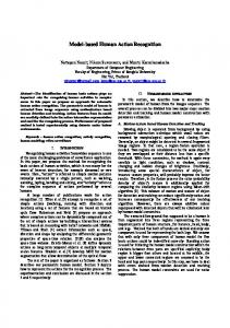
We use the SFM (structure from motion) model to reconstruct the missing trajectories of the occluded joints [27]. Consider a set of 𝑃𝑛 point trajectories extracted from the 𝑛 parts of human body that rigidly moves in 𝑓 frames. By stacking each image trajectory in a single matrix 𝑤𝑛 of 2𝐹×𝑃𝑛 , it is possible to express the global motion, which represents the complete trajectory. We define it as 𝑋1 ⋅ ⋅ ⋅ 𝑋𝑛 󸀠 𝑅1𝑛 𝑡1𝑛 [𝑌 ⋅⋅⋅𝑌 ] [ ][ 𝑛] 𝑤𝑛 = 𝑀𝑛 𝑆𝑛 = [ ... ] [ 1 ], [ 𝑍 ⋅ ⋅ ⋅ 𝑍 1 𝑛] 󸀠 [𝑅𝐹𝑛 𝑡𝐹𝑛 ] [ 1⋅⋅⋅1 ]

(12)

where 𝑀𝑛 is the 2𝐹 × 4 human body motion matrix and 𝑆𝑛 is the human body contour matrix in homogenous coordinates. Each frame-wise element 𝑅𝑓𝑛 , for 𝑓 = 1, . . . , 𝐹, is a 2 × 3 orthographic camera matrix that has to satisfy the metric 𝑇 constraints of the model (i.e., 𝑅𝑓𝑛 𝑅𝑓𝑛 = 𝐼2 × 2 ). The 2-vector 󸀠 𝑡𝐹𝑛 represents the 2D translation of the rigid object (in this paper, we consider the human body as a rigid object). We introduce the registered 𝑤𝑛󸀠 measurement matrix such that 󸀠𝑇 󸀠 𝑤𝑛󸀠 = 𝑤𝑛 − 𝑡󸀠 1󸀠𝑇 𝑃n , where 1𝑃n is a vector of 𝑃𝑛 ones and 𝑡 = 󸀠𝑇 󸀠𝑇 [𝑡1 , . . . , 𝑡𝐹 ]. In the case of missing data due to occlusions, we define the binary mask matrix 𝐺𝑛 of size 2𝐹 × 𝑃𝑛 such that 1 represents a known entry and 0 denotes a missing one. In order to solve the components and thus the SFM problem, the equivalent optimization problem [28] can be defined as 󵄩2 󵄩 Minimize 󵄩󵄩󵄩𝐺𝑛 ⊗ (𝑤𝑛 − 𝑀𝑛 𝑆𝑛 )󵄩󵄩󵄩 , 𝑇 = 𝐼2 × 2 , Subject to 𝑅𝑓𝑛 𝑅𝑓𝑛

𝑓 = 1, . . . , 𝐹.

(13)

Therefore, we can get to make up for the missing point of the trajectory. Figure 1 shows the reconstructed trajectory of the missing point.

4

The Scientific World Journal

4. Feature Representation 4.1. Motion Feature Extraction. The human action can be recognized in terms of hierarchical area model and relative velocity. In this paper, we use optical flow to detect the relative direction and magnitude of environmental motion observed in reference to an observer and also describe the movement of object from current image with respect to the last image. The optical flow [22, 29] equation can be assumed to hold for all pixels within a window centered at 𝑝, the local image flow (velocity) vector (𝑉𝑥 , 𝑉𝑦 ) must be satisfied, and we define some equations as follows: 𝐼𝑥 (𝑠1 ) 𝑉𝑥 + 𝐼𝑦 (𝑠1 ) 𝑉𝑦 = −𝐼𝑡 (𝑠1 ) , (14)

𝐼𝑥 (𝑠𝑑 ) 𝑉𝑥 + 𝐼𝑦 (𝑠𝑑 ) 𝑉𝑦 = −𝐼𝑡 (𝑠𝑑 ) , where 𝑠1 , 𝑠2 , . . . , 𝑠𝑑 are the pixels inside the window and 𝐼𝑥 (𝑠𝑖 ), 𝐼𝑦 (𝑠𝑖 ), and 𝐼𝑡 (𝑠𝑖 ) are the partial derivatives of the image 𝐼 with respect to position 𝑥, 𝑦 and time 𝑡, evaluated at the point 𝑆𝑖 and the current time. These equations can be written in matrix form 𝐴V = 𝑏, where 𝐼𝑥 (𝑠1 ) 𝐼𝑦 (𝑠1 ) ] [ [𝐼𝑥 (𝑠2 ) 𝐼𝑦 (𝑠2 )] ], 𝐴=[ .. ] [ ] [ . (𝑠 ) 𝐼 (𝑠 ) 𝐼 𝑥 𝑛 𝑦 𝑛 ] [

𝑉 V = [ 𝑥] , 𝑉𝑦 (15)

−

𝐹𝑦 =

𝐹𝑦+

−

𝐹𝑦− .

(16)

The motion descriptors of two different frames are compared using a version of the normalized correlation. Suppose the four channels for frame 𝑖 of sequence 𝐴 are 𝑎1 , 𝑎2 , 𝑎3 , 𝑎4 and the four channels for frame 𝑗 of sequence 𝐵 are 𝑏1 , 𝑏2 , 𝑏3 , 𝑏4 ; then the similarity between frame 𝐴 𝑖 and 𝐵𝑖 is 4

max𝜃 {𝑚𝜃 (0, 1) Δ 𝜃 } , min𝜃 {𝑚𝜃 (0, 1) Δ 𝜃 }

(19)

where Δ is the distance of pixels [31], 𝐵 is the binary image of the human body area, 𝑚𝜃 (0, 1) is the region 𝐵 in the perpendicular direction to the parallel lines intersecting the number of lines in group, and Δ 𝜃 is the distance between the scan lines. In this paper, we use the eight search directions as shown in Figure 3. Therefore, distances among search lines, respectively, are Δ 0 = Δ 𝜋/2 = Δ, Δ Δ = Δ arctg2 √2 arctg(1/2)

(20) Δ . √5

In order to implement the silhouette of human body area, a series of steps must be followed: (1) using Gaussian filter to eliminate any noise in video sequence;

The optical flow vector field 𝑉𝑥 is further half-wave rectified into four nonnegative channels. 𝐹𝑥+ , 𝐹𝑥− , 𝐹𝑦+ , 𝐹𝑦− , so that 𝐹𝑥 =

(18)

We assume that this area has a maximum value in the 𝜃 direction. The length of the projection area in the 𝜃+(𝜋/2) direction is defined as the area width:

= Δ (𝜋/2)+arctg(1/2) = Δ (𝜋/2)+arctg2 =

[−𝐼𝑡 (𝑠𝑑 )]

𝐹𝑥− ,

V (𝑖) , ℎ (𝑖)

V (𝑖) = 𝑚𝜃+(𝜋/2) (0, 1) Δ 𝜃+(𝜋/2) .

Δ 𝜋/4 = Δ 3𝜋/4 =

−𝐼𝑡 (𝑠1 ) [−𝐼𝑡 (𝑠2 )] [ ] 𝑏 = [ . ]. [ .. ]

𝐹𝑥+

𝐿=

ℎ (𝑖) =

𝐼𝑥 (𝑠2 ) 𝑉𝑥 + 𝐼𝑦 (𝑠2 ) 𝑉𝑦 = −𝐼𝑡 (𝑠2 ) , .. .

of silhouette in horizontal and vertical are ℎ(𝑖) and V(𝑖), respectively, and their ratio is 𝐿, so we define it as

𝑗+𝑡

𝑆 (𝐴 𝑖 , 𝐵𝑖 ) = ∑ ∑ ∑ 𝑎𝑐𝑖+𝑡 (𝑥, 𝑦) 𝑏𝑏 (𝑥, 𝑦) ,

(17)

𝑡∈𝑇 𝑑=1 𝑥,𝑦∈𝐼

where 𝑇 and 𝐼 are the temporal and spatial extent of the motion descriptors. In this paper, we choose 𝑇 = 20. Therefore, we can obtain the key frames by the frames cluster. Figure 2 depicts results of key-frame extracted by the optical flow. Then, we extract the feature from the key frame. We assume that the overall key frame number is 𝑖, the lengths

(2) using filter to find the edge strength, which estimates the gradient in the 𝑥-direction and the other estimating the gradient in the 𝑦-direction; (3) the direction of the edge is computed using the gradient in the 𝑥 and 𝑦 directions; (4) after the edge directions are known nonmaximum suppression now has to be applied. Nonmaximum suppression is used to trace along the edge in the edge direction and suppress any pixel value (sets it equal to 0) that is not considered to be an edge. This will give a thin line in the output; (5) threshold 𝑇1 is applied to the frames, and an edge has an average strength equal to 𝑇1. Any pixel in the frame that has a value greater than 𝑇1 is presumed to be an edge and is marked as such immediately and then any pixels that are connected to this edge pixel and that have a value. Figure 4 shows the silhouette of human body area. Therefore, we can obtain the body contours by this step and use the optical flow descriptor and 𝐿 descriptor (the ratio of the width and height) to represent the video frames. To construct the codebook, we randomly select a subset from

The Scientific World Journal

5

Walking

Jogging

Running

(a)

15

100 80 60 z 40 20 0 −20 1000 500 y

10

10 z

5

5

z

0

0 −5

−5 −10 10

0

0 −500 −50 x −1000 −100

50

−10 40

5

100

y

0

−5

−10 −10

−5

0

5

10

20 y

x

0

0 −20 −5 x −40 −10

5

10

(b)

Figure 1: Examples of reconstructed 3-D trajectories. Hip rotations for walking, jogging, and running actions in the KTH dataset [30]. (a) It shows original images. (b) It shows reconstructing the missing data of point trajectories.

Boxing

Handclapping

Running

Jogging

Handwaving

Walking

Original image

Key frame

Figure 2: Results of key-frame extracted method.

Figure 3: Eight searching directions in image.

all the frames and compute the affinity matrix on this subset of frames, where each entry in the affinity matrix is the similarity between frame 𝑖 and frame 𝑗 calculated using the normalized correlation described above. Then, we run 𝑘medoid clustering on this affinity matrix to obtain 𝑉 clusters. Code-words are then defined as the centers of the obtained clusters. 4.2. Construct the Codebook. In the end, each video sequence is converted to the “bag of words” representation by replacing

each frame by its corresponding codeword and removing the temporal information. We follow the instruction from statistical text document analysis, and each image is represented as a bag of codewords. Given a training set of images with annotation words, we use the following notation. Each image is a collection of 𝑀 visual feature code-words, denoted as V = {V1 : 𝑀}, where V𝑚 is a unit-basis vector of size 𝑉𝑠 with exactly one nonzero entry representing the index of current visual feature in the visual feature dictionary of size 𝑉𝑠 . Similarly, for one image annotated with 𝑁 words 𝑊 = {𝑤1 : 𝑁}, we denote each word 𝑤𝑛 as a unit-basis vector of size 𝑉𝑡 again with only one taking values 1 and 0 otherwise; here 𝑉𝑡 is the word dictionary size. Therefore, a collection of 𝐷 training image word pairs can be denoted as {V1:𝐷, 𝑊1:𝐷}.

5. Action Classification In order to capture the correlation of topics, we model the hyperparameter of topic prior distribution as multivariate

6

The Scientific World Journal Actions

Bending

Jumping

Walking

Running

The silhouette of human body area

Figure 4: The silhouette of human body area.

𝜇

𝜃

M

Σ

D

z

v

𝜋

y

w

𝛽

N

K

Figure 5: Graphical representation of the variational distribution for CTM.

normal distribution instead of Dirichlet, similar to [29, 32] and the structure topics of dependencies by covariance matrix, and then we use the logistic normal function: 𝑓 (𝜃𝑖 𝑒) = (

exp 𝜃𝑖

∑𝐾 𝑗=1

exp 𝜃𝑗

)

(21)

to project the multivariate normal to topic proportions for each image; here 𝐾 is the topic number. Let {𝜇, Σ} be a 𝐾-dimensional mean and variance matrix from normal distribution, and let topics 𝜋1:𝑘 be 𝐾 multinomials over fixed vocabulary with size 𝑉𝑠 and let 𝛽1:𝐾 be 𝐾 multi-nomials over a fixed text word vocabulary with size 𝑉𝑡 . The CTM generates an image-word pair with 𝑀 image codewords and 𝑁 annotation words [29, 32] from the following generative process: (1) draw topic proportions 𝜃{𝜇, Σ} ∼ 𝑁(𝜇, Σ) (2) for each visual feature V𝑚 , 𝑚 ∈ {1, . . . , 𝑚} (a) draw topic assignment 𝑧𝑚 ∼ Mult(𝑓(𝜃)) (b) draw visual feature V𝑚 ∼ Mult(𝜋𝑧𝑚 ) (3) for each textual word 𝑤𝑛 , 𝑛 ∈ {1, , . . . , 𝑁} (a) draw feature index 𝑦𝑛 ∼ Unif(1, , . . . , 𝑀) (b) draw textual word 𝑤𝑛 ∼ Mult(𝛽𝑧𝑦 ). 𝑛

Firstly, we generate 𝑀 feature V𝑚 from correlated topic proportions 𝜃, conditional on the topic feature multinomial 𝜋, then for each of the 𝑁 text words, one of the 𝑀 features is selected and correspondingly assigned to a text word 𝑤𝑛 , conditional on the topic word multinomial 𝛽. This model is shown as a directed graphical model in Figure 5. From the generative process of CTM, it could be learned that topic correlations are modeled and generated through the covariance matrix Σ of prior multivariate normal distribution. To learn the parameters of CTM that maximizes

the likelihood of training data, we iteratively estimate the model parameters of latent variables. In this paper, the first step is to add and calculate a set of variational parameters to obtain the approximate lower-bound on likelihood of each sample. The latter step is to estimate the model parameters that maximize the log likelihood of the whole training samples. In the graphical representation of CTM in Figure 5, 𝜃 is conditional dependent on the parameter 𝜋, which leads to intractability for computing the log likelihood. The meanfield variational distribution is 𝑀

𝑁

𝑚=1

𝑛=1

𝑞 (𝜃, 𝑧, 𝑦) = 𝑞 (𝜃 | 𝛾, V) ∏ 𝑞 (𝑍𝑚 | 𝜙𝑚 ) ∏𝑞 (𝑦𝑛 | 𝜆 𝑛 ) , (22) where (𝛾, V) is variational mean and variance of normal distribution, 𝜙𝑚 is a variational multinomial over 𝐾 topics, and 𝜆 𝑛 is a variational multinomial over codewords. Let Δ = {𝜇, Σ, 𝜋, 𝛽} denote model parameters; we bound the log-likelihood of an image-annotation pair (V, 𝑤) as follows: log 𝑝 (V, 𝑤 | Δ) = log ∫

𝜃

𝑝 (V, 𝑤, 𝜃, 𝑧, 𝑦 | Δ) 𝑞 (𝜃, 𝑧, 𝑦) 𝑑𝑥 𝑑𝑦 𝑞 (𝜃, 𝑧, 𝑦)

(23)

≥ 𝐸𝑞 [log 𝑝 (V, 𝑤, 𝜃, 𝑧, 𝑦 | Δ)] − 𝐸𝑞 [log 𝑞 (V, 𝑤, 𝜃, 𝑧, 𝑦 | Δ)] = 𝜄 (𝛾, V, 𝜙, 𝜆; Δ) , where 𝐸𝑞 is the expectation according to the variational distribution. Taking the log likelihood function 𝜄(𝛾, V, 𝜙, 𝜆; Δ) as object function, we fit these parameters with coordinate ascent to maximize the object function: 𝜄 = 𝐸𝑞 [log 𝑝 (𝜃 | 𝜇, Σ)] + ∑𝐸𝑞 [log 𝑝 (𝑧𝑚 | 𝜃)] 𝑚

+ 𝐸𝑞 [log 𝑝 (V𝑚 | 𝑧𝑚 , 𝜋)] + ∑𝐸𝑞 [log 𝑝 (𝑦𝑚 | 𝑀)] 𝑚

The Scientific World Journal Walking

Boxing

7 Jogging

Running

Hand waving

Hand clapping

(a)

(b)

(c)

Figure 6: Sample frames from our datasets. The action labels in each dataset are as follows: (a) KTH dataset: walking (a1), jogging (a2), running (a3), boxing (a4), handclapping (a5); (b) Weizmann dataset: running, walking, jumping-jack, waving-two-hands, waving-one-hand, bending; (c) UIUC action dataset: raising two hands (a1), running (a2), clapping (a3), stretching out (a4), and pushing up (a5).

+ 𝐸𝑞 [log 𝑝 (𝑤 | 𝑦𝑚 , 𝑧𝑚 , 𝛽)] − 𝐸𝑞 [log 𝑞 (𝜃 | 𝛾, V)]

We define Δ = {𝜇, Σ, 𝜋, 𝛽}; the overall log likelihood of collection is bounded by

− ∑𝐸𝑞 [log 𝑞 (𝑧𝑚 | 𝜃)] − ∑𝐸𝑞 [log 𝑞 (𝑦𝑚 | 𝜆)] , 𝑚

𝑛

(24) −1 𝑀 𝜕𝜄 (𝛾) = −∑ (𝛾 − 𝜇) + ∑ 𝜙𝑚,1:𝐾 𝜕𝛾 𝑚=1

𝑀 ]2 − ( ) exp (𝛾 + ) , 𝜍 2 ∑−1 𝑖𝑖

]2𝑖

𝜕𝜄 (]𝑖 ) 𝑀 1 =− . − ( ) exp (𝛾 + ) + 2 2 2𝜍 2 𝜕]𝑖 (2]2𝑖 )

(25)

(26)

𝑁

𝑖=1

𝑛=1

𝐷

𝑑=1

𝑑=1

(29)

We maximize the lower boundary of 𝜄, by plugging (23) into (17), and then update model parameters by setting derivation equal zero with respect to each model parameter. The terms containing 𝜋𝑖𝑗 are 𝐷 𝑀𝑑 𝐾 𝑉𝑠

𝑉𝑠

𝑑=1 𝑚=1 𝑖=1 𝑗=1

𝑗=1

𝜄 (𝜋𝑖𝑗 ) = ∑ ∑ ∑ ∑ 𝜙𝑑𝑚𝑖 log 𝜋𝑖,V𝑚 − 𝐶 ( ∑𝜋𝑖𝑗 − 1) . (30) Setting 𝜕𝜄(𝜋𝑖𝑗 )/𝜕𝜋𝑖𝑗 = 0 leads to

Then, we update variational multinomial 𝜙. The terms in 𝜄 with respect to 𝜙𝑚 are 𝐾

𝐷

𝜄 = ∑ log 𝑝 (V𝑑 𝑤𝑑 | Δ) ≥ ∑ 𝜄𝑑 (𝛾𝑑 , V𝑑 , 𝜙𝑑 , 𝜆 𝑑 ; Δ) .

𝐷 𝑀𝑑

𝑗

𝜋𝑖𝑗󸀠 ∝ ∑ ∑ 𝜙𝑑𝑚𝑖 V𝑑𝑚 .

(31)

𝑑=1 𝑚=1

The terms containing 𝛽1:𝐾 are

𝜄 (𝜙𝑚 ) = ∑𝜙𝑚𝑖 (𝛾𝑖 + log 𝜋𝑖,V𝑚 − log 𝜙𝑚𝑖 + ∑ 𝜆 𝑛𝑚 log 𝛽𝑖,𝑤𝑛 ) , (27) 𝑁 𝜕𝜄 (𝜙𝑚𝑖 ) = 𝛾𝑖 + log 𝜋𝑖,V𝑚 + ∑ 𝜆 𝑛𝑚 𝛽𝑖,𝑤𝑛 − log 𝜙𝑚𝑖 + 𝐶, (28) 𝜕𝜙𝑚𝑖 𝑛=1

where ∑𝐾 𝑖=1 𝜙𝑚𝑖 = 1 is the multinomial constrain. 𝐶 is the constant. The full variational inference procedure repeats the updates of (24), (25) until (23); the object function converges. Then, we will obtain the parameter estimation. Given a collection of human action image data with annotation words {V𝑑 , 𝑤𝑑 }𝐷 𝑑=1 , we find the maximum likelihood estimation for parameter {𝜇, Σ, 𝜋, 𝛽}.

𝐷 𝑁𝑑 𝐾 𝑉𝑡 𝑀𝑑

𝜄 (𝛽𝑖,𝑗 ) = ∑ ∑ ∑ ∑ ∑ 𝜙𝑑𝑚𝑖 𝜆 𝑛𝑚 log 𝛽𝑖,𝑤𝑛 𝑑=1 𝑛=1 𝑖=1 𝑗=1 𝑚=1

(32)

𝑉𝑡

− 𝐶 ( ∑𝛽𝑖𝑗 − 1) . 𝑗=1

Setting 𝜕𝜄(𝛽𝑖𝑗 )/𝜕𝛽𝑖𝑗 = 0 leads to 𝐷 𝑁𝑑

𝑗

𝑀𝑑

𝛽𝑖𝑗󸀠 ∝ ∑ ∑ 𝑤𝑑𝑛 ∑ 𝜙𝑑𝑚𝑖 𝜆 𝑑𝑛𝑚 . 𝑑=1 𝑛=1

(33)

𝑚=1

The terms containing 𝜇 are −1 1 𝐷 𝑇 𝜄 (𝜇) = − ( ) ∑ (𝛾𝑑 − 𝜇) ∑ (𝛾𝑑 − 𝜇) . 2 𝑑=1

(34)

8

The Scientific World Journal a1 a2 a3 a4 a5

0.94 0.03 0.02 0.00 0.03 a1

0.03 0.94 0.03 0.00 0.03 a2

0.02 0.07 0.87 0.00 0.08 a3

0.00 0.00 0.00 0.90 0.01 a4

0.00 0.00 0.00 0.25 0.75 a5

Figure 7: Confusion matrix for KTH dataset. a1 a2 a3 a4 a5 a6 a7 a8 a9

1.00 0.02 0.00 0.00 0.03 0.00 0.00 0.00 0.00 a1

0.00 0.98 0.00 0.00 0.03 0.00 0.15 0.00 0.00 a2

0.03 0.01 0.75 0.00 0.00 0.00 0.00 0.03 0.01 a3

0.01 0.08 0.12 1.00 0.01 0.00 0.00 0.01 0.00 a4

0.00 0.00 0.13 0.00 0.75 0.05 0.41 0.00 0.02 a5

0.00 0.00 0.00 0.00 0.00 0.90 0.00 0.12 0.00 a6

0.02 0.00 0.04 0.00 0.31 0.04 0.95 0.00 0.00 a7

0.00 0.00 0.00 0.00 0.00 0.00 0.00 0.98 0.00 a8

0.00 0.00 0.00 0.00 0.20 0.00 0.00 0.00 1.00 a9

Figure 8: Confusion matrix for Weizmann dataset.

Setting 𝜕𝜄(𝜇)/𝜕𝜇 = 0 leads to 𝜇󸀠 = (

1 𝐷 ) ∑𝛾 . 𝐷 𝑑=1 𝑑

(35)

The terms containing Σ are 𝐷 1 1 󵄨 󵄨 𝜄 (Σ) = ∑ {( ) log 󵄨󵄨󵄨󵄨𝜎−1 󵄨󵄨󵄨󵄨 − ( ) Tr [diag (V𝑑2 ) Σ−1 ] 2 2 𝑑=1

6.2. Comparison (36)

1 𝑇 − ( ) (𝛾𝑑 − 𝜇) Σ−1 (𝛾𝑑 − 𝜇)} . 2 Setting 𝜕𝜄(Σ)/𝜕Σ = 0 leads to Σ󸀠 = (

𝑇 1 𝐷 ) ∑ (𝐼 × V𝑑2 + (𝛾𝑑 − 𝜇󸀠 ) (𝛾𝑑 − 𝜇󸀠 ) ) . 𝐷 𝑑=1

(37)

If we obtain variational parameters {𝛾𝑑 , V𝑑 , 𝜙𝑑 , 𝜆 𝑑 , 𝜍𝑑 }𝐷 𝑑=1 for all the training samples, we can update the model parameters {𝜇, Σ, 𝜋, 𝛽} by plugging them into (30), (34), and (36) until the overall likelihood in (28) converges. Therefore, We approximate the conditional distribution of code-words as follows: 𝑀

𝑝 (𝑤 | V) = ∑ ∑𝑞 (𝑧𝑚 | 𝜙𝑚 ) 𝑝 (𝑤 | 𝑧𝑚 , 𝛽) . 𝑚=1 𝑧𝑚

action dataset [30], and the UIUC action dataset [34]. All the experiments are conducted on a Pentium 4 machine with 2 GB of RAM, using the implementation on MATLAB. The dataset and the related experimental results are presented in the following sections. The KTH dataset is provided by Schuldt which contains 2391 video sequences with 25 actors showing six actions. Each action is performed in 4 different scenarios. The WEIZMANN dataset is provided by Blank which contains 93 video sequences showing nine different people, each performing ten actions, such as run, walk, skip, jump-jack, jump-forward-on-two-legs, jump-in-place-ontwo-legs, gallop-sideways, wave-two-hands, wave-one-hand, and bend. The UIUC action dataset is created by the University of Illinois at Urbana-Champaign (UIUC) in 2008 for human activity recognition. The activities are walking, running, jumping, waving, jumping jacks, clapping, jumping from sit up, raising one hand, stretching out, turning, sitting to standing, crawling, pushing up, and standing to sitting. For every dataset, 12 video sequences are taken by four subjects (out of the five) used for training and the remaining three videos for testing. The experiments are repeated five times. The performance of different methods is shown using the average recognition rate. In order to evaluate the performance of action recognition, we report the overall accuracy on three datasets.

(38)

The conditional probability 𝑝(𝑤 | V) can be treated as the predicted confidence score of each annotation word in word vocabulary, given the whole code-words of the unknown human behavior.

6. Experimental Result 6.1. Datasets. We test our algorithm on three datasets: the Weizmann human motion dataset [33], the KTH human

KTH Dataset. It contains six types of human actions (walking, jogging, running, boxing, hand waving, and hand clapping) performed several times by 25 subjects in four different scenarios: outdoors, outdoors with scale variation, outdoors with different clothes, and indoors. Representative frames of this dataset are shown in Figure 6(a). After process of restoring missing coordinate position, we use the proposed method, and the classification results of KTH dataset obtained by this approach are shown in Figure 7 and indicate quite a small number of videos are misclassified, particularly, the actions “running” and “handclapping” which more tend to be confused. The Weizmann Dataset. The Weizmann human action dataset contains 83 video sequences showing nine different people and all performing nine different actions: bending (a1), jumping jack (a2), jumping forward on two legs (a3), jumping in place on two legs (a4), running (a5), galloping sideways (a6), walking (a7), waving one hand (a8), and waving two hands (a9). The figures were tracked and stabilized by using the background subtraction masks that come with this dataset. Some sample frames are shown in Figure 6(b). The classified results achieved by this approach are shown in Figure 8. The UIUC Action Dataset. This dataset consists of 532 high resolution sequences of 14 activities performed by eight actors. The activities are walking, running, jumping, waving, jumping jacks, clapping, jumping from sit-up, raising one

The Scientific World Journal

9

Table 1: Compared with other approaches on KTH dataset. Method The proposed method Zhang and Gong [35] Gong et al. [36] Chang et al. [37]

Average recognition rate (%) 90.60 83.40 89.20 88.03

a1 a2 a3 a4 a5

1.00 0.00 0.03 0.00 0.04 a1

0.00 0.98 0.04 0.13 0.02 a2

0.03 0.00 0.89 0.00 0.00 a3

0.10 0.15 0.00 0.85 0.01 a4

0.00 0.00 0.10 0.04 0.86 a5

Figure 9: Confusion matrix for UIUC dataset.

Table 2: Compared with other approaches on Weizmann dataset. Method The proposed method Zhang and Gong [35] Gong et al. [36] Chang et al. [37]

Average recognition rate (%) 89.20 85.30 86.30 82.10

Table 3: Compared with other approaches on UIUC dataset. Method The proposed method Zhang and Gong [35] Gong et al. [36] Chang et al. [37]

Average recognition rate (%) 93.30 89.70 92.50 91.20

calculated the ratio of the width and height from human silhouette. Finally, we use the topic model of correlated topic model (CTM) to classify and recognize action. Experiments were performed on the KTH, Weizmann, and UIUC action datasets to test and evaluate the proposed method. The compared experiment results showed that the proposed method was more effective than compared methods and better than other approaches [35–37]. Future work will deal with adding complex event detection to the proposed system, involving more complex problems such as dealing with more variable motion, interperson occlusions, and possible appearance similarity of different people and increasing the database size.

Conflict of Interests hand, stretching out, turning, sitting to standing, crawling, pushing up, and standing to sitting. Some sample frames are shown in Figure 6(c). The classified results achieved by this approach are shown in Figure 9. In this paper, we identify jogging, running, walking, and boxing and compare the proposed method with the four state-of-the-art methods in the literature: Zhang and Gong [35], Gong et al. [36], and Chang et al. [37] in three datasets. As shown in Tables 1, 2, and 3, the existing methods, the low recognition accuracy because these action are not only occlusion situation are complex, but also the legs have complex beat, motion and other group actions. The proposed method can overcome these problems, and the recognition accuracy and average accuracy are higher than the comparative method. The experimental results show that the approach proposed in the paper can get satisfactory results and significantly performs better comparing the average accuracy with that in [35–37] because of a practical method adopted in the paper.

7. Conclusions and Future Work In this paper, we proposed an adaptive occlusion action recognition method for human body movement. Our method successfully recognizes without assuming a known and fixed depth order. We have presented the MRF model and SFM model, which estimates the adaptive occlusion state and recovers the important missing parts of objects in a video clip. This paper presents a new method of human self-occlusion behavior recognition, which is based on optical flow and correlated topic model (CTM). Then, we have employed the optical flow motion feature to extract the key frame and

The authors declare that there is no conflict of interests regarding the publication of this paper (such as financial gain).

Acknowledgments This work was supported by the National Natural Science Foundation of China (Grant no. 51278068) and by the Science and Technology Project of Hunan (Grant no. 2013GK3012).

References [1] L.-M. Xia, Q. Wang, and L.-S. Wu, “Vision based behavior prediction of ball carrier in basketball matches,” Journal of Central South University of Technology, vol. 19, no. 8, pp. 2142– 2151, 2012. [2] P. F. Felzenszwalb and D. P. Huttenlocher, “Pictorial structures for object recognition,” International Journal of Computer Vision, vol. 61, no. 1, pp. 55–79, 2005. [3] L. Fei-Fei, R. Fergus, and P. Perona, “One-shot learning of object categories,” IEEE Transactions on Pattern Analysis and Machine Intelligence, vol. 28, no. 4, pp. 594–611, 2006. [4] K. Grauman and T. Darrell, “The pyramid match kernel: discriminative classification with sets of image features,” in Proceedingsof the 10th IEEE International Conference on Computer Vision (ICCV ’05), vol. 2, pp. 1458–1465, October 2005. [5] S. Lazebnik, C. Schmid, and J. Ponce, “A maximum entropy framework for part-based texture and object recognition,” in Proceedings of the 10th IEEE International Conference on Computer Vision (ICCV ’05), vol. 1, pp. 832–838, October 2005. [6] J. Yamato, J. Ohya, and K. Ishii, “Recognizing human action in time-sequential images using hidden Markov model,” in Proceedings of the IEEE Computer Society Conference on Computer Vision and Pattern Recognition (CVPR ’92), 1992.

10 [7] A. F. Bobick and A. D. Wilson, “A state-based approach to the representation and recognition of gesture,” IEEE Transactions on Pattern Analysis and Machine Intelligence, vol. 19, no. 12, pp. 1325–1337, 1997. [8] T. Xiang and S. Gong, “Beyond tracking: modelling activity and understanding behaviour,” International Journal of Computer Vision, vol. 67, no. 1, pp. 21–51, 2006. [9] F. Li and P. Perona, “A bayesian hierarchical model for learning natural scene categories,” in Proceedings of the IEEE Computer Society Conference on Computer Vision and Pattern Recognition (CVPR ’05), vol. 2, pp. 524–531, June 2005. [10] J. Sivic, B. C. Russell, A. A. Efros, A. Zisserman, and W. T. Freeman, “Discovering objects and their location in images,” in Proceedings of the 10th IEEE International Conference on Computer Vision (ICCV ’05), vol. 1, pp. 370–377, October 2005. [11] R. Fergus, L. Fei-Fei, P. Perona, and A. Zisserman, “Learning object categories from Google’s image search,” in Proceedings of the 10th IEEE International Conference on Computer Vision (ICCV ’05), vol. 2, pp. 1816–1823, October 2005. [12] C. Wang, D. Blei, and L. Fei-Fei, “Simultaneous image classification and annotation,” in Proceedings of the IEEE International Conference on Computer Vision and PatternRecognition (CVPR ’09), pp. 1903–1910, June 2009. [13] D. Putthividhya, H. T. Attias, and S. S. Nagarajan, “Topic regression multi-modal Latent Dirichlet Allocation for image annotation,” in Proceedings of the International Conference on Computer Vision and Pattern Recognition (CVPR ’10), pp. 3408– 3415, June 2010. [14] A. Bissacco, M.-H. Yang, and S. Soatto, “Detecting humans via their pose,” in Advances in Neural Information Processing Systems, vol. 19, pp. 169–176, MIT Press, Cambridge, Mass, USA, 2007. [15] J. C. Niebles, H. Wang, and L. Fei-Fei, “Unsupervised learning of human action categories using spatial-temporal words,” International Journal of Computer Vision, vol. 79, no. 3, pp. 299– 318, 2008. [16] S.-F. Wong, T.-K. Kim, and R. Cipolla, “Learning motion categories using both semantic and structural information,” in Proceedings of the IEEE Computer Society Conference on Computer Vision and Pattern Recognition (CVPR ’07), June 2007. [17] K. Guo, P. Ishwar, and J. Konrad, “Action recognition using sparse representation on covariance manifolds of optical flow,” in Proceedings of the 7th IEEE International Conference on Advanced Video and Signal Based (AVSS ’10), pp. 188–195, September 2010. [18] U. Mahbub, H. Imtiaz, and M. A. Rahman Ahad, “An optical flow based approach for action recognition,” in Proceedings of the 14th International Conference on Computer and Information Technology (ICCIT ’11), pp. 646–651, December 2011. [19] H. Imtiaz, U. Mahbub, and M. A. R. Ahad, “Action recognition algorithm based on optical flow and RANSAC in frequency domain,” in Proceedings of the 50th Annual Conference on Society of Instrument and Control Engineers (SICE ’11), pp. 1627– 1631, September 2011. [20] A. Efros, A. Berg, G. Mori, and J. Malik, “Recognizing action at a distance,” in Proceedings of the International Conference on Computer Vision, pp. 726–733, October 2003. [21] M. Ahmad and S. Lee, “Human action recognition using multiview image sequences features,” in Proceedings of the IEEE 7th International Conference on Automatic Face and Gesture Recognition, pp. 523–528, April 2006.

The Scientific World Journal [22] U. Mahbub, H. Imtiaz, and A. Rahman Ahad, “Motion clustering-based action recognition technique using optical flow,” in Proceedings of the IEEE/OSA/IAPR International Conference on Informatics, Electronics and Vision, pp. 919–924, May 2012. [23] R. Chaudhry, A. Ravichandran, G. Hager, and R. Vidal, “Histograms of oriented optical flow and Binet-Cauchy kernels on nonlinear dynamical systems for the recognition of human actions,” in Proceedings of the IEEE Computer Society Conference on Computer Vision and Pattern Recognition Workshops (CVPR ’09), pp. 1932–1939, June 2009. [24] H. Kantz and T. Schreiber, Nonlinear Time Series Analysis, Cambridge University Press, Cambridge, UK, 2003. [25] N.-G. Cho, A. L. Yuille, and S.-W. Lee, “Adaptive occlusion state estimation for human pose tracking under self-occlusions,” Pattern Recognition, vol. 46, no. 3, pp. 649–661, 2013. [26] A. Asthana, M. Delahunty, A. Dhall, and R. Goecke, “Facial performance transfer via deformable models and parametric correspondence,” IEEE Transactions on Visualization and Computer Graphics, vol. 18, no. 9, pp. 1511–1519, 2012. [27] L. Zappella, A. Del Bue, X. Llad´o, and J. Salvi, “Joint estimation of segmentation and structure from motion,” Computer Vision and Image Understanding, vol. 117, no. 2, pp. 113–129, 2013. [28] A. M. Buchanan and A. W. Fitzgibbon, “Damped newton algorithms for matrix factorization with missing data,” in Proceedings of the IEEE Computer Society Conference on Computer Vision and Pattern Recognition (CVPR ’05), pp. 316–322, June 2005. [29] Y. Wang and G. Mori, “Human action recognition by semilatent topic models,” IEEE Transactions on Pattern Analysis and Machine Intelligence, vol. 31, no. 10, pp. 1762–1774, 2009. [30] I. Laptev, Local spatio-temporal image features for motion interpretation [Ph.D. thesis], Computational Vision and Active Perception Laboratory (CVAP), NADA, KTH, Stockholm, Sweden, 2004. [31] H. Liu and M. Wang, “Method for classification of apple surface defect based on digital image processing,” Transactions of the Chinese Society of Agricultural Engineering, vol. 20, no. 6, pp. 138–140, 2004. [32] X. Xu, S. Atsushi, and T. Rin ichiro, “Correlated topic model for image annotation,” in Proceedings of The 19th Korea-Japan Joint Workshop on Frontiers of Computer Vision, pp. 201–208, February 2013. [33] J. Gall and V. Lempitsky, “Class-specific hough forests for object detection,” in Proceedings of the IEEE Computer Society Conference on Computer Vision and Pattern Recognition Workshops (CVPR ’09), pp. 1022–1029, June 2009. [34] D. Tran and A. Sorokin, “Human activity recognition with metric learning,” in Proceedings of the 10th European Conference on Computer Vision (ECCV ’08), pp. 548–561, 2008. [35] J. Zhang and S. Gong, “Action categorization by structural probabilistic latent semantic analysis,” Computer Vision and Image Understanding, vol. 114, no. 8, pp. 857–864, 2010. [36] J. Gong, C. H. Caldas, and C. Gordon, “Learning and classifying actions of construction workers and equipment using Bag-ofVideo-Feature-Words and Bayesian network models,” Advanced Engineering Informatics, vol. 25, no. 4, pp. 771–782, 2011. [37] J.-Y. Chang, J. Shyu, and C. Cho, “Fuzzy rule inference based human activity recognition,” in Proceedings of the IEEE International Conference on Control Applications (CCA ’09), pp. 211–215, Saint Petersburg, Russia, July 2009.