Apr 3, 2015 - We also show the same bound for online convolution conditioned on a new .... Online pattern matching with address errors (L2-rearrangement distance) ...... 17th ACM-SIAM Symp. on Discrete Algorithms, pages 1221â1229.
The complexity of computation in bit streams Rapha¨el Clifford
Markus Jalsenius
Benjamin Sach
arXiv:1504.00834v1 [cs.CC] 3 Apr 2015
Department of Computer Science University of Bristol Bristol, UK
Abstract We revisit the complexity of online computation in the cell probe model. We consider a class of problems where we are first given a fixed pattern or vector F of n symbols and then one symbol arrives at a time in a stream. After each symbol has arrived we must output some function of F and the n-length suffix of the arriving stream. Cell probe bounds of Ω(δ lg n/w) have previously been shown for both convolution and Hamming distance in this setting, where δ is the size of a symbol in bits and w ∈ Ω(lg n) is the cell size in bits. However, when δ is a constant, as it is in many natural situations, these previous results no longer give us non-trivial bounds. We introduce a new lop-sided information transfer proof technique which enables us to prove meaningful lower bounds even for constant size input alphabets. We use our new framework to prove an amortised cell probe lower bound of Ω(lg2 n/(w · lg lg n)) time per arriving bit for an online version of a well studied problem known as pattern matching with address errors. This is the first non-trivial cell probe lower bound for any online problem on bit streams that still holds when the cell sizes are large. We also show the same bound for online convolution conditioned on a new combinatorial conjecture related to Toeplitz matrices.
1
Introduction
We revisit the complexity of online computation in the cell probe model. In recent years there has been considerable progress towards the challenging goal of establishing lower bounds for both static and dynamic data structure problems. A third class of data structure problems, one which falls somewhere between these two classic settings, is online computation in a streaming setting. Here one symbol arrives at a time and a new output must be given after each symbol arrives and before the next symbol is processed. The key conceptual difference to a standard dynamic data structure problem is that although each arriving symbol can be regarded as a new update operation, there is only one type of query which is to output the latest value of some function of the stream. Online pattern matching is particularly suited to study in this setting and cell probe lower bounds have previously been shown for different measures of distance including Hamming distance, inner product/convolution and edit distance [5, 6, 4]. All these 1
previous cell probe lower bounds have relied on only one proof technique, the so-called information transfer technique of Pˇatra¸scu and Demaine [15]. In loose terms the basic idea is as follows. First one defines a random input distribution over updates. Here we regard an arriving symbol as an update and after each update we perform one query which simply returns the latest distance between a predefined pattern and the updated suffix of the stream. Then one has to argue that knowledge of the answers to ` consecutive queries is sufficient to infer at least a constant fraction of the information encoded by ` consecutive updates that occurred in the past. If one can show this is true for all power of two lengths ` and ensure there is no double counting then the resulting lower bound follows by summing over all these power of two lengths. For the most natural cell size w ∈ Ω(lg n), a cell probe lower bound of Ω(δ lg n/w) for both Hamming distance and convolution using this method was shown, where δ is the size of an input symbol, w is the cell size in bits and n is the length of the fixed pattern [5, 6]. When δ = w, there is also a matching upper bound in the cell probe model and so no further progress is possible. However, when the symbol size δ is in fact constant, the best lower bound that is derivable reduces trivially to be constant. This is a particularly unfortunate situation as arguably the most natural setting of parameters is when the input alphabet is of constant size but the cell size is not. To make matters worse, this limitation is neither specific to pattern matching problems nor even to online problems in general. As it is a fundamental feature of the information transfer technique the requirement to have large input alphabets also applies to a wide of dynamic data structure problems for which the information transfer technique has been up to this point the lower bound method of choice. As a result we see the challenge of providing a new proof technique which can meaningfully handle constant sized alphabets as fundamental to the aim of advancing our knowledge of the true complexity of both online and dynamic problems. We introduce a new lop-sided version of the information transfer technique that enables us to give meaningful lower bounds for precisely this setting, that is when δ ∈ O(1) and w ∈ Ω(lg n). Our proof technique will rely on being able to show for specific problems that we need only ` query answers to give at least a constant fraction of the information encoded in ` lg ` updates. We demonstrate our new framework by first by applying it to the well studied online convolution problem. For this problem we give a conditional cell probe lower bound which depends on a new combinatorial conjecture involving Toeplitz matrices. We then show that it is possible to derive an identical but this time unconditional lower bound by applying the lop-sided information transfer technique to a problem called online pattern matching with address errors [2]. This measure of distance arises in pattern matching problems where errors occur not in the content of the data but in the addresses for where the data is stored.
Previous cell probe lower bounds Our bounds hold in a particularly strong computational model, the cell-probe model, introduced originally by Minsky and Papert [12] in a different context and then subse2
quently by Fredman [8] and Yao [17]. In this model, there is a separation between the computing unit and the memory, which is external and consists of a set of cells of w bits each. The computing unit cannot remember any information between operations. Computation is free and the cost is measured only in the number of cell reads or writes (cell-probes). This general view makes the model very strong, subsuming for instance the popular word-RAM model. The first techniques known for establishing dynamic data structure lower bounds had historically been based on the chronogram technique of Fredman and Saks [9] which can at best give bounds of Ω(lg n/ lg lg n). In 2004, Pˇatra¸scu and Demaine gave us the first Ω(lg n) lower bounds for dynamic data structure problems [15]. Their technique is based on information theoretic arguments which also form the basis for the work we present in this paper. Pˇatra¸scu and Demaine also presented ideas which allowed them to express more refined lower bounds such as trade-offs between updates and queries of dynamic data structures. For a list of data structure problems and their lower bounds using these and related techniques, see for example [13]. More recently, a further breakthrough was made by Larsen who showed lower bounds of roughly Ω((lg n/ lg lg n)2 ) time per operation for dynamic weighted range counting problem and polynomial evaluation [10, 11]. These lower bounds remain the state of the art for any dynamic structure problem to this day.
1.1
Our Results
The lop-sided information transfer technique In the standard formulation of the information transfer technique of Demaine and Pˇatra¸scu [14], adjacent time intervals are considered and the information that is transferred from the operations in one interval of power of two length ` to the next interval of the same length is studied. It is sufficient to prove that a lower bound can be given for the information transfer which applies to all consecutive intervals of power of two length. Conceptually a balanced tree on n leaves over the time axis is constructed which is known as the information transfer tree. An internal node v is associated with the times t0 , t1 and t2 such that the two intervals [t0 , t1 ] and [t1 + 1, t2 ] span the left subtree and the right subtree of v, respectively. By summing over the information transfer at each node v the final lower bound is derived. In order to show a cell probe lower bound for bit streams, we will need to give lower bounds for the information transferred from intervals of time [t0 , t1 ] to later intervals [t2 , t3 ] which are shorter than the first intervals. In particular we will want to argue about intervals of length ` lg ` and ` respectively. However, making the interval lengths lop-sided requires us to abandon the information transfer tree and indeed almost all of the previous proof technique. We will instead place gaps in time between the end of one interval and the start of another and argue carefully both that not too much of the information can be lost in these gaps and that we can still sum the information transfer over a sufficient number of distinct interval lengths without too much double counting. Our hope is that this new technique will lead to a new class of cell probe lower bounds which could not be proved with existing methods.
3
Online convolution In the online convolution problem we are given a fixed vector F ∈ {0, 1}n and a stream that arrives one bit at a time. After each bit arrives we must output the inner product between F and a vector formed from the most recent n-length suffix of the stream. At the heart of our lower bound we need to show that we can recover Ω(` lg `) bits of information of a contiguous subarray of the stream of length ` lg `. However, because the inputs are binary and to avoid a trivial lower bound, we must do so using only ` outputs. As we need to achieve this for a large number distinct values of ` simultaneously, the fixed vector F we design for the online convolution problem has a carefully designed recursive structure. However even having overcome this hurdle, there is still the challenge of showing that for each separate value `, the information from successive outputs does not have too large an overlap. A complete resolution to this question seems non-trivial but in Section 4 we present a new combinatorial conjecture related to Toeplitz matrices, which if true, provides the desired lower bound. As a result we get the following lower bound for online convolution in a bit stream: Theorem 1 (Online convolution). Assuming Conjecture 1, in the cell-probe model with w ∈ Ω(lg n) bits per cell, for any randomised algorithm solving the online convolution problem on binary inputs there exist instances such that the expected amortised time per arriving value is � � lg2 n . Ω w · lg lg n Online pattern matching with address errors (L2 -rearrangement distance) As our second example we give an explicit distance function for which we can now obtain the first unconditional online lower bound for symbol size δ = 1. We consider a problem setting known as pattern matching with address errors and in particular the L2 rearrangement distance as defined in [2]. Consider two strings two strings S1 and S2 both of length n where S2 is a permutation of S1 . Now consider the set of permutations Π so that for all π ∈PΠ, S1 [π(0), . . . , π(n − 1)] = S2 . The L2 -rearrangement distance is defined n−1 to be minπ∈Π j=0 |j − π(j)|2 . If Π is empty, that is S2 is in fact not a permutation of S1 , then the L2 -rearrangement distance is defined to be ∞. When considered as an offline problem, for a text of length 2n and a pattern of length n, Amir et al. showed that the L2 -rearrangement distance between the pattern and every n-length substring of the text could be computed in O(n lg n) time [2]. In the online L2 -rearrangement problem we are given a fixed pattern F ∈ {0, 1}n and the stream arrives one bit at a time. After each bit arrives we must output the L2 -rearrangement distance between F and the most recent n-length suffix of the stream. As before we need to recover Ω(` lg `) bits of information of a contiguous sub-array of the stream of length ` lg `. Our technique allows us to recover Ω(lg n) distinct bits of stream from each output. This is achieved by constructing F and carefully choosing a highly structured random input distribution for the incoming stream in such a way that the contributions to the output from different regions of the stream have different magnitudes. We can then use the result to extract distinct information about the stream from different parts of each output. 4
Using this approach we get the following cell probe lower bound: Theorem 2 (Online L2 -rearrangement). In the cell-probe model with w ∈ Ω(lg n) bits per cell, for any randomised algorithm solving the online L2 -rearrangement distance problem on binary inputs there exist instances such that the expected amortised time per arriving value is � � lg2 n Ω . w · lg lg n
2
Lop-sided information transfer
We will define the concept of information transfer, a particular set of cells probed by the algorithm, and explain how a bound on the size of the information transfer can be used when proving the overall lower bounds of Theorems 1 and 2. All logarithms are in base two.
2.1
Notation for the online problems
The define some notation for our online problems. There is a fixed array F ∈ {0, 1}n of length n and an array S ∈ {0, 1}n of length n, referred to as the stream. We maintain S subject to an update operation u p dat e(x) which takes a value x ∈ {0, 1}, modifies S by appending x to the right of the rightmost component S[n − 1] and removing the leftmost component S[0], and then outputs the inner product of F and S, that is P (F [i] · S[i]), or alternatively the L2 -rearrangement distance, depending on which i∈[n] problem we are currently considering. We let U ∈ {0, 1}n denote the update array which describes a sequence of n u p dat e operations. That is, for each t ∈ [n], the operation u p dat e(U [t]) is performed. We will usually refer to t as the arrival of the value U [t]. Observe that just after arrival t, the values U [t + 1, n − 1] are still not known to the algorithm. Finally, we let the n-length array A denote the outputs such that for t ∈ [n], A[t] is the output of u p dat e(U [t]).
2.2
Hard distributions
Our lower bound holds for any randomised algorithm on its worst case input. This will be achieved by applying Yao’s minimax principle [16]. We develop a lower bound that holds for any deterministic algorithm on some random input. The basic approach is as follows: we devise a fixed array F and describe a probability distribution for U , the n new values arriving in the stream S. We then obtain a lower bound on the expected running time over the arrivals in U that holds for any deterministic algorithm. Due to the minimax principle, the same lower bound must then also hold for any randomised algorithm on its own worst case input. The amortised bound per arriving value is obtained by dividing by n. From this point onwards we consider an arbitrary deterministic algorithm running with some fixed array F on a random input of n values. The algorithm may depend 5
on F . We refer to the choice of F and distribution for U as a hard distribution since it used to show a lower bound.
2.3
Two intervals and a gap
In order to define the concept of information transfer from one interval of arriving values in the stream to another interval of arriving values, we first define the set L which contains the interval lengths that we will consider. The purpose of the next few definitions will be clear once we define information transfer in the next section. We let � � n lg n o 1/4 2i L = n · (lg n) . i ∈ 0, 1, 2, . . . , 4 lg lg n To avoid cluttering the presentation with floors and ceilings, we assume throughout that the value of n is such that any division or power nicely yields an integer. Whenever it is impossible to obtain an integer we assume that suitable floors or ceilings are used. In particular, L contains only integers. For ` ∈ L and t ∈ [n/2] we define the following four values: t0 = t, t1 = t0 + ` lg ` − 1, 4` t2 = t1 + + 1, lg n t3 = t2 + ` − 1. The values t0 , t1 , t2 and t3 are indeed functions of ` and t but for brevity we will often write just t0 instead of t0 (`, t), and so on, whenever the parameters ` and t are obvious from context. The four values define the three intervals [t0 , t1 ], [t1 + 1, t2 − 1] and [t2 , t3 ], referred to as the first interval, the gap and the second interval, respectively. Whenever there is a risk of ambiguity of which parameters the intervals are based on, we may specify what ` and t they are associated with. Before we explain the purpose of the intervals we will highlight some of their properties. First observe that the intervals are disjoint and the gap has length 4`/ lg n. The first interval has length ` lg ` and starts at t, where t is always in the first half of the interval [0, n − 1]. The second interval has length `, hence is a log-factor shorter than the first interval. All intervals are contained in [0, n − 1]. To see this we need to verify that t3 6 n − 1 for any choice of ` ∈ L and t ∈ [n/2]. The largest value in L is 2 lg n
n1/4 · (lg n) 4 lg lg n = n3/4 . Thus, the largest possible value of t3 , obtained with ` = n3/4 and t = n/2 − 1, is ! �n � � � � � 3/4 4n − 1 + n3/4 · lg n3/4 − 1 + + 1 + n3/4 − 1 2 lg n n 6 + 1 + n3/4 (lg n3/4 + 5) < n, 2 6
whenever n is sufficiently large. Lastly, suppose that `0 ∈ L is one size larger than ` ∈ L, that is `0 = ` · (lg n)2 . For `0 the length of the gap is 4`0 / lg n, which so big that it spans the length of both intervals plus the gap associated with `. To see this, observe that for sufficiently large n, 4` +1+`−1+1 lg n 4` (lg n)2 ` 4`0 6 2` lg n + 6 2` lg n + = 3` lg n 6 . lg n lg n lg n
t3 (`, t) − t0 (`, t) + 1 = ` lg ` − 1 +
2.4
Information transfer over gaps
Towards the definition of information transfer, we define, for ` ∈ L and t ∈ [n/2], the subarray U`,t = U [t0 , . . . , t1 ] to represent the ` lg ` values arriving in the stream during the first interval. We define the subarray A`,t = A[t2 , . . . , t3 ] to represent the ` outputs e`,t to be the concatenation of U [0, (t0 − 1)] during the second interval. Lastly we define U e`,t contains all values of U except for those in U`,t . and U [(t1 + 1), (n − 1)]. That is, U For ` ∈ L and t ∈ [n/2] we first define the information transfer to the gap, denoted G`,t , to be the set of memory cells c such that c is probed during the first interval [t0 , t1 ] of arriving values and also probed during the arrivals of the values U [t1 + 1, t2 − 1] in the gap. Similarly we define the information transfer to the second interval, or simply the information transfer, denoted I`,t , to be the set of memory cells c such that c is probed during the first interval [t0 , t1 ] of arriving symbols and also probed during the arrivals of symbols in the second interval [t2 , t3 ] but not in the gap. That is, any cell c ∈ G`,t cannot also be contained in the information transfer I`,t . The cells in the information transfer I`,t may contain information about the values in U`,t that the algorithm uses in order to correctly produce the outputs A`,t . However, since cells that are probed in the gap are not included in the information transfer, the information transfer might not contain all the information about the values in U`,t that the algorithm uses while outputting A`,t . In all previous work on lower bounds where the information transfer technique is used, the two intervals had no gap between them, hence the information transfer I`,t contained all the information about the updates in U`,t necessary for computing A`,t . Further, in all previous work, the two intervals always had the same length. We will see that the introduction of a gap and skewed interval lengths enable us to provide non-trivial lower bounds for small inputs with large cell sizes. We will see that the gap is small enough that a sufficiently large portion of the information about U`,t has to be fetched from cells in the information transfer I`,t . Since cells in the information transfer are by definition probed at some point by the algorithm, we can use I`,t to measure, or at least lower bound, the number of cell probes. As a shorthand we let I`,t = |I`,t | denote the size of the information transfer I`,t . Similarly we let G`,t = |G`,t | denote the size of the information transfer to the gap. By adding up the sizes I`,t of the information transfers over all ` ∈ L and certain values of t ∈ [n/2], we get a lower bound on the total number of cells probed by the algorithm during the n arriving values in U . The choice of the values t is crucial as we do not want 7
to over-count the number of cell probes. In the next two lemmas we will deal with the potential danger of over-counting. For a cell c ∈ I`,t , we write the probe of c with respect to I`,t to refer to the first probe of c during the arrivals in the second interval. These are the probes of the cells in the information transfer that we count. Lemma 1. For any ` ∈ L and t, t0 ∈ [n/2] such that |t − t0 | > `, if a cell c is in both I`,t and I`,t0 then the probe of c with respect to I`,t and the probe of c with respect I`0 ,t0 are distinct. Proof. Since t and t0 are at least ` apart, the second intervals associated with t and t0 , respectively, must be disjoint. Hence the probe of c with respect to I`,t and the probe of c with respect I`,t0 must be distinct. From the previous lemma we know that there is no risk of over-counting cell probes of a cell over information transfers I`,t under a fixed value of ` ∈ L, as long as no two values of t are closer than `. In the next lemma we consider information transfers under different values of ` ∈ L. 6 `0 , and any t, t0 ∈ [n/2], if a cell c is in both Lemma 2. For any `, `0 ∈ L such that ` = I`,t and I`0 ,t0 then the probe of c with respect to I`,t and the probe of c with respect I`0 ,t0 must be distinct. Proof. Let p be the probe of c with respect to I`,t , and let p0 be the probe of c with respect I`0 ,t0 . We will show that p 6= p0 . Suppose without loss of generality that ` < `0 . From the properties of the intervals that were given in the previous section we know that the length of the gap associated with `0 is larger than the sum of lengths of the first interval, the gap and the second interval associated with `. Suppose for contradiction that p = p0 . By definition of I`,t , the cell c is probed also in the first interval associated with `. Let pfirst denote any such cell probe. Because the gap associated with `0 is so large, pfirst must take place either in the second interval or the gap associated with `0 . If pfirst is in the gap, then c cannot be in I`0 ,t0 . If pfirst is in the second interval then p0 cannot equal p. In order to lower bound the total number of cell probes performed by the algorithm over the n arrivals in U we will define, for each ` ∈ L, a set T` ⊆ [n/2] of arrivals, such that for any distinct t, t0 ∈ T` , |t − t0 | > `. It then follows from Lemmas 1 and 2 that XX I`,t `∈L t∈T`
is a lower bound on the number of cell probes. Our goal is to lower bound the expected value of this double-sum. The exact definition of T` will be given in Section 3.3 once we have introduced relevant notation.
8
3
Proving the lower bound
In this section we give the overall proof for the lower bounds of Theorems 1 and 2. Let e`,t is fixed but the values in U`,t are drawn at ` ∈ L and let t ∈ [n/2]. Suppose that U e`,t . random in accordance with the distribution for U , conditioned on the fixed value of U This induces a distribution for the outputs A`,t . We want to show that if the entropy e`,t , then the information transfer I`,t is large, of A`,t is large, conditioned on the fixed U since only the variation in the inputs U`,t can alter the outputs A`,t . We will soon make this claim more precise.
3.1
Upper bound on the entropy
e`,t = u e`,t . We write H(A`,t | U e`,t ) to denote the entropy of A`,t conditioned on fixed U e`,t = u Towards showing that high conditional entropy H(A`,t | U e`,t ) implies large information transfer we use the information transfer I`,t and the information transfer to the gap, G`,t , to describe an encoding of the outputs A`,t . The following lemma gives a direct relationship between I`,t + G`,t and the entropy. A marginally simpler version of the lemma, stated with different notation, was first given in [15] under the absence of gaps. Lemma 3. Under the assumption that the address of any cell can be specified in w bits, for any ` ∈ L and t ∈ [n/2], the entropy e`,t = u e`,t = u H(A`,t | U e`,t ) 6 2w + 2w · E[I`,t + G`,t | U e`,t ]. e`,t is an upper bound on Proof. The expected length of any encoding of A`,t under fixed U the conditional entropy of A`,t . We use the information transfer I`,t and the information transfer to the gap, G`,t , to define an encoding of A`,t in the following way. For every cell c ∈ I`,t ∪ G`,t we store the address of c, which takes at most w bits under the assumption that a cell can hold the address of any cell in memory. We also store the contents of c that it holds at the very end of the first interval, just before the beginning of the gap. The contents of c is specified with w bits. In total this requires 2w · (I`,t + G`,t ) bits. e`,t as part of We will use the algorithm, which is fixed, and the fixed values u e`,t of U the decoder to obtain A`,t from the encoding. Since the encoding is of variable length we also store the size I`,t of the information transfer and the size G`,t of the information transfer to the gap. This requires at most 2w additional bits. In order to prove that the described encoding of A`,t is valid we now describe how to e`,t from the first arrival decode it. First we simulate the algorithm on the fixed input U U [0] until just before the first interval when the first value in U`,t arrives. We then skip over all inputs in U`,t and resume simulating the algorithm from the beginning of the gap, that is when the value U [t1 + 1] arrives. We simulate the algorithm over the arrivals in the gap and the second interval until all values in A`,t have been outputted. For every cell being read, we check if it is contained in either the information transfer I`,t or the information transfer to the gap G`,t by looking up its address in the encoding. If the address is found then the contents of the cell is fetched from the encoding. If not, its e`,t . contents is available from simulating the algorithm on the fixed inputs U 9
3.2
Lower bounds on entropy
Lemma 3 above provides a direct way to obtain a lower bound on the expected value of e`,t = u I`,t + G`,t if given a lower bound on the conditional entropy H(A`,t | U e`,t ). In the next two lemmas we provide such entropy lower bounds for L2 -rearrangement distance and convolution. Lemma 4. Assuming Conjecture 1, for the convolution problem there exists a real constant κ > 0 and, for any n, a fixed array F ∈ {0, 1}n such that for all ` ∈ L and t ∈ [n/2], when U is chosen uniformly at random from {0, 1}n then e`,t = u H(A`,t | U e`,t ) > κ · ` · lg n, for any fixed u e`,t . Lemma 5. For the L2 -rearrangement distance problem there exists a real constant κ > 0 and, for any n, a fixed array F ∈ {0, 1}n such that for all ` ∈ L and all t ∈ [n/2] such n that t mod 4 = 0, when U is chosen uniformly at random from {0101, 1010} 4 then e`,t = u H(A`,t | U e`,t ) > κ · ` · lg n, for any fixed u e`,t . The proof of Lemma 4 is deferred to Section 4 and hinges on a conjecture relating to Toeplitz matrices. The proof of Lemma 5 is deferred to Section 5. Before we proceed with the lower bound on the information transfer we make a short remark on the bounds that these lemmas give. Observe that the maximum conditional entropy of A`,t is bounded by the entropy of U`,t , which is O(` lg `) since the length of the first interval is ` lg `. Recall also that the values in L range from n1/4 to n3/4 . Thus, for a constant κ, both entropy lower bounds are tight up to a multiplicative constant factor.
3.3
A lower bound on the information transfer and quick gaps
In this section we prove our main lower bound results. In order to fix ideas we do this for the L2 -rearrangement problem, given in Theorem 2. As a result we assume that κ is the constant and F is the fixed array of Lemma 4, and that U is chosen uniformly at random from {0, 1}n . Theorem 1 which gives our main lower bound result for online convolution follows via exactly the same argument but with Lemma 4 replaced by Lemma 5. By combining the upper and lower bounds on the conditional entropy from Lemmas 3 and 5 we have that there is a hard distribution and a real constant κ > 0 for the convolution problem such that κ · ` · lg n e`,t = u E[I`,t + G`,t | U e`,t ] > −1 2w e`,t under for any u e`,t . We may remove the conditioning by taking expectation over U random U . Thus, κ · ` · lg n E[I`,t + G`,t ] > − 1, 2w 10
or equivalently
κ · ` · lg n − 1 − E[G`,t ]. 2w Recall that our goal is to lower bound XX XX E I`,t = E [I`,t ] , E[I`,t ] >
`∈L t∈T`
(1)
`∈L t∈T`
where is T` contains suitable values of t. Using Inequality (1) above would immediately provide such a lower bound, however, there is an imminent risk that the negative terms of E[G`,t ] could devalue such a bound into something trivially small. Now, for this to happen, the algorithm must perform sufficiently many cell probes in the gap. Since the length of the gap is considerably shorter than the second interval, a cap on the worst-case number of cell probes per arriving value would certainly ensure that E[G`,t ] stays small, but as we want an amortised lower bound we need something more refined. The answer lies in how we define T` . We discuss this next. For ` ∈ L and f ∈ [`] we first define the set T`,f ⊆ [n] of arrivals to be n no . T`,f = f + i` i ∈ {0, 1, 2, . . . } and f + i` 6 2 The values in T`,f are evenly spread out with distance `, starting at f . We may think of f as the offset of the sequence of values in T`,f . The largest value in the set is no more than n/2. We will define the set T` to equal a subset of one of the sets T`,f for some f . More precisely, we will show that there must exist an offset f such that at least half of the values t ∈ T`,f have the property that the time spent in the gap associated with ` and t is small enough to ensure that the information transfer to the gap is small. We begin with some definitions. Definition 1 (Quick gaps and sets). For any ` ∈ L and t ∈ [n/2] we say that the gap associated with ` and t is quick if the expected number of cell probes during the arrivals in the gap is no more than κ · ` · lg n , 4w where κ is the constant from Lemma 4. Further, for any f ∈ [`] we say that the set T`,f is quick if, for at least half of all t ∈ T`,f , the gap associated with ` and t is quick. The next lemma says that for sufficiently fast algorithms there is always an offset f such that T`,f is quick. Lemma 6. Suppose that the expected total number of cell probes over the n arrivals in U is less than κ · n · lg2 n . 32w Then, for any ` ∈ L, there is an f ∈ [`] such that T`,f is quick. 11
Proof. In accordance with the lemma, suppose that the expected total number of cell probes over the n arrivals in U is less than κn(lg2 n)/(32w). For contradiction, suppose that there is no f ∈ [`] such that T`,f is quick. We will show that the expected number of cell probes over the n arrivals must then be at least κn(lg2 n)/(32w). For any f ∈ [`], let Rf ⊆ [n] be the union of all arrivals that belong to a gap associated with ` and any t ∈ T`,f . Let Pf be the number of cell probes performed by the algorithm over the arrivals in Rf . Thus, for any set T`,f that is not quick we have by linearity of expectation E [Pf ] >
|T`,f | κ · ` · lg n n/2 κ · ` · lg n κ · n · lg n · = · = . 2 4w 2` 4w 8w
Let the set of offsets � F=
4` i· lg n
�� � i ∈ lg n ⊆ [`]. 4
The values in F are spread out with distance 4`/ lg n, which equals the gap length. Thus, for any two distinct f, f 0 ∈ F, the sets Rf and Rf 0 are disjoint. We therefore P have that the total running time over all n arrivals in U must be lower bounded by f ∈F Pf . Under the assumption that no T`,f is quick, we have that the expected total running time is at least X X κ · n · lg n lg n κ · n · lg n κ · n · lg2 n E Pf = E [Pf ] > |F| · = · = , 8w 4 8w 32w f ∈F
f ∈F
which is the contradiction we wanted. Thus, under the assumption that the running time over the n arrivals in U is less than κn(lg2 n)/(32w) there must be an f ∈ [`] such that T`,f is quick. We now proceed under the assumption that the expected running time over the n arrivals in U is less than κn(lg2 n)/(32w). If this is not the case then we have already established the lower bound of Theorem 1. Let f be a value in [`] such that T`,f is a quick set. Such an f exists due to Lemma 6. We now let T` ⊆ T`,f be the set of all t ∈ T`,f for which the gap associated with ` and t is quick. Hence |T` | > |T`,f |/2 = n/(4`). Since G`,t cannot be larger than the number of cell probes in the gap, we have by the definition of a quick gap that for any t ∈ T` , E [G`,t ] 6
κ · ` · lg n . 4w
Using the above inequality together with Inequality (1) we can finally provide a non-trivial
12
lower bound on the sum of the information transfers: � X X � κ · ` · lg n XX E [I`,t ] > − 1 − E[G`,t ] 2w `∈L t∈T` `∈L t∈T` � � X X κ · ` · lg n κ · ` · lg n −1− > 2w 4w `∈L t∈T`
κ · lg n X X κ · lg n X κ · lg n X � n � > ` > (|T` | · `) > ·` 5w 5w 5w 4` `∈L t∈T` `∈L `∈L � � κ · n · lg n κ · n · lg n lg n n · lg2 n . = · |L| > · ∈ Θ 20w 20w 4 lg lg n w · lg lg n By Lemmas 1 and 2 this lower bound is also a bound on the expected total number of cell probes performed by the algorithm over the n arrivals in U . By Yao’s minimax principle, as discussed in Section 2.2, this implies that any randomised algorithm on its worst case input has the same lower bound on its expected running time. The amortised time per arriving value is obtained by dividing the running time by n. This concludes the proofs of Theorem 2 and 1 .
4
The hard distribution for convolution
In this section we prove Lemma 4, which says that assuming Conjecture 1 holds, there exists a real constant κ > 0 and a fixed array F ∈ {0, 1}n such that for all ` ∈ L and t ∈ [n/2], when U is chosen uniformly at random from {0, 1}n then the conditional entropy of the outputs A`,t is e`,t = u H(A`,t | U e`,t ) > κ · ` · lg n, for any fixed u e`,t . We begin by discussing the fixed array F .
4.1
The array F
For each ` ∈ L there is a subarray of F of length ` lg ` + ` − 1. Each such subarray, which we denote F` , is at distance 4`/ lg n + 1 from the right-hand end of F , which is one more than the length of the gap associated with `. Figure 1 illustrates two subarrays F` and F`0 , where `, `0 ∈ L and ` < `0 . By the properties discussed in Section 2.3 we know that the length of the gap associated with `0 is larger than the length of F` plus the length of the gap associated with `. Hence there is no overlap between the subarrays F` and F`0 . Given any of the subarrays F` and an array U` of length ` lg `, we write F` ⊗ U` to denote the `-length array that consists of all inner products between U` and every substring of F` . More precisely, for i ∈ [`] the i-th component of F` ⊗ U` is X � (F` ⊗ U` )[i] = F` [i + j] · U` [j] . j∈[` lg `]
13
4`0 log n
F`0
F
+1 F` 4` log n
+1
Figure 1: Two subarrays F` and F`0 of F . There is never an overlap between any two such subarrays. ` log ` + ` − 1 F` U` ` log ` `
Figure 2: The `-length array F` ⊗ U` contains the inner products of U` and corresponding subarrays of F` as U` slides along F` . As Figure 2 shows we may think of F` ⊗ U` as the inner products of U` and its aligned subarray of F` as U` slides along F` . We can show that there exist subarrays F` such that the entropy of F` ⊗ U` is high when U` is drawn uniformly at random from {0, 1}` lg ` . Observe that the entropy of F` ⊗ U` is upper bounded by the entropy of U` , which is exactly ` lg `. The proof of the next lemma is based on a conjecture that we describe shortly. Lemma 7. There exists a real constant ε > 0 such that for all n and ` ∈ L there is a subarray F` for which the entropy of F` ⊗ U` is at least ε · ` lg ` when U` is drawn uniformly at random from {0, 1}` lg ` . In order to finish the description of the array F we choose each subarray F` such that the entropy of F` ⊗ U` is at least ε · ` lg ` when U` is drawn uniformly at random from {0, 1}` lg ` , where ε is the constant of Lemma 7. Any element of F that is not part of any of the subarrays F` is chosen arbitrarily. This concludes the description of the array F .
4.2
Proving the entropy lower bound
We are now ready to prove Lemma 4, that is lower bound the conditional entropy of A`,t . Proof of Lemma 4. Let F be the array described above and let U be drawn uniformly e`,t , at random from {0, 1}n . Let ` ∈ L and t ∈ [n/2]. Thus, conditioned on any fixed U ` lg ` the distribution of U`,t is uniform on {0, 1} . Recall that U`,t arrives in the stream between arrival t0 and t1 , after which 4`/ lg n values arrive in the gap. Thus, at the beginning of the second interval, at arrival t2 , U`,t is aligned with the (` lg `)-length suffix of the subarray F` of F . Over the ` arrivals in the second interval, U`,t slide along F` similarly to Figure 2 (only in reversed direction 14
e`,t are fixed, the outputs A`,t uniquely of what the diagram shows). Since all values in U specify F` ⊗ U`,t . Thus, by Lemma 7, the conditional entropy ε e`,t = u H(A`,t | U e`,t ) > ε · ` · lg `, > · ` · lg n, 4 since ` > n1/4 . By setting the constant κ to ε/4 we have proved Lemma 4. The last piece remaining is the proof of Lemma 7. This proof is based on a conjecture which we state as follows. Recall that a Toeplitz matrix (or upside-down Hankel matrix) is constant on each descending diagonal from left to right. Conjecture 1. There exist two positive real constants α 6 1 and γ 6 1 such that for any h there is a (0, 1)-Toeplitz matrix M of height h and width α · h lg h with the property that the entropy of the product M v is at least γ · h lg h, where v is a column vector of length α · h lg h whose elements are chosen independently and uniformly at random from {0, 1}. This conjecture might at first seem surprising as the matrix is non-square. However, an essentially equivalent statement was shown to be true for general (0, 1)-matrices in 1974 by Erd˝os and Spencer [7]. Moreover, even stronger statements for general (0, 1)matrices form the basis of the well studied “Coin Weighing Problem with a Spring Scale” (see [3] and references therein). We will now show how to prove Lemma 7 using the conjecture. Proof of Lemma 7 (assuming Conjecture 1). Let α and γ be the two constants in Conjecture 1. Let h = ` and let M be a (0, 1)-Toeplitz matrix of height ` and width α · ` lg ` with the property of Conjecture 1. We now define a new matrix M` of height ` and width ` lg ` such that the submatrix of M` that spans the first α · ` lg ` columns equals M . Remaining elements of M` are filled in arbitrarily from the set {0, 1} so that M` becomes Toeplitz. Let v` be a random column vector of length ` lg ` such that the first α · ` lg ` elements are chosen independently and uniformly from {0, 1}. The remaining elements are fixed arbitrarily. By Conjecture 1 we have that the entropy of M` v` is at least γ · ` lg `. Thus, if we instead pick all elements of v` independently and uniformly at random from {0, 1} then the conditional entropy of M` v` , conditioned on all but the first α · ` lg ` elements, is at least γ · ` lg `. Hence the entropy of M` v` is also at least γ · ` lg `. Now, since M` is Toeplitz we have that the first column and the first row of M` define the entire matrix. These ` + ` lg ` − 1 elements can be represented with an array F` of length ` + ` lg ` − 1 such that F` ⊗ v` = M` v` , where we abuse notation slightly. In other words, the elements of the product M` v` correspond exactly to the inner products obtained by sliding U` , where U` is the array version of the column vector v` , along F` . Thus, the entropy of F` ⊗ U` is at least γ · ` lg `. We may therefore set the constant ε in the statement of the lemma to equal the constant γ of Conjecture 1. This concludes the proof of Lemma 7.
15
5
The hard distribution for L2 -rearrangement
In this section we prove Lemma 5 which says that there exists a real constant κ > 0 and a fixed array F ∈ {0, 1}n such that for all ` ∈ L and all t ∈ [n/4] such that t mod 4 = 0, n when U is chosen uniformly at random from {0101, 1010} 4 then the conditional entropy e`,t = u of the outputs A`,t is H(A`,t | U e`,t ) > κ · ` · lg n for any fixed u e`,t . We begin by discussing the fixed array F .
5.1
The array F
As for the convolution problem, for each ` ∈ L there is a subarray of F of length ` lg ` + `. Each such subarray, which we denote F` , is at distance 4`/ lg n + 1 from the right-hand end of F . This is the same high-level structure as for the convolution problem and so again, there is no overlap between the subarrays F` and F`0 and further, Figure 1 in Section 2.3 is accurate here too. Given any of the subarrays F` and an array U` of length (` lg `), we write F` U` to denote the (`/4)-length array that consists of the L2 -rearrangement distances between U` and every fourth (` lg `)-length substring of F` . More precisely, for 4i ∈ [`], the value of F` U` [i] is the L2 -rearrangement distance between F` [4i, 4i + ` lg ` − 1] and U` . Our main focus in this section is on proving Lemma 8 which can be seen as an analogue of Lemma 5 for a fixed length of `: Lemma 8. There exists a real constant ε > 0 such that for all n and ` ∈ L there is a subarray F` for which the entropy of F` U` is at least ε · ` lg ` when U` is drawn ` uniformly at random from {0101, 1010} 4 lg ` . F` contains an equal number of 0s and 1s. In order to finish the description of the array F we choose each subarray F` in accordance with Lemma 8. Any region of F that is not part of any of the subarrays F` is filled with repeats of ‘01’. This ensures that these regions contain an equal number of zeros and ones (it is easily verified that each region has an even length). This concludes the description of the array F . The proof of Lemma 5 then follows follows from Lemma 8. It is conceptually similar to the proof of Lemma 4 for convolution which follows from Lemma 7. However, for the convolution problem, our proof relied on the fact that we could essentially consider the convolution of each pair F` and U` separately and simply add them up to find the convolution of F and U . This is less immediate for L2 -rearrangement distance because we need to rule out the possibility of characters from some U` being moved to positions in F`0 for ` 6= `. The proof (and the lower bound in general) relies on a key property of L2 -arrangement (proven in Lemma 3.1 from [1]) which states that under the optimal rearrangement permutation, the i-th one (resp. zero) in one string is moved to the i-th one (resp. zero) in the other. By controlling how the zeroes and ones are distributed in U and F , we can limit how far any character is moved. We are now ready to prove Lemma 5, that is lower bound the conditional entropy of A`,t .
16
Proof of Lemma 5. Let F be the array described above and let U be drawn uniformly n at random from {0101, 1010} 4 . Let ` ∈ L and t ∈ [n/2]. Thus, conditioned on any fixed e`,t , the distribution of U`,t is uniform on {0101, 1010} 4` lg ` . U Recall that U`,t arrives in the stream between arrival t0 and t1 , after which 4`/ lg n values arrive in the gap. Thus, at the beginning of the second interval, at arrival t2 , U`,t is aligned with the (` lg `)-length suffix of the subarray F` of F . Over the ` arrivals in the second interval, U`,t slides along F` similarly to Figure 2. We now prove that since e`,t are fixed, the outputs A`,t uniquely specify F` U`,t . The analogous all values in U property for convolution was immediate. First observe that by construction the prefix of F up to the start of F` contains an equal number of 0s and 1s. Similarly for F` itself and the suffix from F` to the end of F . Once in every four arrivals, the substring of U aligned with F is guaranteed (by construction) to also have an equal number of 0s and 1s. Therefore the L2 rearrangement distance is finite. It was proven in Lemma 3.1 from [1] that (rephrased in our notation) under the optimal rearrangement permutation, the k-th one (resp. zero) in F is moved to the k-th one (resp. zero) in U . Therefore, every element of U` is moved to an element in F` . We can therefore recover any output in F` U`,t by taking the corresponding output in A`,t and subtracting, the costs of moving the elements that are in U but not in U` . It is easily verified that as t is divisible by four, the corresponding output in A`,t is one of those guaranteed to have an equal number of 0s and 1s. Thus, by Lemma 8, the conditional entropy e`,t = u H(A`,t | U e`,t ) > ε · ` · lg `, >
ε · ` · lg n, 4
since ` > n1/4 . By setting the constant κ to ε/4 we have proved Lemma 5.
5.2
The proof of Lemma 8
In this section we prove Lemma 8. We begin by explaining the high-level approach which will make one final composition of both F` and U` into sub-arrays. For any j > 0, let U`j = U` [` · j, ` · (j + 1) − 1] i.e. U`j is the j-th consecutive `-length sub-array of U` . The key property that we will prove in this section is given in Lemma 9 which intuitively states that given half of the bits in U` , we can compute the other half with certainty. `
Lemma 9. Let U` be chosen arbitrarily from {0101, 1010} 4 . Given F` , F` U` and U`2j+1 for all j > 0, it is possible to uniquely determine U`2j for all j > 0. Before we prove Lemma 9, we briefly justify why Lemma 8 is in-fact a straight-forward ` corollary of Lemma 9. If we pick U` uniformly at random from {0101, 1010} 4 then by Lemma 9, the conditional entropy, H(F` U` | U`2j+1 for all j) is Ω(` lg `). This is because we always recover Θ(lg `) distinct U`2j , each of which is independent and has entropy Ω(`) bits. It then immediately follows that H(F` U` ) > H(F` U` | U`2j+1 for all j) as required. We also require for Lemma 8 that F` contains an equal number ones and zeros. This follows immediately from the description of F` below.
17
U`
`
`
`
`
`
`
`
`
U`0
U`1
U`2
U`3
U`4
U`5
U`6
U`7
F`0
F`
F`1
` `−4
`
(
F`2
`
`
F`3
`
`
`
denotes a repeated stretch of 1001)
`+4
Figure 3: The high-level structure of U` and F` . The subarray F` We now give the description of F` which requires one final decomposition into subarrays. This description is supported by Figure 3. For each j ∈ [b(lg `)/2c], F` contains a subarray F`j of length `. Intuitively, each sub-array F`j will be responsible for recovering U`2j . These subarrays occur in order in F` . Before and after each F`j there are stretches of repeats of the string 1001. Specifically, before F`1 there are `/4 − 1 repeats the string 1001. Between each F`j and F`j+1 there are `/4 repeats of the string b(lg `)/2c−1 1001 and after F` there are `/4 + 1 repeats. These repeats of 1001 are simply for structural padding and as we will see the contribution of these repeated 1001 strings to the L2 rearrangement distance is independent of U` . This follows because the cost of rearranging 1001 to match either 1010 or 0101 is always 2. j j The structure of F`j is as follows F`j = 10(2 +3) 1(`/4−1) 0(`/4−(2 +3)) . Here 0z (resp. 1z ) is a string of z zeros (resp. ones). Intuitively, the reason that the stretch of 0s at the start of F`j is the exponentially increasing with j is so that distance the second one in F`j (immediately after the stretch of 0s) is forced to move also exponentially increasing with j. This is will allow us to recover each U`2j from a different bit in the outputs. Proof of Lemma 9 We are now in a position to prove Lemma 9. Our main focus will be on first proving that given F` , U`2j+1 for all j and F` U` , we can uniquely determine U`2j [` − 4, ` − 1] for each j > 0. That is, for each j whether the last four symbols of U`2j are 0101 or 1010. This is shown diagrammatically in Figure 4. We argue that by a straight-forward repeated application of this argument we can in-fact recover the whole of U`2j for all j > 0. U`
`
`
`
`
`
`
`
`
U`0
U`1
U`2
U`3
U`4
U`5
U`6
U`7
4
4 0 FF`,0 `
F` `−4
` (
4 1 FF`,1 `
`
unknown
4 2 FF`,2 `
3 FF`,3 `
` ` ` ` ` denotes a repeated stretch of 1001)
known `+4
Figure 4: We can determine U`2j [` − 4, ` − 1] if we know F` , every U`2j+1 and F` U` . We will begin by making some simplifying observations about (F` U` )[0]. Recall that (F` U` )[0] was defined to be the L2 rearrangement distance between F` [0, |U` | − 1] and U` . The first observation is that is finite because both strings contain an equal 18
number of zeros and ones. The L2 rearrangement distance (F` U` )[0] can be expressed as the sum of the contributions from moving each U` [i], over all i ∈ [m]. Let the contribution of U` [i], denoted, CT(i) be the square of the distance P that U` [i] is moved under the optimal rearrangement. We then have that (F` U` )[0] = i CT(j). Finally, we let D? be the sum of the contribuP P tions of the locations in every U`2j [`−4, `−1], i.e. D? = j 3k=0 (CT(2j · ` + (` − 4) + k). We will also refer to the contribution of a substring which is defined naturally to be the sum of theP contributions of its constituent characters. For example the contribution of U`j equals {CT(r) | r ∈ [` · j, ` · (j + 1) − 1]} . Our proof will be in two stages. First we will prove in Lemma 10 that we can compute D? from F` , F` U` and U`2j+1 for all j > 0. Second we will prove that for any j > 0, we can determine U`2j [` − 4, ` − 1] from D? . In the proof of Lemma 10 we argue that D? can be calculated directly from (F` U` )[0] by subtracting the contributions of U`2j+1 and U`2j [0, ` − 5] for all j > 0. More specifically, we will prove that the contribution of any U`2j+1 can calculated from U`2j+1 and F` , which are both known. In particular, the contribution of any U`2j+1 is independent of every unknown U`2j . Further, we will prove that although U`2j is unknown, the contribution of U`2j [0, ` − 5], always equals `/2 − 2, regardless of the choice of U` . Lemma 10. D? can be computed from F` , F` U` and U`2j+1 for all j > 0. Proof. The value of D? is calculated directly from (F` U` )[0] by subtracting the contributions of U`2j+1 and U`2j [0, ` − 5] for all j > 0. We will now prove that for any j, we can calculate the contribution of U`2j+1 and that contribution of U`2j [0, ` − 5], in-fact always equals `/2 − 2, regardless of the choice of U` . In this proof we rely heavily on Lemma 3.1 from [1] which states that under the optimal rearrangement permutation, the i-th one (resp. zero) in U` is moved to the i-th one (resp. zero) in F` [0, |U` | − 1]. For any j, consider, U`2j and U`2j+1 . The number of ones in U`2j (resp. U`2j+1 ) is fixed, independent of the choice of U` . In particular there are exactly `/2 zeroes and `/2 ones. It is easily verified that, by construction, F` [2j · `, (2j + 2) · ` − 1] also contains exactly ` zeros and ` ones. Therefore, the i-th one (resp. zero) in U`2j is moved to the i-th one (resp. zero) in F` [2j · `, (2j + 2) · ` − 1]. Similarly, the i-th one (resp. zero) in U`2j is moved to the (i + `/2)-th one (resp. zero) in F` [2j · `, (2j + 2) · ` − 1] Consider any U`2j+1 which is known. By the above observation, we can therefore determine which position in F` [2j · `, (2j + 2) · ` − 1], each character in U`2j+1 is moved to under the optimal rearrangement. From this we can then directly compute the contribution of each U`2j+1 to (F` U` )[0]. Consider any U`2j which is unknown. As observed above, the i-th one (resp. zero) in U`2j is moved to the i-th one (resp. zero) in F` [2j · `, (2j + 2) · ` − 1]. By construction, we have that F` [2j · `, (2j + 1) · ` − 5] consists entirely of repeats of 1001. Further for any i, we have that U`2j [4i, 4i + 3] is either 1010 or 0101. Therefore for all i < `/4 we have that the two ones (resp. zeroes) in U`2j [4i, 4i + 3] are moved to the two ones (resp. zeroes) in 19
F` [2j · ` + 4i, 2j · ` + 4i + 3] = 1001. The key observation is that regardless of whether U`2j [4i, 4i + 3] = 1010 or 0101, the contribution of U`2j [4i, 4i + 3] is 2. Therefore for any U` , the contribution of U`2j [0, ` − 5] is `/2 − 2. In Lemma 11 we will prove that we can compute U`2j [` − 4, ` − 1] from D? (for any sufficiently large j). The intuition behind this is given by Fact 1 which gives an explicit formula for the contribution of U`2j [` − 4, ` − 1]. Observe that the contribution depends only on whether U`2j [` − 4, ` − 1] equals 1010 (vj = 1) or 0101 (vj = 0). The intuition is that we can extract vj from the (j + 1)-th bit of D? . Fact 1. For any j, let vj = 1 if U`2j [` − 4, ` − 1] = 1010 and vj = 0 otherwise. The contribution of U`2j [` − 4, ` − 1] is exactly vj · 2j+1 + 22j + 2. Proof. We begin by arguing that under the optimal rearrangement permutation, the two ones (resp. zeroes) in U`2j [` − 4, ` − 1] are moved to the leftmost two ones (resp. zeroes) in F`j . We will again rely heavily on Lemma 3.1 from [1] which states that under the optimal rearrangement permutation, the i-th one (resp. zero) in U` is moved to the i-th one (resp. zero) in F` [0, |U` | − 1]. In the proof of Lemma 10, we argued that the i-th one (resp. zero) in U`2j is moved to the i-th one (resp. zero) in F` [2j · `, (2j + 2) · ` − 1]. It is easily verified that F` [2j · `, (2j + 2) · ` − 1] consists of exactly `/4 − 1 repeats of 1001 followed by F`j . Therefore as U`2j [0, ` − 5] contains exactly `/2 − 2 ones (resp. zeroes), the two ones in U`2j [` − 4, ` − 1] are indeed moved to the leftmost two ones (resp. zeroes) in F`j . U`2j
U`2j+1
0101
1 0 0 0 j
2 +3
0 1 1 1 1 1 1
1 0 0
F`j
Figure 5: The rearrangement of the symbols in U`2j [` − 4, ` − 1] under the optimal rearrangement permutation. The highlighted region is F`j . We now argue about the contribution of each character in U`2j [` − 4, ` − 1] in turn. This argument is is supported by Figure 5. First consider the first one in U`2j [` − 4, ` − 1] which is moved to the first one in F`j . By construction we have that, when indexed from the start of F` , the leftmost one in F`j is at position x = (2j + 1) · ` − 4. Similarly, when indexed from the start of U` , the leftmost one in U`2j [` − 4, ` − 1] is at position x + (1 − vj ). Therefore the contribution of the first one in U`2j is exactly (1 − vj )2 . The first zero in U`2j [` − 4, ` − 1] is moved to the first zero in F`j . The first zero in 2j U` [` − 4, ` − 1] is at position x + vj . The first zero in F`j is at position x + 1. Therefore the contribution of the first zero in U`2j is also exactly (1 − vj )2 .
20
The second zero in U`2j [` − 4, ` − 1] is moved to the second zero in F`j . The second zero in U`2j [` − 4, ` − 1] is at position x + 2 + vj and the second zero in F`j is at position x + 2. Therefore the contribution of the first zero in U`2j is exactly vj2 . Finally, the second one in U`2j [` − 4, ` − 1] is moved to the second one in F`j . Again, by construction, we have that the second one in F`j is at position x + 3 + 2j (indexed from the start of F` ). Similarly, the second one in U`2j [` − 4, ` − 1] is at position x + 3 − vj . Therefore the contribution of the second one in U`2j is exactly, (2j + vj )2 . Summing over all four characters we have that the total contribution of U`2j [` − 4, ` − 1] is: (2j + vj )2 + vj2 + 2(1 − vj )2 Expanding and simplifying we have that this is (22j + 2) + vj · 2j+1 + 4vj2 − 4vj
As vj ∈ {0, 1} we have that vj2 = vj so this simplifies further to: vj · 2j+1 + 22j + 2 We can now prove Lemma 11 which follows almost immediately from Fact 1. Lemma 11. For any j > 0, it is possible to compute U`2j [` − 4, ` − 1] from D? . P Proof. Let D2? equal D? − j (22j + 2) which can be calculated directly from D? . An alternative and equivalent definition of D2? follows from Fact 1 and is given by X D2? = vj · 2j+1 . j
We can therefore compute vj and hence U`2j [` − 4, ` − 1] by inspecting the (j + 1)-th bit of D2? .
Recovering the rest of U`,(2j) So far we have only proven that we can recover U`2j [` − 4, ` − 1] for all j. The claim that we can in-fact recover the whole of U`2j follows by repeatedly application of the the proof above. Specifically, once we have recovered U`2j [` − 4, ` − 1] for all j, we can use this additional information (and (F` U` )[1] instead of (F` U` )[0]) to recover U`2j [` − 8, ` − 5] for all j and so on. More formally we proceed by induction on increasing k by observing that using the above argument given F` , (F` U` )[k], U`2j+1 for all j > 0 and U`2j+1 [` − 4k, ` − 1] for all j > 0 we can recover U`2j+1 [` − 4k − 4, ` − 4k − 1] for all j.
21
References [1] A. Amir, Y. Aumann, G. Benson, A. Levy, O. Lipsky, E. Porat, S. Skiena, and U. Vishne. Pattern matching with address errors: rearrangement distances. In SODA ’06: Proc. 17th ACM-SIAM Symp. on Discrete Algorithms, pages 1221–1229. ACM Press, 2006. [2] A. Amir, Y. Aumann, G. Benson, A. Levy, O. Lipsky, E. Porat, S. Skiena, and U. Vishne. Pattern matching with address errors: Rearrangement distances. Journal of Computer System Sciences, 75(6):359–370, 2009. [3] N. H. Bshouty. Optimal algorithms for the coin weighing problem with a spring scale. In COLT ’09: Proc. 22nd Annual Conference on Learning Theory, 2009. [4] R. Clifford, M. Jalsenius, and B. Sach. Cell-probe bounds for online edit distance and other pattern matching problems. In SODA ’15: Proc. 26th ACM-SIAM Symp. on Discrete Algorithms, 2015. [5] R. Clifford and M. Jalsenius. Lower bounds for online integer multiplication and convolution in the cell-probe model. In ICALP ’11: Proc. 38th International Colloquium on Automata, Languages and Programming, pages 593–604, 2011. [6] R. Clifford, M. Jalsenius, and B. Sach. Tight cell-probe bounds for online hamming distance computation. In SODA ’13: Proc. 24th ACM-SIAM Symp. on Discrete Algorithms, pages 664–674, 2013. [7] P. Erd˝os and J. Spencer. Probabilistic Methods in Combinatorics. Academic Press Inc, 1974. [8] M. Fredman. Observations on the complexity of generating quasi-Gray codes. SIAM Journal on Computing, 7(2):134–146, 1978. [9] M. Fredman and M. Saks. The cell probe complexity of dynamic data structures. In STOC ’89: Proc. 21st Annual ACM Symp. Theory of Computing, pages 345–354, 1989. [10] K. G. Larsen. The cell probe complexity of dynamic range counting. In STOC ’12: Proc. 44th Annual ACM Symp. Theory of Computing, pages 85–94, 2012. [11] K. G. Larsen. Higher cell probe lower bounds for evaluating polynomials. In FOCS ’12: Proc. 53rd Annual Symp. Foundations of Computer Science, pages 293–301, 2012. [12] M. Minsky and S. Papert. Perceptrons: An Introduction to Computational Geometry. MIT Press, 1969. [13] M. Pˇ atra¸scu. Lower bound techniques for data structures. PhD thesis, MIT, 2008.
22
[14] M. Pˇatra¸scu and E. D. Demaine. Tight bounds for the partial-sums problem. In SODA ’04: Proc. 15th ACM-SIAM Symp. on Discrete Algorithms, pages 20–29, 2004. [15] M. P˘atra¸scu and E. D. Demaine. Logarithmic lower bounds in the cell-probe model. SIAM Journal on Computing, 35(4):932–963, 2006. [16] A. C.-C. Yao. Probabilistic computations: Toward a unified measure of complexity. In FOCS ’77: Proc. 18th Annual Symp. Foundations of Computer Science, pages 222–227, 1977. [17] A. C.-C. Yao. Should tables be sorted? Journal of the ACM, 28(3):615–628, 1981.
23