The complexity of constraint satisfaction: an algebraic approach

The complexity of constraint satisfaction: an algebraic approach Andrei KROKHIN Department of Computer Science University of Durham Durham, DH1 3LE UK Andrei BULATOV School of Computer Science Simon Fraser University Burnaby BC, V5A 1S6 Canada Peter JEAVONS Computing Laboratory University of Oxford Oxford OX1 3QD UK Notes taken by Alexander SEMIGRODSKIKH

Abstract Many computational problems arising in artificial intelligence, computer science and elsewhere can be represented as constraint satisfaction and optimization problems. In this survey paper we discuss an algebraic approach that has proved to be very successful in studying the complexity of constraint problems.

1

Constraint satisfaction problems

The constraint satisfaction problem (CSP) is a powerful general framework in which a variety of combinatorial problems can be expressed [20, 59, 61, 79]. The aim in a constraint satisfaction problem is to find an assignment of values to the variables, subject to specified constraints. In artificial intelligence, this framework is widely acknowledged as a convenient and efficient way of modelling and solving a number of real-world problems such as planning [48] and scheduling [75], frequency assignment problems [27], image processing [63], programming language analysis [65] and natural language understanding [2]. In database theory, it has been shown that the key problem of conjunctive-query evaluation can be viewed as 181 V. B. Kudryavtsev and I. G. Rosenberg (eds.), Structural Theory of Automata, Semigroups, and Universal Algebra, 181–213. © 2005 Springer. Printed in the Netherlands.

182

A. Krokhin, A. Bulatov, and P. Jeavons

a constraint satisfaction problem [35, 54]. Furthermore, some central problems in combinatorial optimization can be represented as constraint problems [20, 30, 42, 50]. Finally, CSPs have attracted much attention in complexity theory because various versions of CSPs lie at the heart of many standard complexity classes, and because, despite their great expressiveness, they tend to avoid “intermediate” complexity; that is, they tend to be either tractable or complete for standard complexity classes [7, 8, 9, 11, 13, 20, 30, 51, 46, 73]. On a more practical side, constraint programming is a rapidly developing area with its own international journal and an annual international conference, and with new programming languages being specifically designed (see, e.g., [61]). The standard toy example of a problem modelled as a constraint satisfaction problem is the “8-queens” problem: place eight queens on a chess board so that no queen can capture any other one [79]. One can think of the horizontals of the board as variables, and the verticals as the possible values, so that assigning a value to a variable means placing a queen on the corresponding square of the board. The fact that no queen must be able to capture any other queen can be represented as a collection of binary constraints Cij , one for each pair of variables i, j, where the constraint Cij allows only those pairs (k, l) such that a queen at position (i, k) cannot capture a queen at position (j, l). It is easy to see that every solution of this constraint satisfaction problem corresponds to a “legal” placing of the 8 queens. We now give a formal definition of the general CSP. 1.1 Definition An instance of a constraint satisfaction problem is a triple (V, D, C) where • V is a finite set of variables, • D is a set of values (sometimes called a domain), and • C is a set of constraints {C1 , . . . , Cq }, in which each constraint Ci is a pair "si , ̺i # with si a list of variables of length mi , called the constraint scope, and ̺i an mi -ary relation over the set D called the constraint relation. The question is whether there exists a solution to (V, D, C), that is, a function from V to D such that, for each constraint in C, the image of the constraint scope is a member of the constraint relation. Now we give some examples of natural problems and their representations as CSPs. 1.2 Example The most obvious algebraic example of a CSP is the problem of solving a system of equations: given a system of linear equations over a finite field F , does it have a solution? Clearly, in this example each individual equation is a constraint, where the variables in the equation form the scope, and the set of all tuples corresponding to solutions of this equation is the constraint relation. 1.3 Example An instance of the standard propositional 3-Satisfiability problem [32, 66] is specified by giving a formula in propositional logic consisting of a conjunction of clauses, each containing three literals (that is, variables or negated variables), and asking whether there are values for the variables which make the formula true. Suppose that Φ = φ1 ∧· · ·∧φn is such a formula, where the φi are clauses. The satisfiability question for Φ can be expressed as the instance (V, {0, 1}, C) of CSP, where V is the set of

The complexity of constraint satisfaction

183

all variables appearing in the formula, and C is the set of constraints {"s1 , ̺1 #, . . . , "sn , ̺n #}, where each constraint "sk , ̺k # is constructed as follows: sk is a list of the variables appearing in φk and ̺k consists of all tuples that make φk true. The solutions of this CSP instance are exactly the assignments which make the formula φ true. Hence, any instance of 3Satisfiability can be expressed as an instance of CSP. Example 1.3 suggests that any instance of CSP can be represented in a logical form. Indeed, using the standard correspondence between relations and predicates, one can rewrite an instance of CSP as a first-order formula ̺1 (s1 ) ∧ · · · ∧ ̺q (sq ) where the ̺i (1 ≤ i ≤ q) are predicates on D and ̺i (si ) means ̺i applied to the tuple si of variables. The question then would be whether this formula is satisfiable [74]. In this paper we will sometimes use this alternative logical form for the CSP. This form is commonly used in database theory because it corresponds so closely to conjunctive query evaluation [54], as the next example indicates. 1.4 Example A relational database is a finite collection of tables. A table consists of a scheme and an instance, where A scheme is a finite set of attributes, where each attribute has an associated set of possible values, referred to as a domain. An instance is a finite set of rows, where each row is a mapping that associates with each attribute of the scheme a value in its domain. A standard problem in the context of relational databases is the Conjunctive Query Evaluation problem [35, 54]. In this problem we are asked if a conjunctive query to a relational database, that is, a query of the form ̺1 ∧ · · · ∧ ̺n where the ̺1 , . . . , ̺n are atomic formulas, has a solution. A conjunctive query over a relational database corresponds to an instance of CSP by a simple translation of terms: ‘attributes’ have to be replaced with ‘variables’, ‘tables’ with ‘constraints’, ‘scheme’ with ‘scope’, ‘instance’ with ‘constraint relation’, and ‘rows’ with ‘tuples’. Hence a conjunctive query is equivalent to a CSP instance whose variables are the variables of the query. For each atomic formula ̺i in the query, there is a constraint C such that the scope of C is the list of variables of ̺i and the constraint relation of C is the set of models of ̺i . Another important reformulation of the CSP is the Homomorphism problem: the question of deciding whether there exists a homomorphism between two relational structures (see [30, 35, 54]). Let τ = (R1 , . . . , Rk ) be a signature, that is, a list of relation names with a fixed arity assigned to each name. Let A = (A; R1A , . . . , RkA ) and B = (B; R1B , . . . , RkB ) be relational structures of signature τ . A mapping h : A → B is called a homomorphism from A to B if, for all 1 ≤ i ≤ k, (h(a1 ), . . . , h(am )) ∈ RiB whenever (a1 , . . . , am ) ∈ RiA . In this case we write h : A → B. To see that the Homomorphism problem is the same as the CSP, think of the elements in A as variables, the elements in B as values, tuples in the relations of A as constraint scopes, and the relations of B as constraint relations. Then, clearly, the solutions to this CSP instance are precisely the homomorphisms from A to B. We now give some more examples of well-known combinatorial problems and their representations as a CSP. For the sake of brevity, we use the homomorphism form of the CSP.

184


1.5 Example For any positive integer k, an instance of the Graph k-Colorability problem consists of a graph G. The question is whether the vertices of G can be coloured with k colours in such a way that adjacent vertices receive different colours. It follows that every instance of Graph colorability can be expressed as a CSP instance where A = G and B is the complete graph on k vertices, Kk . 1.6 Example An instance of the Clique problem consists of an undirected graph G and an integer k. The question is whether G has a clique of size k (that is, a subgraph isomorphic to the complete graph Kk ). It follows that every instance of the Clique problem can be expressed as a CSP instance where A is Kk and B is the graph G. 1.7 Example An instance of the Hamiltonian Circuit problem consists of a graph G = (V ; E). The question is whether there is a cyclic ordering of V such that every pair of successive nodes in V is adjacent in G. It follows that every instance of the Hamiltonian Circuit problem can be expressed as a CSP instance with A = (V ; CV , =V ) and B = (V ; E, =V ), where =V denotes the disequality relation on V and CV is the graph of an arbitrary cyclic permutation on V . 1.8 Example An instance of the Graph Isomorphism problem consists of two graphs, G = (V ; E) and G′ = (V ′ ; E ′ ), with |V | = |V ′ |. The question is whether there is a bijection between V and V ′ such that adjacent vertices in G are mapped to adjacent vertices in G′ , and non-adjacent vertices are mapped to non-adjacent vertices. It follows that every instance of the Graph Isomorphism problem can be expressed as a CSP instance with A = (V ; E, E) and B = (V ′ ; E ′ , E ′ ), where E denotes the set of all pairs in =V that are not in E. Many other examples of well-known problems expressed as CSPs can be found further on in this paper, and also in [42].

2

Related constraint problems

As with many other computational problems, it is not only the standard version of the CSP (that is, deciding whether a CSP instance has a solution or not) which is of interest. There are many related problems that have been studied, and in this section we give a brief overview of some of these. • Counting Problem How many solutions does a given CSP instance have? A standard natural problem associated with many computational decision problems [20]. • Quantified Problem Given a fully quantified instance of CSP, is it true? Problems of this form have provided several fundamental examples of PSPACE-complete problems [20, 22, 74]. Any instance of the ordinary CSP can be viewed as an instance of this problem in which all the quantifiers are existential.


185

• Minimal Solution Given a CSP instance and some solution to it, is there a solution that is strictly less (point-wise) than the given one? This problem is connected with circumscription, a framework used in artificial intelligence to formalize common-sense reasoning [53]. It was also studied as “minimal model checking” in [52]. • Circumscriptive Inference Given two CSP instances with the same set of variables, is every minimal solution to the first one also a solution to the second one? This is a popular problem in nonmonotonic reasoning, an area of artificial intelligence, related to the previous version of the CSP. It was studied in [51, 52]. • Equivalence Given two CSP instances, do they have the same sets of solutions? In database theory, this corresponds to the question of whether or not two queries are equivalent [6]. • Isomorphism Given two CSP instances, can one permute the variables in them so that they become equivalent in the above sense? This is a more general form of the Equivalence problem which is of interest in some contexts. The complexity of the Boolean case of this problem is classified in [7]. • Inverse Satisfiability Given a set of n-tuples, is it the set of all solutions to a CSP instance of some certain type? This problem is related to efficient knowledge representation issues in artificial intelligence [49]. • Listing Problem Generate all solutions of a given CSP instance. A standard natural problem associated with many computational decision problems [20]. • Max CSP Maximize the number of satisfied constraints in a CSP instance. For over-constrained problems, where it is impossible to satisfy all of the constraints, it may be appropriate to try to find a solution satisfying as many constraints as possible [31]. A number of standard optimization problems, e.g., maximum cut, can also be expressed as Max CSP problems [20, 50]. • Maximum Solution Maximize the sum of values in a solution of a CSP instance. Many optimization problems including maximum clique are of this form; in the Boolean case this problem is known as MAX ONES [20, 50].

186

A. Krokhin, A. Bulatov, and P. Jeavons • Maximum Hamming Distance Find two solutions to a CSP instance that are distinct in a maximal number of variables. The “world difference” in the blocks world problem from knowledge representation can be modelled in this way [21]. • Lex Max CSP Given a CSP instance where the variables are linearly ordered, find a solution that is lexicographically maximal. This form of CSP is used when variables in instances have priorities according to some preference list [73]. • Unique Solution Does a given instance of CSP have a unique solution? This problem is studied in [47]. A related problem concerning partially unique solutions (that is, solutions that are unique on some subsets of variables) was studied in [46].

3

Parameterization of the CSP

The main object of our interest is the computational complexity of constraint problems of various kinds. We refer the reader to [32, 66] for a general background in complexity theory and the definitions of standard complexity classes. In general, the standard decision-problem form of the CSP is NP-complete, as one can see from Example 1.3, so it is unlikely to be computationally tractable. However, certain restrictions on the form of the problems can ensure tractability, that is, solvability in polynomial time (see, e.g., [67]). With any CSP instance one can associate two natural parameters, which represent, informally, the following two features of the instance: which variables constrain which others, and the way in which the values are constrained. (1) The first feature (that is, which variables constrain which others) can be captured in two ways: one of these is by giving a hypergraph defined on the set of variables used in the instance, where each hyperedge consists of the set of variables appearing together in some constraint scope. The other, finer, way is by specifying the left-hand-side structure, A, in the homomorphism form of the CSP. (2) The second feature (that is, the way in which the values are constrained), can be captured by specifying the set of constraint relations used in the instance, or alternatively by specifying the right-hand-side structure, B, in the homomorphism form of the CSP. It follows from these observations that the general CSP can be restricted by fixing either the set of allowed hypergraphs (or left-hand-side structures) or else the set of allowed constraint relations (or right-hand-side structures). The case when the set of hypergraphs is fixed has been studied in connection with databases [35, 54]. Moreover, in [36], there is a complete classification of the complexity of the CSP in the case when the set of possible left-hand-side structures is fixed, and there are no restrictions on the right-hand-side structures. In this paper we concentrate on the case when the set of constraint relations allowed in instances is fixed, but there is no restriction on the form of the associated hypergraphs (or


187

(n)

left-hand-side structures). Let RD denote the set of all n-ary relations (or predicates) on a (n) set D, and let RD = ∞ n=1 RD . 3.1 Definition A constraint language over D is a subset Γ of RD . The constraint satisfaction problem over Γ, denoted CSP(Γ), is the subclass of the CSP defined by the following property: any constraint relation in any instance must belong to Γ. Of course, such a parameterization can also be considered for all of the related constraint problems discussed in Section 2 above. 3.2 Definition A constraint language Γ is called globally tractable if CSP(Γ) is tractable, and it is called tractable if, for every finite Γ0 ⊆ Γ, CSP(Γ0 ) is tractable. It is called NPcomplete if, for some finite Γ0 ⊆ Γ, CSP(Γ0 ) is NP-complete. Of course, every finite tractable constraint language is also globally tractable, but for infinite constraint languages this implication is not immediate (see [14, 17]), so it is technically necessary to distinguish the notions of tractability and global tractability. In fact, all known tractable constraint languages are globally tractable, and it seems plausible that the two notions coincide, though at present this is an open problem. In this paper, we will consider only the question of determining which constraint languages are tractable, and we will not make any further use of the notion of global tractability. When the set Γ ⊂ RD is finite, let BΓ denote the relational structure over the universe D whose relations are precisely the relations of Γ (listed in some order). Then the problem CSP(Γ) corresponds exactly with the problem Hom(BΓ ), defined as follows: given a structure A similar to BΓ (i.e., of the same signature), is it true that A → BΓ ? Note that the order in which the relations from Γ are listed in BΓ does not affect the complexity of this problem. We now give some examples of well-known problems expressible as CSP(Γ) for suitable sets Γ. 3.3 Example An instance of Linear Equations consists of a system of linear equations over a field. Following Example 1.2, it is easy to see that this problem can be expressed as CSP(Γ) where Γ consists of all relations expressible by a linear equation. This problem is clearly tractable because it can be solved by a straightforward polynomial-time algorithm, such as Gaussian elimination. Moreover, systems of equations can be considered not only over fields, but also over other algebraic structures. For example, systems of polynomial equations over a (fixed) finite group (that is, equations of the form a1 x1 a2 · · · xn an+1 = b1 y1 b2 · · · ym bm+1 where the ai ’s and the bi ’s are constants and the xi ’s and yi ’s are variables) are studied in [33] where it is proved that solving such systems is tractable if the underlying group is Abelian, and is NP-complete otherwise. This result is generalised in [64] to solving systems of equations over finite monoids: this problem is tractable if the underlying monoid is a union of groups and commutative; otherwise it is NP-complete. A more general setting, when systems of polynomial equations are considered over an arbitrary finite (universal) algebra, is studied in [57], which gives a generalization of the results on groups and monoids mentioned above.

188


3.4 Example The Not-All-Equal Satisfiability problem [32, 74] is a restricted version of the standard 3-Satisfiability problem (Example 1.3) which remains NP-complete. In this problem the clauses are ternary, and each clause is satisfied by any assignment in which the variables of the clause do not all receive the same truth value. This problem corresponds to the problem CSP({N }) where N is the following ternary relation on {0, 1}: N = {0, 1}3 \ {(0, 0, 0), (1, 1, 1)}. 3.5 Example Let H = (V, E) be a finite graph. An instance of the Graph H-coloring problem consists of a finite graph G. The question is whether G can be homomorphically mapped to H. This problem precisely corresponds to the problem CSP({E}). If we consider only undirected graphs H, then the complexity of Graph H-coloring has been completely characterised [39]: it is tractable if H is bipartite or contains a loop; otherwise it is NP-complete. However, if we allow H and G to be directed graphs, then the complexity of Graph Hcoloring has not yet been fully characterised. Moreover, it was shown in [30] that every problem CSP(Γ) with finite Γ is polynomial-time equivalent to Graph H-coloring for some suitable directed graph H. Following a seminal work by Schaefer in 1978 [74], many researchers have studied the following problem: 3.6 Problem Determine the complexity of a given constraint problem for all possible values of the parameter Γ. Most progress has been made in the Boolean case (that is, when the set of values D is {0, 1}), such problems are sometimes called “generalized satisfiability problems” [32]. Schaefer obtained a complete classification for the standard decision-problem form of the CSP over {0, 1} [74], which is described in Section 4.3, below. Over the last decade, classifications for many related Boolean constraint problems, including all of the problems mentioned in Section 2, have been completed (see references in Section 2). Some of these classifications are also described in Section 4.3. Classifying the complexity in the non-Boolean case has proved to be a very difficult task. Three main approaches to this problem have been considered; two of them are based on the homomorphism form of the CSP. (1) The homomorphism problem for graphs has been extensively studied (see, e.g., [38]), and thus one can try to develop some methods of graph theory to apply in the more general context of constraint satisfaction. (2) The problem Hom(B) can be seen as the membership problem for the class of all relational structures A such that A → B, and hence methods of finite model theory can applied to study the definability of this class in various logics (from which one can then derive information about the complexity of the problem [29]). Elements of these two approaches are present in [23, 25, 30, 54]. In the remainder of this paper, we will discuss the third, algebraic, approach to the complexity classification problem. This approach has proved to be the most fruitful so far; it


189

has made it possible to obtain very strong complexity classification results for a wide variety of cases.

4

The finite-valued CSP

In this section we consider the case when the set of possible values for the variables in a constraint satisfaction problem is finite.

4.1

Expressive power of constraint languages

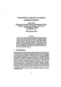
In any CSP instance some of the required relationships between variables are given explicitly in the constraints, whilst others generally arise implicitly from interactions among different constraints. For any instance in CSP(Γ), the explicit constraint relations must be elements of Γ, but there may be implicit restrictions on some subsets of the variables for which the corresponding relations are not elements of Γ, as the next example indicates. 4.1 Example Let Γ be the set containing a single binary relation, χ, over the set {0, 1, 2}, where χ is defined as follows: χ = {(0, 0), (0, 1), (1, 0), (1, 2), (2, 1), (2, 2)}. One element of CSP(Γ) is the instance P = ({v1 , v2 , v3 , v4 }, {0, 1, 2}, {C1 , C2 , C3 , C4 , C5 }), where C1 = ((v1 , v2 ), χ), C2 = ((v1 , v3 ), χ), C3 = ((v2 , v3 ), χ), C4 = ((v2 , v4 ), χ), C5 = ((v3 , v4 ), χ).

Figure 1: The CSP instance P defined in Example 4.1. Note that there is no explicit constraint on the pair (v1 , v4 ). However, by considering all solutions to P, it can be shown that the possible pairs of values which can be taken by this pair of variables are precisely the elements of the relation χ′ = χ ∪ {(1, 1)}. We now define exactly what it means to say that a constraint relation can be expressed in a constraint language.

190


4.2 Definition A relation ̺ can be expressed in a constraint language Γ over D if there exists a problem instance (V, D, C) in CSP(Γ), and a list, s, of variables, such that the solutions to (V, D, C) restricted to s give precisely the tuples of ̺. For any constraint language Γ, the set of all relations which can be expressed in Γ will be called the expressive power of Γ. The expressive power of a constraint language Γ can be characterised in a number of different ways [45]. For example, it is equal to the set of all relations that may be obtained from the relations in Γ using the relational join and project operations from relational database theory [37]. Alternatively, it can be shown to be equal to the set of relations definable by primitive positive formulas involving the relations of Γ and equality, which is defined as follows. 4.3 Definition For any set of relations Γ over D, the set "Γ# consists of all relations that can be expressed using (1) relations from Γ, together with the binary equality relation on D (denoted =D ), (2) conjunction, and (3) existential quantification. 4.4 Example Example 4.1 demonstrates that the relation χ′ belongs to the expressive power of the constraint language Γ = {χ}. It is easy to deduce from the construction given in Example 4.1 that χ′ (x, y) ≡ ∃ u ∃ v (χ(x, u) ∧ χ(x, v) ∧ χ(u, v) ∧ χ(u, y) ∧ χ(v, y)). Hence, χ′ ∈ "{χ}#.

4.2

Polymorphisms and complexity

In this section we shall explore how the notion of expressive power may be used to simplify the analysis of the complexity of the constraint satisfaction problem. We first note that any relation that can be expressed in a language Γ can be added to Γ without changing the complexity of CSP(Γ). 4.5 Proposition For any constraint language Γ and any relation ̺ belonging to the expressive power of Γ, CSP(Γ ∪ {̺}) is reducible in polynomial time to CSP(Γ). This result can be established simply by noting that, given an arbitrary problem instance in CSP(Γ∪{̺}), we can obtain an equivalent instance in CSP(Γ) by replacing each constraint C that has constraint relation ̺ with a collection of constraints that have constraint relations chosen from Γ and that together express the constraint C. By iterating this procedure we can obtain the following corollary. 4.6 Corollary For any constraint language Γ, and any finite constraint language Γ0 , if Γ0 is contained in the expressive power of Γ, then CSP(Γ0 ) is reducible to CSP(Γ) in polynomial time.

191


Corollary 4.6 implies that for any finite constraint language Γ, the complexity of CSP(Γ) is determined, up to polynomial-time reduction, by the expressive power of Γ, and hence by "Γ#. This raises an obvious question: how can we obtain sufficient information about the set "Γ# to determine the complexity of CSP(Γ)? A very successful approach to this question has been developed in [16, 42, 44], using techniques from universal algebra [62, 70]. To describe this approach, we need to consider (n) finitary operations on D. We will use OD to denote the set of all n-ary operations on the (n) set D (that is, the set of mappings f : D n → D), and OD to denote the set ∞ n=1 OD . (n) An operation f ∈ OD will be called essentially unary if there exists some i in the range (1) 1 ≤ i ≤ n, and some operation g ∈ OD such that the following identity is satisfied f (x1 , x2 , . . . , xn ) = g(xi ). An essentially unary operation for which g is the identity operation is called a projection. Any operation (of whatever arity) which is not essentially unary will be called essentially non-unary. Any operation on D can be extended in a standard way to an operation on tuples over (n) D, as follows. For any operation f ∈ OD , and any collection of tuples ?a1 ,?a2 , . . . ,?an ∈ Dm , where ?ai = (ai1 , . . . , aim ) (i = 1 . . . n), define f (?a1 , . . . ,?an ) by setting f (?a1 , . . . ,?an ) = (f (a11 , . . . , an1 ), . . . , f (a1m , . . . , anm )). (m)

(n)

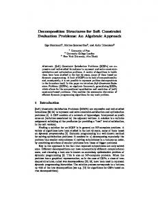
4.7 Definition For any relation ̺ ∈ RD , and any operation f ∈ OD , if f (?a1 , . . . ,?an ) ∈ ̺ for all choices of ?a1 , . . . ,?an ∈ ̺, then ̺ is said to be invariant under f , and f is called a polymorphism of ̺. The set of all relations that are invariant under each operation from some set C ⊆ OD will be denoted Inv(C). The set of all operations that are polymorphisms of every relation from some set Γ ⊆ RD will be denoted Pol(Γ). The operators Inv and Pol form a Galois correspondence between RD and OD (see [70, Proposition 1.1.14]). A basic introduction to this correspondence can be found in [68], and a comprehensive study in [70]. Sets of operations of the form Pol(Γ) are known as clones and sets of relations of the form Inv(C) are known as relational clones [70]. Moreover, the following useful characterisation of sets of the form Inv(Pol(Γ)) can be found in [70]. 4.8 Theorem For every set Γ ⊆ RD , Inv(Pol(Γ)) = "Γ#. This result was combined with Corollary 4.6 to obtain the following result in [42]. 4.9 Theorem For any constraint languages Γ, Γ0 ⊆ RD , with Γ0 finite, if Pol(Γ) ⊆ Pol(Γ0 ), then CSP(Γ0 ) is reducible to CSP(Γ) in polynomial time. This result implies that, for any finite constraint language Γ over a finite set, the complexity of CSP(Γ) is determined, up to polynomial-time reduction, by the polymorphisms of Γ. We now apply this result to obtain a sufficient condition for NP-completeness of CSP(Γ). A constraint language Γ is said to be strongly rigid if Pol(Γ) consists of projections only.

192


Figure 2: The operators Inv and Pol. 4.10 Proposition If Γ is strongly rigid then CSP(Γ) is NP-complete. This proposition follows from Theorem 4.9 by setting Γ0 = {N } (see Example 3.4), assuming {0, 1} ⊆ D, and using the fact that every relation on D is invariant under any projection. Proposition 4.10 was used in [58] to show that most non-trivial problems of the form CSP(Γ), with finite Γ, are NP-complete. More precisely, let R(n, k) denote a random kary relation on the set {1, . . . , n}, for which the probability that (a1 , . . . , ak ) ∈ R(n, k) is equal to 1/2 independently for each k-tuple (a1 , . . . , ak ) where not all ai ’s are equal; also, set (a, . . . , a) ∈ R(n, k) for all a (this is necessary to ensure that CSP(R(n, k)) is non-trivial). It is shown in [58] that the probability that {R(n, k)} is strongly rigid tends to 1 as either n or k tends to infinity.

4.3

Complexity of Boolean problems

In this section we describe some of the results that have been obtained concerning the complexity of Boolean constraint problems, that is, problems over a two-valued domain. The first result of this kind was a complete classification of the complexity of the ordinary Boolean constraint satisfaction problem obtained by Schaefer in 1978 [74]. Recall that a computational problem is called tractable if there is a polynomial-time algorithm deciding every instance of the problem. The class of all tractable problems is denoted PTIME. 4.11 Theorem For any constraint language Γ ⊆ R{0,1} , CSP(Γ) is tractable when (at least) one of the following conditions holds: (1) Every ̺ in Γ contains the tuple (0, 0, . . . , 0). (2) Every ̺ in Γ contains the tuple (1, 1, . . . , 1).


193

(3) Every ̺ in Γ is definable by a CNF formula in which each conjunct has at most one negated variable. (4) Every ̺ in Γ is definable by a CNF formula in which each conjunct has at most one unnegated variable. (5) Every ̺ in Γ is definable by a CNF formula in which each conjunct has at most two literals. (6) Every ̺ in Γ is definable by a system of linear equations over the two-element field. In all other cases CSP(Γ) is NP-complete. This result establishes a dichotomy for versions of this problem parameterized by the choice of constraint language: they are all either tractable or NP-complete. Dichotomy theorems of this kind are of particular interest because, on the one hand, they determine the precise complexity of particular constraint problems, and, on the other hand, they demonstrate that no problems of intermediate complexity can occur in this context. Note that the existence of constraint problems of intermediate complexity cannot be ruled out a priori due to the result [56] that if PTIME = NP then the class NP contains (infinitely many pairwise inequivalent) problems which are neither tractable nor NP-complete. Using the algebraic approach described in the previous sections, together with the knowledge of possible clones on a two-element set obtained in [71], Schaefer’s result can be reformulated in the following much more concise form. 4.12 Theorem For any set of relations Γ ⊆ R{0,1} , CSP(Γ) is tractable when Pol(Γ) contains any essentially non-unary operation or a constant operation. Otherwise it is NP-complete. 4.13 Example Recall the relation N over {0, 1} defined in Example 3.4. Using general results from [71], it can be shown that Pol({N }) contains essentially unary operations only, and hence, by Theorem 4.12, CSP({N }) is NP-complete. Schaefer’s result has inspired a series of analogous investigations for many related constraint problems, including those listed in Section 2. We will now list some complexity classification results that have recently been obtained for these problems in the Boolean case. Surprisingly, for a wide variety of such related problems it turns out that the polymorphisms of the constraint language are highly relevant to the study of the computational complexity. 4.14 Theorem Let Γ ⊆ R{0,1} be a Boolean constraint language. The following facts are known to hold for constraint problems parameterized by Γ: • The Counting Problem is tractable if Pol(Γ) contains the unique affine operation on {0, 1}, x − y + z. Otherwise it is #P-complete [20]. • The Quantified Problem is tractable if Pol(Γ) contains an essentially non-unary operation. Otherwise it is PSPACE-complete [20, 22]. • The Equivalence problem is tractable if Pol(Γ) contains an essentially non-unary operation or a constant operation. Otherwise it is coNP-complete [6].

194

A. Krokhin, A. Bulatov, and P. Jeavons • The Inverse Satisfiability problem is tractable if Pol(Γ) contains an essentially nonunary operation. Otherwise it is coNP-complete [49]. • The Maximum Hamming Distance problem is tractable if Pol(Γ) contains either a constant operation, or the affine operation and the negation operation on {0, 1} [21].

A full description of these results requires the careful definition of the relevant complexity classes and reductions, which is beyond the scope of this paper, so we refer the reader to the cited papers for details. 4.15 Example Recall the relation N over {0, 1} defined in Example 3.4. Using general results from [71], it can be shown that Pol({N }) contains essentially unary operations only. Hence, by Theorem 4.14, we can immediately conclude that: • Counting the number of solutions to an instance of CSP({N }) is #P-complete; • Deciding whether a quantified Boolean formula, whose quantifier-free part involves only conjunctions of the predicate N , is true is PSPACE-complete. • Deciding whether two instances of CSP({N }) have the same solutions is coNP-complete; • Deciding whether a given set of n-tuples is the set of solutions to some instance of CSP({N }) is coNP-complete.

4.4

From the CSP to algebras and varieties

Most of the results presented in this section were first obtained in [14, 17, 16]. With any constraint language Γ ⊆ RD one can associate an algebra AΓ = (D; Pol(Γ)). In this section we show that the complexity of the problem CSP(Γ) is completely determined by certain properties of AΓ . (We refer the reader to [62] for a general background in universal algebra.) Recall that algebras are said to be term equivalent if they have the same set of term operations. Since, the term operations of AΓ are precisely the operations in Pol(Γ), Theorem 4.9 implies that term equivalent algebras give rise to problem classes of the same complexity. 4.16 Proposition Let Γ1 , Γ2 ⊆ RD , where D is finite. If AΓ1 and AΓ2 are term equivalent then Γ1 and Γ2 are tractable or NP-complete simultaneously. This allows us to introduce the notion of a tractable algebra. 4.17 Definition An algebra A = (D; F ) is said to be tractable if the constraint language Inv(F ) is tractable. It is said to be NP-complete if Inv(F ) is NP-complete. Thus, the complexity classification problem for constraint languages reduces to the complexity classification problem for finite algebras. Furthermore, the next results show that it is possible to significantly restrict the class of algebras which need to be classified. Let A = (D; F ) be an algebra, and U ⊆ D. Let A|U denote the algebra A|U = (U, F ′ ), where F ′ consists of all operations of the form f |U (the restriction of f to U ), for each term operation f of A such that f ∈ Pol(U ).


195

4.18 Proposition Let A be a finite algebra, f a unary term operation such that f (f (x)) = f (x) and U = f (D). Then A is tractable if and only if A|U is tractable. Hence, by choosing a unary term operation with a minimal range, we may restrict ourselves to considering only surjective algebras, that is, algebras all of whose term operations are surjective. Recall that an operation f is called idempotent if it satisfies the identity f (x, . . . , x) = x, and the full idempotent reduct of an algebra A = (D; F ) is the algebra Id(A) = (D, F ′ ) where F ′ consists of all idempotent term operations of A. 4.19 Proposition A surjective finite algebra A is tractable if and only if its full idempotent reduct is tractable. It follows that to classify the complexity of arbitrary finite algebras it is sufficient to consider only idempotent algebras, that is, algebras whose operations are all idempotent. Next, we show that the standard algebraic constructions preserve the tractability of an algebra. 4.20 Theorem Let A be a finite algebra. If A is tractable, then all of its subalgebras, homomorphic images and finite direct powers are also tractable. Conversely, if A has an NPcomplete subalgebra, homomorphic image, or finite direct power, then it is NP-complete itself. For an algebra A, we denote the pseudo-variety and the variety generated by A by pvar(A) and var(A), respectively. 4.21 Corollary A finite algebra A is tractable if and only if every algebra from pvar(A) is tractable. As is well known, if A is a finite class of finite algebras, then the pseudo-variety generated by A equals the class of finite algebras from the variety generated by A. 4.22 Corollary A finite algebra A is tractable if and only if every finite algebra from var(A) is tractable. 4.23 Corollary If A is a finite algebra, and var(A) contains a finite NP-complete algebra, then A is NP-complete. Thus, the tractability of an algebra is a property which can be determined by identities. We call an algebra a set if it contains more than one element and all of its operations are projections. By combining Proposition 4.10 with Corollary 4.23, we get the following result. 4.24 Corollary If the pseudovariety generated by a finite idempotent algebra A contains a set then A is NP-complete. A homomorphic image of a subalgebra of an algebra A is called a factor of A. 4.25 Proposition If A is an idempotent algebra and pvar(A) contains a set then some factor of A is a set.

196


Remarkably, the presence of a set as a factor is the only known reason for an idempotent algebra to be NP-complete. This prompts us to suggest the following conjecture. 4.26 Conjecture A finite idempotent algebra A is tractable if and only if none of the factors of A is a set;

(No-Set)

otherwise it is NP-complete. It was shown in [17] that if one strengthens Conjecture 4.26 by removing the condition of idempotency, or replacing “factor” by either “subalgebra” or “homomorphic image”, then the resulting conjecture is false. It was proved in [78] that a variety V generated by a finite idempotent algebra contains no set if and only if there is an n-ary term f (called a Taylor term) in V such that V satisfies n identities of the form f (xi1 , . . . , xin ) = f (yi1 , . . . , yin ),

i = 1, . . . , n,

where xij , yij ∈ {x, y} and xii = yii for all i, j. Therefore, Corollary 4.24 can be restated as follows. 4.27 Corollary If a finite idempotent algebra has no Taylor term, then it is NP-complete. This corollary was used in [57] to study systems of polynomial equations over finite algebras, where it was proved, in particular, that solving systems of equations over a non-trivial algebra from a congruence-distributive variety is NP-complete, and, furthermore, solving systems of equations over a Mal’tsev algebra is tractable if this algebra is polynomially equivalent to a module, otherwise it is NP-complete. Using the result from [78] mentioned above, Conjecture 4.26 can be restated in terms of identities. 4.28 Conjecture A finite idempotent algebra A is tractable if it has a Taylor term; otherwise it is NP-complete. Finally, the condition (No-Set) from Conjecture 4.26 can be expressed in terms of tame congruence theory [40]: a finite idempotent algebra satisfies this condition if and only if the variety it generates “omits type 1” [14].

4.5 4.5.1

Tractable algebras, classification results and tractability tests Tractable algebras

During the last decade several particular identities (particular forms of the Taylor term) have been identified that guarantee the tractability of algebras satisfying one of these identities (that is, having a Taylor term of one of these special forms) [12, 10, 26, 42, 43, 44]. Recall that a binary operation · is called a 2-semilattice operation if it satisfies the identities x · x = x, x · y = y · x and (x · x) · y = x · (x · y). Note that a semilattice operation is a particular case of a 2-semilattice operation. A ternary operation f satisfying the identities


197

f (x, y, y) = f (y, y, x) = x is called a Mal’tsev operation, and an n-ary operation g is called a near-unanimity operation if it satisfies the identities f (y, x, . . . , x) = f (x, y, x, . . . , x) = · · · = f (x, . . . , x, y) = x. An n-ary operation is called totally symmetric if, for all x1 , . . . , xn and y1 , . . . , yn such that {x1 , . . . , xn } = {y1 , . . . , yn }, it satisfies the identities f (x1 , . . . , xn ) = f (y1 , . . . , yn ). (Note that, in [26], a family (fn )n≥2 of totally symmetric operations, where fn is n-ary, was called a set function). 4.29 Theorem [12, 10, 43, 26] A finite algebra is tractable if it has (at least) one the following: • a 2-semilattice term operation; • a Mal’tsev term operation; • a near-unanimity term operation; • n-ary totally symmetric term operations for all n ≥ 2. Another class of algebras which has been shown to be tractable [24] is the class of paraprimal algebras, which are defined as follows. Let ̺ an n-ary relation on D, and I = {i1 , . . . , ik } ⊆ {1, . . . , n} with i1 < · · · < ik . By the projection of ̺ onto I we mean the relation ̺|I = {(ai1 , . . . , aik ) | (a1 , . . . , an ) ∈ ̺}. The set I is said to be ̺-reduced if it is minimal with the property that the natural mapping ̺ → ̺|I is one-to-one. A finite algebra A is called para-primalif, for every n ∈ N, every subuniverse ̺ of An , and every ̺-reduced set I, we have ̺|I = i∈I ̺|{i} . However, it is known that every para-primal algebra has a Mal’tsev term operation (see [76, Theorem 4.7]), and, hence, tractability of para-primal algebras follows from Theorem 4.29. 4.5.2

Classification results

Algebras of several special types have been completely classified with respect to the complexity of the corresponding constraint satisfaction problems. Strictly simple algebras A finite algebra is said to be strictly simple if it is simple and has no subalgebras with more than one element. Strictly simple algebras are completely described in [77]. 4.30 Proposition [17, 16] A finite idempotent strictly simple algebra is tractable if it is not a set; otherwise it is NP-complete. Homogeneous algebras An algebra is called homogeneous if every permutation on its base set is an automorphism of the algebra. Finite homogeneous algebras are completely described in [60]. 4.31 Proposition [24] A finite homogeneous algebra is tractable if it satisfies the condition ( No-Set); otherwise it is NP-complete.

198


Finite semigroups A semigroup is called a left- [right-]zero semigroup if x·y = x [x·y = y] for all x, y. It is called a block-group if none of its subsemigroups is a left- or right-zero semigroup. As is easily seen, block-groups are exactly those semigroups that have no factor which is a set. 4.32 Proposition [15] A finite semigroup is tractable if it is a block-group; otherwise it is NP-complete. Small algebras

Conjecture 4.26 has been proved for 2- and 3-element algebras.

4.33 Theorem [74, 9] (1) An idempotent two-element algebra is tractable if it is not a set; otherwise it is NPcomplete. (2) An idempotent three-element algebra is tractable if it satisfies the condition (No-Set); otherwise it is NP-complete. Conservative algebras An algebra is said to be conservative if every subset of its universe is a subalgebra, or, equivalently, if f (x1 , . . . , xn ) ∈ {x1 , . . . , xn } for every term operation f and all x1 , . . . , xn . 4.34 Theorem [11] A conservative algebra A is tractable if every 2-element subalgebra B has a term operation of one of the following types: a semilattice operation, a ternary nearunanimity operation (that is, a majority operation), or a Mal’tsev operation; otherwise A is NP-complete. It is not hard to check that the conditions stated in Theorem 4.34 are equivalent to (No-Set). 4.5.3

Testing tractability

We now consider the problem of deciding whether a given constraint language or idempotent algebra is tractable. Following [20], we call such a problem a meta-problem. A priori, there is no upper complexity bound for this problem; it may even be undecidable. However, if Conjecture 4.26 is true, then, given the basic operations of an idempotent algebra, one can straightforwardly check whether any factor of the algebra is a set. If we are given a finite constraint language Γ on a finite set A, then the presence of a factor which is a set can be detected by examining all polymorphisms of Γ of arity at most |A|. Thus, the meta-problem is decidable, assuming Conjecture 4.26 holds. In this section we study its complexity. For a constraint language Γ, let f ∈ Pol(Γ) be a unary operation with minimal range U , and let f (Γ) = {f (̺) | ̺ ∈ Γ} where f (̺) = {f (?a) | ?a ∈ ̺}. Denote by Γ the constraint language f (Γ) ∪ {{a} | a ∈ U }. It follows from Propositions 4.18 and 4.19 that Γ is tractable if and only if Γ is tractable. Moreover, the algebra AΓ = (U, Pol(Γ) is idempotent. We consider three combinatorial decision problems related to the condition (No-Set). CSP-Tractability-of-algebra Instance: A finite set A and operation tables of idempotent operations f1 , . . . , fn on A. Question: Does the algebra A = (A; {f1 , . . . , fn }) satisfy (No-set)?


199

CSP-Tractability Instance: A finite set A and a finite constraint language Γ on A. Question: Does the algebra A = (U, Pol(Γ)) satisfy (No-set)? CSP-Tractability(k) Instance: A finite set A, |A| ≤ k, and a finite constraint language Γ on A. Question: Does the algebra A = (U, Pol(Γ)) satisfy (No-set)? 4.35 Theorem [14] (1) The problem CSP-Tractability-of-algebra is tractable. (2) The problem CSP-Tractability(k) is tractable. (3) The problem CSP-Tractability is NP-complete. The algorithm solving CSP-Tractability-of-algebra is, in fact, an adapted version of the algorithm presented in [3] for finding the type set of a finite algebra. Since this algorithm uses operations of arity bounded by the size of the algebra, it can be further transformed to an algorithm for solving CSP-Tractability(k). Finally, it is possible to show that CSP-Tractability is in NP and to reduce the NP-complete problem Not-All-EqualSatisfiability (see Example 3.4) to CSP-Tractability in polynomial time.

4.6

The counting CSP

In this section we discuss Problem 3.6 for the counting constraint satisfaction problem (#CSP), which is the problem of counting solutions to an instance of CSP. Using the logical and the homomorphism forms of the CSP (see Section 1) this problem can also be formulated as the problem of counting satisfying assignments to a conjunctive formula, that is, a formula of the form ̺1 ∧ · · · ∧ ̺n , where each ̺i is an atomic formula, in a given interpretation, or alternatively as the problem of finding the number of homomorphisms between two finite relational structures. For any constraint language Γ, giving rise to the decision constraint satisfaction problem CSP(Γ), we also define the corresponding class #CSP(Γ) of counting problems. The results of this section were first obtained in [13]. 4.36 Example An instance of the #3-SAT problem [19, 20, 80, 81] is specified by giving an instance of the 3-satisfiability problem (see Example 1.3) and asking how many assignments satisfy it. Therefore, #3-SAT is equivalent to #CSP(Γ) where Γ is the set of ternary Boolean relations which are expressible by clauses. 4.37 Example In the problem Antichain [72], we are given a finite poset (P ; ≤), and we aim to compute the number of antichains in P . This problem can be expressed in the #CSPform as follows. Let ̺≤ be the predicate of the natural order on {0, 1}. ! We assign a variable xa to each element a ∈ P . Then the #CSP({̺≤ }) instance Φ = a≤b ̺≤ (xa , xb ) can be shown to be equivalent to the original Antichain instance.

200


To show this, notice that every model ϕ to Φ satisfies the following condition: if ϕ(xa ) = 1 and a ≤ b then ϕ(xb ) = 1. This means that the set Fϕ = {a ∈ P | ϕ(xa ) = 1} is a filter of P . Hence the models of Φ correspond one-to-one to the filters of P , and consequently, to the antichains of P . On the other hand, any #CSP({̺≤ }) instance is reducible to an Antichain instance, though not so straightforwardly (see [13]). Thus Antichain is equivalent to #CSP({̺≤ }). The general #CSP is known to be #P-complete, as follows from Theorem 4.14, or the results of [81] and the examples above. We call a constraint language Γ #-tractable if, for every finite Γ0 ⊆ Γ, the problem #CSP(Γ0 ) is polynomial time solvable. The language Γ is said to be #P-complete if #CSP(Γ0 ) is #P-complete for a certain finite Γ0 ⊆ Γ. The expressive power and the polymorphisms of a constraint language again play crucial roles in determining the complexity of #CSP(Γ). 4.38 Proposition For any constraint languages, Γ, Γ0 , on a finite set D, with Γ0 finite, if Γ0 ⊆ "Γ#, then #CSP(Γ0 ) is reducible to #CSP(Γ) in polynomial time. 4.39 Proposition For any constraint languages Γ, Γ0 , on a finite set D, with Γ0 finite, if Pol(Γ) ⊆ Pol(Γ0 ), then #CSP(Γ0 ) is reducible to #CSP(Γ) in polynomial time. Proposition 4.39 implies that, as with the decision CSP, the algebra AΓ fully determines the counting complexity of a constraint language Γ. We will say that a finite algebra A = (D; F ) is #-tractable [#P-complete] if so is the constraint language Inv(F ). The next result shows that, once again, standard constructions preserve tractability. 4.40 Theorem Let A be a finite algebra. If A is #-tractable, then all of its subalgebras, homomorphic images and finite direct powers are also #-tractable. Conversely, if A has a #P-complete subalgebra, homomorphic image, or finite direct power, then A is #P-complete itself. 4.41 Theorem A finite algebra is #-tractable (#P-complete) if and only if its full idempotent reduct is #-tractable (#P-complete). The benchmark hard counting problems arise from binary reflexive non-symmetric relations. 4.42 Proposition If ̺ is a binary reflexive non-symmetric relation on a finite set, then #CSP({̺}) is #P-complete. Theorem 4.40, Proposition 4.42, and the results from [40], provide a link between the complexity of #CSP and Mal’tsev operations, which we will now investigate. The next statement follows from [40, Theorem 9.13]. 4.43 Theorem For a finite algebra A the following conditions are equivalent: (1) A does not have a Mal’tsev term operation. (2) There is a finite algebra B = (B; F ) ∈ var(A), such that Inv(F ) contains a binary reflexive non-symmetric relation.


201

By Proposition 4.42, the algebra B from Theorem 4.43 (2) is #P-complete. Furthermore, Theorem 4.40 implies that A is also #P-complete. 4.44 Corollary Every finite algebra having no Mal’tsev term operation is #P-complete. By making use of Corollary 4.44 we can obtain a very easy proof of the dichotomy theorem for the Boolean #CSP ([19], see Theorem 4.14). First, it follows from the results of [71], that any Boolean relation which is invariant under some Mal’tsev operation on {0, 1} is also invariant under the unique affine operation on {0, 1}, x − y + z. Hence, by Corollary 4.44, any Boolean constraint language is either #P-complete, or else a subset of Inv({x − y + z}). Any relation belonging to Inv({x − y + z}) is the solution space of a system of linear equations over the 2-element field, so it is possible to find a basis for this set in polynomial time. Furthermore, the number of solutions in this set equals 2n , where n is the number of vectors in the basis. 4.45 Example The #H-coloring problem is the counting version of the Graph Hcoloring problem (see Example 3.5). In this problem, the goal is to find the number of homomorphisms from a given graph G to the fixed graph H. If the #H-coloring problem is restricted to undirected graphs then, as proved in [28], the problem is tractable if every connected component of H is either an isolated vertex, or a complete graph with all loops, or a complete unlooped bipartite graph; otherwise the problem is #P-complete. The tractability part of this result is easy, and the hardness part can be easily derived from Corollary 4.44, since symmetric relations (or graphs) invariant under a Mal’tsev operation must be of the form specified above. We will now describe a sufficient condition for Mal’tsev algebras to be #-tractable. An algebra is said to be uniform if, for any subalgebra B, the blocks of every congruence of B are of the same size. Clearly, all two-element algebras, groups and quasi-groups are uniform. 4.46 Theorem Every uniform Mal’tsev algebra is #-tractable.

4.7

The Quantified CSP

The standard constraint satisfaction problem over an arbitrary finite domain can be expressed as follows: given a first-order sentence of the form ∃ x1 . . . ∃ xl (̺1 ∧ . . . ̺q ), where each ̺i is an atomic formula, and x1 , . . . , xl are the variables appearing in the ̺i , determine whether the sentence is true (see Section 1). In this subsection we consider a more general framework which allows arbitrary quantifiers over constrained variables, rather than just existential quantifiers. This form of the CSP is called the quantified CSP, or QCSP for short. The Boolean QCSP (also known as QSAT or QBF), and some of its restrictions (such as Q3SAT), have always been standard examples of PSPACE-complete problems [32, 66, 74]. All the results presented in this section were first obtained in [8, 18]. 4.47 Definition For a constraint language Γ ⊆ RD , an instance of QCSP(Γ) is a firstorder sentence Q1 x1 . . . Ql xl (̺1 ∧ · · · ∧ ̺q ), where each ̺i is an atomic formula involving a predicate from Γ, x1 , . . . , xl are the variables appearing in the ̺i , and Q1 , . . . , Ql are arbitrary quantifiers. The question is whether the sentence is true.

202


Clearly, an instance of CSP(Γ) corresponds to an instance of QCSP(Γ) in which all the quantifiers happen to be existential. We note that in the Boolean case, the complexity of QCSP(Γ) has been completely classified (see Theorem 4.11). For problems over larger domains no complete classification has yet been obtained, but there are a number of known results concerning the complexity of special cases. 4.48 Example Consider the following Coloring Construction Game played by two players, Player 1 and Player 2: given an undirected graph G = (V, E), a linear ordering on V (i.e., a bijection f : V → {1, . . . , |V |}), an ownership function w : V → {1, 2} (that is, each vertex v is “owned” by Player w(v)), and a finite set of colours D with |D| ≥ 3. In the i’th move, the player who owns vertex f −1 (i) (that is, Player w(f −1 (i))) colours it in one of |D| available colours. Player 1 wins if all vertices are coloured at the end of the game. Deciding whether Player 1 has a winning strategy in an instance of this game can be translated into an instance of the quantified version of the Graph |D|-colorability problem, QCSP({=D }). To make this translation we view elements from V as variables, elements of E as constraint scopes, the relation =D as the only available constraint relation, the variables from w−1 (1) as existentially quantified, the variables from w−1 (2) as universally quantified, and the order of quantification as specified by the function f . The problem QCSP({=D }) was shown to be PSPACE-complete [8]. It can be shown that, for quantified constraint satisfaction problems, surjective polymorphisms play a similar role to that played by arbitrary polymorphisms for ordinary CSPs (cf. Theorem 4.9). Let s-Pol(Γ) denote the set of all surjective operations from Pol(Γ). 4.49 Theorem For any constraint languages Γ, Γ0 ⊆ RD , with Γ0 finite, if s-Pol(Γ) ⊆ s-Pol(Γ0 ), then QCSP(Γ0 ) is reducible to QCSP(Γ) in polynomial time. This theorem follows immediately from the next two propositions. 4.50 Definition For any set Γ ⊆ RD , the set [Γ] consists of all predicates that can be expressed using: (1) predicates from Γ, together with the binary equality predicate =D on D, (2) conjunction, (3) existential quantification, (4) universal quantification. 4.51 Proposition For any constraint languages Γ, Γ0 ⊆ RD , with Γ0 finite, if [Γ0 ] ⊆ [Γ], then QCSP(Γ0 ) is reducible to QCSP(Γ) in polynomial time. 4.52 Proposition For any constraint language Γ over a finite set, [Γ] = Inv(s-Pol(Γ)). Note that Proposition 4.52 intuitively means that the expressive power of constraints in the QCSP is determined by their surjective polymorphisms. Hence, in order to show that some relation ̺ belongs to [Γ], one does not have give an explicit construction, but instead one can show that ̺ is invariant under all surjective polymorphisms of Γ, which often turns out to be significantly easier.

203


We remark that the operators Inv() and s-Pol() used in Proposition 4.52 form a Galois connection between RD and the set of all surjective members of OD which has not previously been investigated (see, e.g., survey [69]). Using Theorem 4.49, together with Example 4.48, we can obtain a sufficient condition for PSPACE-completeness of QCSP(Γ), in terms of the surjective polymorphisms of Γ. 4.53 Theorem For any finite set D with |D| ≥ 3, and any Γ ⊆ RD , if every f ∈ s-Pol(Γ) is of the form f (x1 , . . . , xn ) = g(xi ) for some 1 ≤ i ≤ n and some permutation g on D, then QCSP(Γ) is PSPACE-complete. The next example uses this result to show that even predicates that give rise to trivial constraint satisfaction problems can give rise to intractable quantified constraint satisfaction problems. This can happen because non-surjective polymorphisms, which may guarantee the tractability of the CSP, do not affect the complexity of the QCSP. 4.54 Example Let τs be the s-ary “not-all-distinct” predicate holding on a tuple (a1 , . . . , as ) if and only if |{a1 , . . . , as }| < s. Note that τs ⊇ {(a, . . . , a) | a ∈ D}, so every instance of CSP({τs }) is trivially satisfiable by assigning the same value to all variables. However, by [70, Lemma 2.2.4], the set Pol({τ|D| }) consists of all non-surjective operations on D, together with all operations of the form given in Theorem 4.53. Hence, {τ|D| } satisfies the conditions of Theorem 4.53, and QCSP({τ|D| }) is PSPACE-complete. Similar arguments can be used to show that QCSP({τs }) is PSPACE-complete, for any s in the range 3 ≤ s ≤ |D|. On the tractability side, we have the following result. We call a semilattice operation bounded if the corresponding partial order is bounded (that is, it is a lattice order). Recall that the dual discriminator operation is defined by the rule " y d(x, y, z) = x

if y = z, otherwise.

Note that the dual discriminator is a special type of near-unanimity operation. 4.55 Theorem For any constraint language Γ over a finite set: (1) if Pol(Γ) contains a Mal’tsev operation, or a near-unanimity operation, or a bounded semilattice operation, then QCSP(Γ) is tractable; (2) if Pol(Γ) contains the dual discriminator operation, then QCSP(Γ) is in NL. Recall that the graph of a permutation π is the binary relation {(x, y) | y = π(x)} (or the binary predicate π(x) = y), For the special case when Γ contains the set ∆ of all graphs of permutations, there is a trichotomy result which says that such problems are either tractable, or NP-complete, or PSPACE-complete. (We remark that the complexity of the standard CSP(Γ) for such sets Γ was completely classified in [24].) To state this trichotomy result we need to define two additional surjective operations:

204

A. Krokhin, A. Bulatov, and P. Jeavons • The k-ary near projection operation, " x1 lk (x1 , . . . , xk ) = xk

if x1 , . . . , xk are all different, otherwise.

• The ternary switching operation,   x s(x, y, z) = y   z

if y = z, if x = z, otherwise.

4.56 Theorem Let ∆ ⊆ Γ ⊆ RD , and |D| ≥ 3.

• If s-Pol(Γ) contains the dual discriminator d, or the switching operation s, or (when |D| ∈ {3, 4}) an affine operation, then QCSP(Γ) is in PTIME; • otherwise, if s-Pol(Γ) contains l|D| , then QCSP(Γ) is NP-complete; • otherwise QCSP(Γ) is PSPACE-complete.

5

The infinite-valued CSP

There are many computational problems which can be represented as constraint satisfaction problems, but require an infinite set of values. In order to avoid representation problems for infinite objects, we will consider CSPs with infinite sets of values in the following form: fix an infinite relational structure B of finite signature; the input then is a finite structure A of the same signature, and the question is whether there is a homomorphism from A to B. Here are two well-known examples of problems with an infinite set of possible values. 5.1 Example An instance of the Acyclic Digraph problem is a directed graph G, and the question is whether G is acyclic, that is, contains no directed cycles. It is easy to see that this problem is equivalent to Hom(B) where B = (N; f (b) > f (c). This problem is equivalent to Hom(B) with B = (N, R) where R = {(x, y, z) ∈ N3 | x < y < z or x > y > z}. This problem is NP-complete [32]. It was shown in Proposition 3.7 of [4] that the former problem cannot be represented as CSP(Γ) for any constraint language Γ over a finite set D (in fact, the above mentioned proposition is an even stronger claim); for the latter problem, the proof is similar.


5.1

205

Applicability of polymorphisms

For a family Γ of relations over an infinite set, let "Γ# be defined exactly as in the finite case (see Definition 4.3). In order to investigate the applicability of the algebraic approach, described in previous sections, to the infinite-valued CSP, the first question to be asked is whether the complexity is determined by the polymorphisms of the constraint relations; that is, whether "Γ# = Inv(Pol(Γ)) when Γ is a finite constraint language over an infinite domain. It is not hard to see that the inclusion "Γ# ⊆ Inv(Pol(Γ)) always holds. However, this inclusion can be strict, as the next example shows. 5.3 Example Consider Γ = {R1 , R2 , R3 } on N, where R1 = {(a, b, c, d) | a = b or c = d}, R2 = {(1)}, and R3 = {(a, a+ 1) | a ∈ N}. It is not difficult to show that every polymorphism of Γ is a projection, and hence Inv(Pol(Γ)) is the set of all relations on N. However, one can check that, for example, the unary relation consisting of all even numbers does not belong to "Γ#. However, for some countable structures B, the required equality does hold, as the next result indicates. A countable structure B (of finite signature) is called homogeneous if every isomorphism between any pair of substructures is induced by an automorphism of B. A countable structure is called ω-categorical if it is determined (up to isomorphism) by its first-order theory. It is known that every countable homogeneous structure is ω-categorical, and that a countable structure is ω-categorical if and only if its automorphism group, when acting on the set of all n-tuples (for any n) of elements from the structure, has only finitely many orbits (see, e.g., [41]). 5.4 Theorem [4, 5] If BΓ is a countable ω-categorical structure then "Γ# = Inv(Pol(Γ)). Many examples of countable homogeneous structures, as well as remarks on the complexity of the corresponding constraint satisfaction problems, can be found in [4, 5].

5.2

The interval-valued CSP

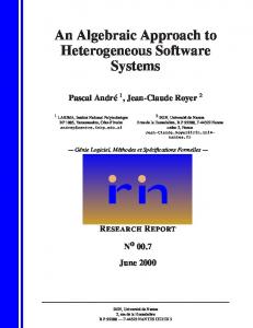
One form of infinite-valued CSP which has been widely studied in artificial intelliegence is the case where the values taken by the variables are intervals on the real line. This setting is used to model temporal behaviour of systems, where the intervals represent time intervals during which events occur. The most popular such formalism is Allen’s interval algebra (AIA for short), introduced in [1], which concerns binary qualitative relations between intervals. This algebra contains 13 basic relations (see Table 1), corresponding to the 13 distinct ways in which two given intervals can be related. The complete set of relations in AIA consists of the 213 = 8192 possible unions of the basic relations. Let Γ be a constraint language over the set of intervals on the real line, whose elements are members of Allen’s interval algebra, and let BΓ be the corresponding relational structure. It is not hard to see that every instance of CSP(Γ) can also be (more graphically) viewed as a directed graph whose vertices represent the variables and whose arcs are each labelled with a relation from Γ. The question would then be whether one can assign intervals to the vertices so that all constraints on the arcs are satisfied.

206


Table 1: The 13 basic relations in Allen’s interval algebra. Some well-known combinatorial problems can be represented as CSP(Γ) for a suitable subset Γ of AIA, as the next example indicates. 5.5 Example An undirected graph is called an interval graph if it possible to assign (open) intervals to its nodes so that two intervals intersect if and and only if the corresponding nodes are adjacent. An instance of the Interval Graph Sandwich problem [34] consists of two (undirected) graphs G1 = (V, E1 ) and G2 = (V, E2 ) such that E1 ⊆ E2 . The question is whether there is E such that E1 ⊆ E ⊆ E2 and G = (V, E) is an interval graph. This problem is known to be NP-complete [34]. This problem can be represented as CSP(Γ) where Γ consists of two relations: “disjoint” (given by p ∪ p−1 ∪ m ∪ m−1 ) and its complement, “intersect” (the union of the other nine basic relations). Indeed, let V be the set of variables; then, to any edge e ∈ E1 assign the constraint “intersect”, to any edge e ∈ E2 assign the constraint “disjoint”, and leave all other pairs of variables unrelated. Solutions of this CSP precisely correspond to interval graph sandwiches. Note that the case when G1 = G2 is known as Interval Graph Recognition problem, which is tractable, but this problem is not of the form CSP(Γ) because we cannot leave variables unrelated. Choosing other pairs of complementary relations, one can obtain other graph sandwich problems, such as the Overlap (or Circle) Graph Sandwich problem [34, 55] The general CSP problem for AIA is NP-complete, as follows from the above example. The problem of classifying subsets of AIA with respect to the complexity of the corresponding CSP has attracted much attention in artificial intelligence (see, for example, [75]). Allen’s interval algebra has three operations on relations: composition, intersection, and inversion. Note that these three operations can each be represented by using conjunction and existential quantification, so, for any subset Γ of AIA, the subalgebra Γ′ of AIA generated by Γ has the property that Γ′ ⊆ "Γ#. It follows from Lemma 3.3 of [4] (which is Corollary 4.6


207

Sp = {r | r ∩ (pmod−1 f −1 )±1 = ∅ ⇒ (p)±1 ⊆ r} Sd = {r | r ∩ (pmod−1 f −1 )±1 = ∅ ⇒ (d−1 )±1 ⊆ r} So = {r | r ∩ (pmod−1 f −1 )±1 = ∅ ⇒ (o)±1 ⊆ r} A1 = {r | r ∩ (pmod−1 f −1 )±1 = ∅ ⇒ (s−1 )±1 ⊆ r} A2 = {r | r ∩ (pmod−1 f −1 )±1 = ∅ ⇒ (s)±1 ⊆ r} A3 = {r | r ∩ (pmodf )±1 = ∅ ⇒ (s)±1 ⊆ r} A4 = {r | r ∩ (pmodf −1 )±1 = ∅ ⇒ (s)±1 ⊆ r} Ep = {r | r ∩ (pmods)±1 = ∅ ⇒ (p)±1 ⊆ r} Ed = {r | r ∩ (pmods)±1 = ∅ ⇒ (d)±1 ⊆ r} Eo = {r | r ∩ (pmods)±1 = ∅ ⇒ (o)±1 ⊆ r} B1 = {r | r ∩ (pmods)±1 = ∅ ⇒ (f −1 )±1 ⊆ r} B2 = {r | r ∩ (pmods)±1 = ∅ ⇒ (f )±1 ⊆ r} B3 = {r | r ∩ (pmod−1 s−1 )±1 = ∅ ⇒ (f −1 )±1 ⊆ r} B4 = {r | r ∩ (pmod−1 s)±1 = ∅ ⇒ (f −1 )±1 ⊆ r} E∗

S∗

' ( ) ( 1) r ∩ (pmod)±1 = ∅ ⇒ (s)±1 ⊆ r, and ( = r( 2) r ∩ (ff −1 ) = ∅ ⇒ (≡) ⊆ r

) ' ( ( 1) r ∩ (pmod−1 )±1 = ∅ ⇒ (f −1 )±1 ⊆ r, and = r (( 2) r ∩ (ss−1 ) = ∅ ⇒ (≡) ⊆ r

 (   (( 1) r ∩ (os)±1 = ∅ & r ∩ (o−1 f )±1 = ∅ ⇒ (d)±1 ⊆ r, and  H = r (( 2) r ∩ (ds)±1 = ∅ & r ∩ (d−1 f −1 )±1 = ∅ ⇒ (o)±1 ⊆ r, and  (  3) r ∩ (pm)±1 = ∅ & r ⊆ (pm)±1 ⇒ (o)±1 ⊆ r A≡ = {r | r = ∅ ⇒ (≡) ⊆ r}

Table 2: The 18 maximal tractable subalgebras of Allen’s algebra. for the infinite case) that CSP(Γ) and CSP(Γ′ ) are polynomial-time equivalent. Hence it is sufficient to classify all subalgebras of AIA. Using computations in subalgebras of AIA, manipulations with primitive positive formulas (called derivations in [55]) and a number of new NP-completeness results, a complete classification of the complexity of all subsets of AIA was accomplished in [55], where the following result was obtained. 5.6 Theorem Let Γ be a subset of Allen’s interval algebra. If Γ is contained in one of the eighteen subalgebras listed in Table 2, then CSP(Γ) is tractable; otherwise it is NP-complete. In Table 2, for the sake of brevity, relations between intervals are written as collections of basic relations. So, for instance, we write (pmod) instead of p ∪ m ∪ o ∪ d. We also use the symbol ±, which should be interpreted as follows: a condition involving ± means the conjunction of two conditions, one corresponding to + and one corresponding to −. For example, the condition (o)±1 ⊆ r ⇐⇒ (d)±1 ⊆ r means that both (o) ⊆ r ⇐⇒ (d) ⊆ r and (o−1 ) ⊆ r ⇐⇒ (d−1 ) ⊆ r hold.

208


It follows from Theorem 5.6 that CSP({r}), where r is a single relation in AIA, is NPcomplete if and only if r either satisfies r ∩ r −1 = (mm−1 ) or is a relation with r ∩ r −1 = ∅ and such that neither r nor r −1 is contained in one of (pmod−1 sf −1 ), (pmod−1 s−1 f −1 ), (pmodsf ) and (pmodsf −1 ). It was noted in [4, 5] that AIA (without its operations) is in fact a homogeneous relational structure. Since we may assume, without loss of generality, that all intervals under consideration have rational endpoints, we obtain a countable homogeneous structure of finite signature. Therefore, by Theorem 5.4, the complexity classification problem for subsets of AIA can be tackled using polymorphisms. Such an approach may provide a route to simplifying the involved classification proof given in [55].

References [1] J. F. Allen, Maintaining knowledge about temporal intervals, Comm. ACM 26 (1983), 832–843. [2] J. F. Allen, Natural Language Understanding, Benjamin Cummings, 1994. ´ Szendrei, The set of types of a finitely generated [3] J. Berman, E. Kiss, P. Pr¨ ohle, and A. variety, Discrete Math. 112 (1–3) (1993), 1–20. [4] M. Bodirsky, Constraint satisfaction with infinite domains, Ph.D. Thesis, Humboldt University, Berlin, 2004. [5] M. Bodirsky and J. Neˇsetˇril, Constraint satisfaction problems with countable homogeneous structures, in: Computer Science Logic (Vienna, 2003), Lecture Notes in Comput. Sci. 2803, Springer, Berlin, 2003, 44–57. [6] E. B¨ ohler, E. Hemaspaandra, S. Reith, and H. Vollmer, Equivalence and isomorphism for Boolean constraint satisfaction, in: Computer Science Logic (Edinburgh, 2002), Lecture Notes in Comput. Sci. 2471, Springer, Berlin, 2002, 412–426. [7] E. B¨ ohler, E. Hemaspaandra, S. Reith, and H. Vollmer, The complexity of Boolean constraint isomorphism, in: STACS 2004 (Montpellier, 2004), Lecture Notes in Comput. Sci. 2996, Springer, Berlin, 2004, 164–175. [8] F. B¨ orner, A. Bulatov, P. Jeavons, and A. Krokhin, Quantified constraints: Algorithms and complexity, in: Computer Science Logic (Vienna, 2003), Lecture Notes in Comput. Sci. 2803, Springer, Berlin, 2003, 58–70. [9] A. Bulatov, A dichotomy theorem for constraints on a three-element set, in: Foundations of Computer Science (Vancouver, BC, 2002), IEEE Comput. Soc., 2002, 649–658. [10] A. Bulatov, Mal’tsev constraints are tractable, Technical Report PRG-RR-02-05, Computing Laboratory, University of Oxford, UK, 2002. [11] A. Bulatov, Tractable conservative constraint satisfaction problems, in: Logic in Computer Science (Ottawa, ON, 2003), IEEE Comput. Soc., 2003, 321–330.


209

[12] A. Bulatov, Combinatorial problems raised from 2-semilattices, J. Algebra, accepted for publication. [13] A. Bulatov and V. Dalmau, Towards a dichotomy theorem for the counting constraint satisfaction problem, in: Foundations of Computer Science (Boston, MA, 2003), IEEE Comput. Soc., 2003, 562–571. [14] A. Bulatov and P. Jeavons, Algebraic structures in combinatorial problems, Technical Report MATH-AL-4-2001, Technische Universität Dresden, Germany, 2001. [15] A. Bulatov, P. Jeavons, and M. Volkov, Finite semigroups imposing tractable constraints, in: Semigroups, Algorithms, Automata and Languages (Gracinda M.S.Gomes, Jean-Eric Pin, Pedro V.Silva, eds), World Scientific, Singapore, 2002, 313–329. [16] A. Bulatov, A. Krokhin, and P. Jeavons, Constraint satisfaction problems and finite algebras, in: Automata, Languages and Programming (Geneva, 2000), Lecture Notes in Comput. Sci. 1853, Springer, Berlin, 2000, 272–282. [17] A. Bulatov, A. Krokhin, and P. Jeavons, Classifying complexity of constraints using finite algebras, SIAM J. Comput., accepted for publication. [18] H. Chen, Quantified constraint satisfaction problems: Closure properties, complexity, and algorithms, manuscript, 2003. [19] N. Creignou and M. Hermann, Complexity of generalized satisfiability counting problems, Inform. and Comput. 125 (1) (1996), 1–12. [20] N. Creignou, S. Khanna, and M. Sudan. Complexity Classifications of Boolean Constraint Satisfaction Problems, SIAM Monographs on Discrete Mathematics and Applications 7, SIAM, Philadelphia, 2001. [21] P. Crescenzi and G. Rossi, On the Hamming distance of constraint satisfaction problems, Theoret. Comput. Sci. 288 (1) (2002), 85–100. [22] V. Dalmau, Some dichotomy theorems on constant-free quantified Boolean formulas, Technical Report TR LSI-97-43-R, Department LSI, Universitat Politecnica de Catalunya, 1997. [23] V. Dalmau, Constraint satisfaction problems in non-deterministic logarithmic space, in: Automata, Languages and Programming (Malaga, 2002), Lecture Notes in Comput. Sci. 2380, Springer, Berlin, 2002, 414–425. [24] V. Dalmau, A new tractable class of constraint satisfaction problems, Ann. Math. Artif. Intell., to appear. [25] V. Dalmau, Ph. G. Kolaitis, and M. Y. Vardi, Constraint satisfaction, bounded treewidth, and finite-variable logics, in: Principles and Practice of Constraint Programming (Ithaca, NY, 2002), Lecture Notes in Comput. Sci. 2470, Springer, Berlin, 2002, 310–326.

210


[26] V. Dalmau and J. Pearson, Set functions and width 1 problems, in: Principles and Practice of Constraint Programming (Alexandria, VA, 1999), Lecture Notes in Comput. Sci. 1713, Springer, Berlin, 1999, 159–173. [27] N. W. Dunkin, J. E. Bater, P. G. Jeavons, and D. A. Cohen, Towards high order constraint represenations for the frequency assignment problem, Technical Report CSDTR-98-05, Department of Computer Science, Royal Holloway, University of London, Egham, Surrey, UK, 1998. [28] M. Dyer and C. Greenhill, The complexity of counting graph homomorphisms, Random Structures Algorithms 17 (2000), 260–289. [29] H.-D. Ebbinghaus and J. Flum, Finite Model Theory, 2nd ed., Perspectives in Mathematical Logic, Springer, Berlin, 1999. [30] T. Feder and M. Y. Vardi, The computational structure of monotone monadic SNP and constraint satisfaction: A study through Datalog and group theory, SIAM J. Comput. 28 (1998), 57–104. [31] E. C. Freuder and R. Wallace, Partial constraint satisfaction, Artificial Intelligence 58 (1992), 21–70. [32] M. Garey and D. S. Johnson, Computers and Intractability: A Guide to the Theory of NP-Completeness, Freeman, San Francisco, CA, 1979. [33] M. Goldmann and A. Russell, The complexity of solving equations over finite groups, Inform. and Comput. 178 (1) (2002), 253–262. [34] M.C. Golumbic, H. Kaplan, and R. Shamir, Graph sandwich problems, J. Algorithms 19 (3) (1995), 449–473. [35] G. Gottlob, L. Leone, and F. Scarcello, Hypertree decomposition and tractable queries, J. Comput. System Sci. 64 (3) (2002), 579–627. [36] M. Grohe, The complexity of homomorphism and constraint satisfaction problems seen from the other side, in: Foundations of Computer Science (Boston, MA, 2003), IEEE Comput. Soc., 2003, 552–561. [37] M. Gyssens, P. G. Jeavons, and D. A. Cohen, Decomposing constraint satisfaction problems using database techniques, Artificial Intelligence 66 (1) (1994) 57–89. [38] P. Hell, Algorithmic aspects of graph homomorphisms, in: Surveys in Combinatorics 2003 (C. Wensley, ed.), LMS Lecture Note Series 307, Cambridge University Press, 2003, 239–276. [39] P. Hell and J. Neˇsetˇril, On the complexity of H-coloring, J. Combin. Theory Ser. B 48 (1990), 92–110. [40] D. Hobby and R. N. McKenzie, The Structure of Finite Algebras, Contemporary Mathematics 76, Amer. Math. Soc., Providence, R.I., 1988.


211

[41] W. Hodges, A Shorter Model Theory, Cambridge University Press, 1997. [42] P. G. Jeavons, On the algebraic structure of combinatorial problems, Theoret. Comput. Sci. 200 (1998), 185–204. [43] P. G. Jeavons, D. A. Cohen, and M. C. Cooper, Constraints, consistency and closure, Artificial Intelligence 101 (1–2) (1998), 251–265. [44] P. G. Jeavons, D. A. Cohen, and M. Gyssens, Closure properties of constraints, J. ACM 44 (1997), 527–548. [45] P. G. Jeavons, D. A. Cohen, and M. Gyssens, How to determine the expressive power of constraints, Constraints 4 (1999), 113–131. [46] P. Jonsson and A. Krokhin, Recognizing frozen variables in constraint satisfaction problems, Theoret. Comput. Sci. 329 (1–3) (2004), 93–113. [47] L. Juban, Dichotomy theorem for generalized unique satisfiability problem, in: Fundamentals of Computation Theory (Iasi, 1999), Lecture Notes in Comput. Sci. 1684, Springer, Berlin, 1999, 327–337. [48] H. Kautz and B. Selman, Planning as satisfiability, in: Tenth European Conference on Artificial Intelligence (Vienna, 1992), John Wiley and Sons, Chichester, 1992, 359–363. [49] D. Kavvadias and M. Sireni, The inverse satisfiability problem, SIAM J. Comput. 28 (1) (1998) 152–163. [50] S. Khanna, M. Sudan, L. Trevisan, and D. Williamson, The approximability of constraint satisfaction problems, SIAM J. Comput. 30 (6) (2001), 1863–1920. [51] L. Kirousis and Ph. Kolaitis, A dichotomy in the complexity of propositional circumscription, in: Logic in Computer Science (Boston, MA, 2001), IEEE Comput. Soc., 2001, 71–80. [52] L. Kirousis and Ph. Kolaitis, On the complexity of model checking and inference in minimal models, in: Logic Programming and Nonmonotonic Reasoning (Vienna, 2001), Lecture Notes in Comput. Sci. 2173, Springer, Berlin, 2001, 42–53. [53] L. Kirousis and Ph. Kolaitis, The complexity of minimal satisfiability problems, Inform. and Comput. 187 (2003), 20–39. [54] Ph. G. Kolaitis and M. Y. Vardi, Conjunctive-query containment and constraint satisfaction, J. Comput. System Sci. 61 (2000), 302–332. [55] A. Krokhin, P. Jeavons, and P. Jonsson, Reasoning about temporal relations: The maximal tractable subalgebras of Allen’s interval algebra, J. ACM 50 (5) (2003), 591– 640. [56] R. E. Ladner, On the structure of polynomial time reducibility, J. ACM 22 (1975), 155–171.

212


[57] B. Larose and L. Zádori, Taylor terms, constraint satisfaction and the complexity of polynomial equations over finite algebras, manuscript, 2003. [58] T. L uczak and J. Neˇsetˇril, A probabilistic approach to the dichotomy problem, Technical report 2003-640, KAM-DIMATIA Series, 2003. [59] A. K. Mackworth, Constraint satisfaction, in: Encyclopedia of Artificial Intelligence, vol. 1 (S. C. Shapiro, ed.), Wiley Interscience, 1992, 285–293. [60] S. S. Marchenkov, Homogeneous algebras, Problemy Kibernet. 39 (1982), 85–106, (in Russian). [61] K. Marriott and P. J. Stuckey, Programming with Constraints: an Introduction, MIT Press, 1998. [62] R. N. McKenzie, G. F. McNulty, and W. F. Taylor, Algebras, Lattices and Varieties, vol. I, Wadsworth and Brooks, CA, 1987. [63] U. Montanari, Networks of constraints: Fundamental properties and applications to picture processing, Inform. Sci. 7 (1974), 95–132. [64] C. Moore, P. Tesson, and D. Therien, Satisfiability of systems of equations over finite monoids. in: Mathematical Foundations of Computer Science (Marianske Lazne, 2001), Lecture Notes in Comput. Sci. 2136, Springer, Berlin, 2001, 537–547. [65] B. A. Nadel, Constraint satisfaction in Prolog: complexity and theory-based heuristics, Inform. Sci. 83 (3–4) (1995), 113–131. [66] C. H. Papadimitriou, Computational Complexity, Addison-Wesley, 1994. [67] J. K. Pearson and P. G. Jeavons, A survey of tractable constraint satisfaction problems, Technical Report CSD-TR-97-15, Royal Holloway, University of London, July 1997. [68] N. Pippenger, Theories of Computability, Cambridge University Press, Cambridge, 1997. [69] R. P¨ oschel, Galois connections for operations and relations, Technical Report MATHAL-8-2001, Technische Universität Dresden, Germany, 2001. [70] R. P¨ oschel and L. A. Kaluˇznin, Funktionen- und Relationenalgebren, DVW, Berlin, 1979. [71] E. L. Post, The two-valued iterative systems of mathematical logic, in: Annals of Mathematical Studies 5, Princeton University Press, 1941. [72] J. S. Provan and M. O. Ball, The complexity of counting cuts and of computing the probability that a graph is connected, SIAM J. Comput. 12 (4) (1983), 777–788. [73] S. Reith and H. Vollmer, Optimal satisfiability for propositional calculi and constraint satisfaction problems, Inform. and Comput. 186 (1) (2003), 1–19. [74] T. J. Schaefer, The complexity of satisfiability problems, in: Tenth ACM Symposium on Theory of Computing (San Diego, CA, 1978), ACM Press, New York, 1978, 216–226.


213

[75] E. Schwalb and L. Vila, Temporal constraints: a survey, Constraints 3 (2–3) (1998), 129–149. [76] A. Szendrei, Clones in Universal Algebra, Université de Montréal, 1986. [77] A. Szendrei, Simple surjective algebras having no proper subalgebras, J. Austral. Math. Soc. Ser. A 48 (1990), 434–454. [78] W. Taylor, Varieties obeying homotopy laws, Canad. J. Math. 29 (1977) 498–527. [79] E. Tsang, Foundations of Constraint Satisfaction, Academic Press, London, 1993. [80] L. Valiant, The complexity of computing the permanent, Theoret. Comput. Sci. 8 (1979), 189–201. [81] L. Valiant, The complexity of enumeration and reliability problems, SIAM J. Comput. 8 (3) (1979), 410–421.

The complexity of constraint satisfaction: an algebraic approach

The complexity of constraint satisfaction: an algebraic approach

Suggest Documents

An Algebraic Approach to Constraint Satisfaction Problems

Characterising the complexity of constraint satisfaction problems

The Complexity of Phylogeny Constraint Satisfaction

Parameterized complexity of constraint satisfaction problems

New Algebraic Tools for Constraint Satisfaction

Complexity in Constraint Satisfaction and Automated Configuration

Colouring, Constraint Satisfaction, and Complexity - Computing Science

The Complexity of Quantified Constraint Satisfaction Problems ... - IJCAI

The Complexity of Quantified Constraint Satisfaction Problems ... - IJCAI

The Complexity of Constraint Satisfaction Problems and ... - CiteSeerX

The Complexity of Temporal Constraint Satisfaction Problems - LIX

An algebraic perspective of constraint logic programming

An Information-Based Neural Approach to Constraint Satisfaction

A Linear Constraint Satisfaction Approach to Cyclicity

a constraint satisfaction approach to tonal

A Constraint Satisfaction Approach to Geospatial Reasoning

A Constraint Satisfaction Approach to Parametric ... - CiteSeerX

A Microstructure Based Approach to Constraint Satisfaction

An algebraic approach

an algebraic approach

An Algebraic Approach - UCL

Non-dichotomies in Constraint Satisfaction Complexity - Martin Grohe

Constraint Satisfaction with an Object- Oriented ... - CiteSeerX

An Algebraic Approach to Heterogeneous