plans that obey certain complex syntactic rules, expressible in terms of a sort of Feynman .... expression each element of the connection matrix Cij is 1 if there is a ..... Mlm . Ñ18Ю. Then Il$ 0 both if the attractor l generates no latching (and thus.
Natural Computing (2006) DOI 10.1007/s11047-006-9019-3
� Springer 2006
The complexity of latching transitions in large scale cortical networks EMILIO KROPFF* and ALESSANDRO TREVES SISSA, Cognitive Neuroscience, via Beirut 4, Trieste, 34014, Italy (*Author for correspondence, e-mail: kropff@sissa.it)
Abstract. We study latching dynamics, i.e. the ability of a network to hop spontaneously from one discrete attractor state to another, which has been proposed as a model of an infinitely recursive process in large scale cortical networks, perhaps associated with higher cortical functions, such as language. We show that latching dynamics can span the range from deterministic to random under the control of a threshold parameter U. In particular, the interesting intermediate case is characterized by an asymmetric and complex set of transitions. We also indicate how finite latching sequences can become infinite, depending on the properties of the transition probability matrix and of its eigenvalues.
1. Recursion and infinity The unique capacity of humans for language has fascinated scientists for decades. Its emergence, dated by many experts between 105 and 4 � 104 years ago, does not seem to arise from the evolution of a distinct and specialized system in the human brain, though many adaptations may have accompanied its progress both inside the brain (for example the general increase in volume, in number of neurons, in connectivity) and outside (for example, the specialization of the human tongue, to facilitate more specific vocalizations). As suggested by a recent experiment (Barsalou, 2005), it is unlikely that the structure of our semantic system differ radically from that of other primates, who have been separated from us by a few million years of evolutionary history. What is it, then, that ‘‘suddenly’’ triggered in humans the capacity for language, and for other related cognitive abilities? This is a matter of great discussion for neurolinguistics and cognitive science, and rather unexplored territory from the point of view of neural computation.
EMILIO KROPFF AND ALESSANDRO TREVES
A fruitful approach to this question requires, in our view, abandoning unequivocally the quest for brain devices specialized for language, and directing attention instead to general cortical mechanisms that might have evolved in humans, even independently of language, and that may have offered novel facilities to handle information, but within a cortical environment that has retained a similar structure. A recent review (Hauser et al., 2002) has focused on the identification of the components which are at the same time indispensable for language and uniquely human. The authors reduce this set to a unique element: a computational mechanism for recursion, which provides for the generation of an infinite range of expressions, or sequences, of arbitrary length, out of a finite set of elements. A related but more general proposal (Amati and Shallice, 2006), accounts for a variety of cognitive abilities, including language, as enabled by projectuality, a uniquely human capacity for producing arbitrarily extended abstract plans that obey certain complex syntactic rules, expressible in terms of a sort of Feynman diagrams. Thus, it seems that a transition from no recursion to recursion, or from finite to infinite recursion, is a good candidate to be identified as the ‘‘smoking gun’’ that has led to the explosive affirmation of language as a uniquely human faculty. A semantic memory network model has been introduced (Treves, 2005) as an hypothesis about the neural basis of this transition, a model which we have begun to describe quantitatively, from the memory capacity point of view (Kropff and Treves, 2005). The latching dynamics characterizing this network model, which is its essential feature as a model of recursion, can be reduced to a complex and structured set of transitions. Our purpose in this paper is to offer a first description of this complexity and to investigate the parameters that control it. 2. Semantic memory As opposed to episodic memory, which retains time-labeled information about personally experienced episodes and events, semantic memory is responsible for retaining facts of common knowledge or general validity, concepts and their relationships, making them available to higher cortical functions such as language. The problem of the organization of such a system has been central to cognitive neuropsychology since its birth. Fundamental studies like Warrington and Shallice (1984) and Warrington and McCarthy (1987) have begun to reveal the
LATCHING TRANSITIONS IN CORTICAL NETWORKS
functional structure of semantic memory through the analysis of patients with different brain lesions. Due to methodological reasons related to the paradigm of single-case studies on one side, and to the complexity of functional imaging on the other, there has been always a natural bias toward localization of semantic phenomena, and toward theories with a functionally fragmented view of the operation of the brain. A most radical one among these views is the Domain-Specific Theory (Caramazza et al., 1998), based on the idea that rather than one system, evolution has created in the human brain different systems in charge of representing different concept categories. On the other extreme, recent proposals based on featural representations of concepts (McRae et al., 1997; Greer et al., 2005) tend to describe semantic memory as a single system, where phenomena such as category specific memory impairments arise from the inhomogeneous statistical distribution of features across concepts. This view opens a new perspective for mathematical descriptions and even quantitative predictions of semantic phenomena, as in Sartori et al. (2005). Featural representations imply that concepts are represented in the human brain mostly through the combined representation of their associated features. Unlike concepts, thought of as complex structures with an extended cortical representation, features are conceived as more localized, perhaps to a single cortical area (e.g. visual, or somato-sensory) and are a priori independent from one another. As proposed in O’Kane and Treves (1992), one can model feature retrieval as implemented in the activity of a local cortical network, which by means of its short-range connection system converges to one of its dynamical attractors, i.e. it retrieves one of many alternative activity patterns stored locally. Once the cortex is able to locally store and retrieve features, in different areas, it can associate them through Hebbian plasticity in its long-range synaptic system. Concepts are presented to the brain multi-modally, and thus multi-modal associations are learned through an integrated version of the Hebbian principle, reading: ‘features that are active together wire together’. The association of features through long-range synapses leads to the formation of global attractor states of activity, which are the stable cortical representations of concepts, and which can then be associatively retrieved. The view that the semantic system operates through attractor dynamics in global recurrent associative networks accounts for various phenomena described in the last few years such as, for example, the activation of motor areas
EMILIO KROPFF AND ALESSANDRO TREVES
following the presentation of different non-motor cues associated to an action concept (Pulvermuller, 2001).
3. Potts-networks The Hebbian learning principle appears to inform synaptic plasticity in cortical synapses between pyramidal cells, both on short-range and on long-range connections, making appealing the proposal by Braitenberg and Schuz (1991), namely that to a first-order approximation the cortex can be considered as a two-level, local and global, autoassociative memory. Furthermore, we have sketched above how featural representations can make use of this two-level architecture in order to articulate representations of multi-modal concepts in terms of the compositional representation of local features. The anatomical and cognitive perspectives can be fused into a reduced ‘‘Potts’’ network model of semantic memory (Treves, 2005). In this model, local autoassociative-memory networks are not described explicitly, but rather they are assumed to make use of short-range Hebbian synapses to each retrieve one of S different and alternative local features, corresponding to S local attractor states. The activity of the local network i can then be described synthetically by an analog ‘‘Potts’’ unit, i.e. a unit that can be correlated to various degrees with any one of S local attractor states. The state variable of the unit, ri, is thus a vector in S dimensions, where each component of the vector measures how well the corresponding feature is being retrieved by the local network. The possibility of no significant retrieval—no convergence and hence no correlation with any local attractor state—can be added through an additional ‘zero-state’ dimension. Since the local state cannot be fully correlated, simultaneously, with all S features with the zero state, one can use a PS and k r = 1. Having introduced such Potts simple normalization k=0 i units as models of local network activity, in the following we will use the terms ‘local network’ and ‘unit’ as synonyms. The global network, which stores the representation of concepts, is comprised of N (Potts) units connected to one another through long range synapses. This network is intended to store p global activity patterns, as global attractor states that represent concepts. When global pattern nl is being retrieved, the state of the local network i is the local attractor state ri ” nli , retrieving feature nli , a discrete value which ranges form 0 to S (the zero value standing for no contribution
LATCHING TRANSITIONS IN CORTICAL NETWORKS
of this group of features to concept l). As shown in Kropff and Treves (2005), such a compositional representation of concepts as sparse constellations of features (with a global sparsity parameter a measuring the average fraction of features active in describing a concept) leads to the desired global attractor states when long range connections have associated weights Jkl ij : Jkl ij
p � �� � X Cij a �� a �� l l ¼ dnj l � 1 � dk0 1 � dl0 d � S cM að1 � Sa Þ l¼1 ni k S
ð1Þ
which can be interpreted as resulting from Hebbian learning. In this expression each element of the connection matrix Cij is 1 if there is a connection between units i and j, and 0 otherwise (the diagonal of this matrix is filled with zeros), while cM stands for the average number of connections arriving to a given Potts unit (i.e. local network) i. In this model, the maximum number of patterns, or concepts, which the network can store and retrieve scales roughly like cMS2/a. We refer to Kropff and Treves (2005) for an extensive analysis of the storage capacity of the Potts model.
4. Latching Here we are interested in studying not the storage capacity but rather the dynamics of such a Potts model of a semantic network. Latching dynamics emerges as a consequence of incorporating two additional crucial elements in the Potts model: neuronal adaptation and correlation among attractors. Intuitively, latching may follow from the fact that all neurons active in the successful retrieval of some concept tend to adapt, leading to a drop in their activity and a consequent tendency of the corresponding Potts units to drift away from their local attractor state. At the same time, though, the residual activity of several Potts units can act as a cue for the retrieval of patterns correlated to the current global attractor. As usual with autoassociative memory networks, however, the retrieval of a given pattern competes, through an effective inhibition mechanism, with the retrieval of other patterns. One can then imagine a scenario in which two conditions are fulfilled simultaneously: the global activity associated with a decaying pattern is weak enough to release in part the inhibition preventing convergence toward other attractors; but, as an effective cue, it is strong
EMILIO KROPFF AND ALESSANDRO TREVES
enough to trigger the retrieval of a new, sufficiently correlated pattern. In such a regime of operation, after the first, externally cued retrieval, the network may latch to a new attractor, and when it decays out of it yet to a new one, and so on, experiencing the concatenation in time of successive memory pattern retrievals (see Figure 3). This concatenated spontaneous retrieval is an interesting model for the neural basis of a simple form of infinite recursion, the process postulated to be at the core of cognitive capacities including language. Several interesting issues arise in trying to describe latching dynamics. The range of parameters enabling latching is one of them, which we will not address here, but rather leave for future communications. Here, we concentrate on a first description of the complexity of latching dynamics, and on which parameters control it. As we show, latching transitions are neither deterministic nor random, and they do not depend solely on the correlation between consecutive attractor states. Furthermore, there is strong asymmetry in the transition matrix. These properties can be controlled by a threshold parameter U.
5. Adaptation In retrieval dynamics without adaptation, units are updated with the rule: expðbhki Þ rki ¼ PS l l¼0 expðbhi Þ
ð2Þ
under the influence of a tensorial local ‘‘current’’ signal which sums the weighted inputs from other units, with a fixed threshold U favoring the zero state: hki ¼
N X S X
l Jkl ij rj þ Udk0 :
ð3Þ
j¼1 l¼0
To model firing rate adaptation, however, we introduce a modification in the individual Potts unit dynamics. The update rule: expðbrki Þ rki ¼ PS l l¼0 expðbri Þ
ð4Þ
LATCHING TRANSITIONS IN CORTICAL NETWORKS
is now mediated, for k „ 0, by the vectors r (the ‘‘fields’’ which integrate the h ‘‘currents’’) and h (the dynamic thresholds specific to each state), which are integrated in time: rki ðt þ 1Þ ¼ rki ðtÞ þ b1 ½hki ðtÞ � hki ðtÞ � rki ðtÞ�
ð5Þ
hki ðt þ 1Þ ¼ hki ðtÞ þ b2 ½ski ðtÞ � hki ðtÞ�
ð6Þ
We also include a non-zero local field for the zero state, driven by the integration of the total activity of unit i in all non-zero directions, (1 ) s0i ): r0i ðt þ 1Þ ¼ r0i ðtÞ þ b3 ½1 � s0i ðtÞ � r0i ðtÞ�
ð7Þ
Together with the fixed threshold U, this local field for the zero state regulates the unit activity in time, preventing local ‘‘overheating’’. A fixed threshold U of order 1 is crucial to ensure a large storage capacity (as shown in Tsodyks and Feigel’Man, 1988) and to enable unambiguous memory retrieval. A final element we include is an effective self-coupling Jkk ii , constant for every i and k 6¼ 0, which adds stability to the local network. For the simulations in this paper we have set the parameters b1 = 0.1, b2 ¼ 0:005, b3 = 1 and Jkk ii = 1.8.
6. Correlated distributions Representations of concepts in the human brain are thought not to be randomly correlated, but rather to present a correlational structure that reflects the shared features between different concepts. In other words, an important part of the correlation between semantic representations may not be arbitrarily generated by the brain, but rather ‘‘imported’’ with the inputs that the semantic system receives from the outside (the correlations in the way we sense the ‘real world’). If one assumes that the basic mechanism underlying semantic memory is autoassociative Hebbian learning, it remains unclear how the brain deals with the abrupt decay in storage capacity that these correlations would imply1. It is possible that rather than orthogonalizing the correlated input (Srivastava and Edwards, 2004), the strategy of the cortex may be to retain the information about correlations, presumably
EMILIO KROPFF AND ALESSANDRO TREVES
to make use of it, perhaps as sketched above, to favor latching dynamics. A standard mathematical procedure to introduce model correlations in a group of p patterns is through a hierarchical construct. Patterns are defined using one or more generations of parents, from which they descend, emulating a genetic tree. Since many patterns share the same parents, the generation process introduces correlations among descendant patterns, which are simpler for one-parent families and more complex in the case of multiple parents. We adopt a multiparent scheme (Treves, 2005). In addition, our parents are meant to represent semantic category generators, relating directly the correlation between patterns to categorization in a real semantic system, so as to preserve a possibility to link the correlational statistics of our model to observations in the cognitive neuroscience of semantic memory.
7. Quantitative description of correlations To characterize statistically the resulting set of patterns we introduce the two-pattern correlation distributions: * + N X lm dnli nmi dnnui 0 ð8Þ C0 ¼ hC0 il6¼m ¼ i¼1
l6¼m
and C1 ¼
hClm 1 il6¼m
¼
* N X i¼1
+ dnli nmi ð1 � dnnui 0 Þ
ð9Þ l6¼m
where C0 takes into account only inactive units and C1 active units. To estimate these distributions we now make some assumptions about the process of generation of patterns (Treves, 2005). A set of P parents, each active over a random assortment of f Potts units, is generated randomly. Each parent favors a particular direction in Potts space. An important quantity for the statistical description is the occupation number of a unit ni, namely the number of parents active on it. All these parents struggle with varying strength in order to determine the final value of nli , the state of unit i in pattern l, and this process is repeated for every l. The occupation number can be
LATCHING TRANSITIONS IN CORTICAL NETWORKS
thought of as deriving from a series of Bernoulli processes, resulting in a binomial distribution: � � � �k � � � f� f f P�k P Pðni ¼ kÞ ¼ B k; P; 1� ð10Þ � k N N N where B(k; N, p) is the binomial distribution, i.e. the probability of winning k times in N trials, with p the probability of winning in one trial. The binomial coefficient is, as usual: � � P! P ð11Þ � k k!ðP � kÞ! Next we define the sparsity-by-occupation-number, ak, as the average activity within the subset of units with a given occupation number k, or, in other words, the fraction of active units divided by the fraction of units (active and inactive) within this subset. The sparsity-byoccupation-number can be modeled by noticing that Treves (2005) assumes a process of filling the occupation levels from the highest to the lowest. The highest occupation levels have ak�1, and the sparsityby-occupation-number rapidly decreases with lower occupation number. To put this description into a mathematical formulation, we can consider g to be a constant efficiency parameter in the filling of occupation levels. Then, if kmax is the highest occupied level, the model reads: ak ¼ a � g
kmax X
Pðfi ¼ lÞ
ð12Þ
l¼k
until P maxk reaches kmin, defined as the value for which a ¼ Pðfi ¼ lÞ. If k < kmin or k > kmax, ak = 0. The constant kmax g kl¼k can be directly estimated from Eq. 10 as the highest value of k for which the rounded value of NP(ni = k) ‡ 1. In Figure 1 we show actual measures and estimates using this model for the sparsity-byoccupation-number, the distribution of the total activity by occupation number and distribution of units by occupation number. The three graphs were constructed by fitting the single parameter g, which is the same in all cases, and seems to be stable when varying parameters such as P or f. If P is large, units tend to have large occupation numbers and progressively low levels of occupation become empty. This is analytically
1 Sparsity
0.8 0.6 0.4 0.2 5
0.2
0.2 Fraction of units
Fraction of total activity
EMILIO KROPFF AND ALESSANDRO TREVES
0.15 0.1 0.05
10 15 20 25 30 35 40
5
Occupation number
0.15 0.1 0.05
10 15 20 25 30 35 40
5
Occupation number
10 15 20 25 30 35 40 Occupation number
Figure 1. From left to right: sparsity-by-occupation-number, fraction of the total activity by occupation number, fraction of units by occupation number. The parameter values are N = 300, p = 200, S = 2, a = 0.25, y = 0.25, f = 50 and P = 100. In black: simulations, in color: analytical estimates. g is set to 0.28.
convenient, since higher levels of occupation are easier to treat than lower levels, as the competition among many parents can be treated lm statistically. The distributions Clm 0 and C 1 can be thought of as generated by the subpopulations of independent occupation levels. Inside of each occupation level patterns can be considered as randomly correlated, with ak/S being the probability of a unit to be in a given state. In this way the mean values are X X NPðni ¼ kÞð1 � ak Þ2 ¼ Nð1 � 2aÞ þ NPðni ¼ kÞa2k C0 ¼ C1 ¼
k X
k
NPðni ¼
kÞa2k =S:
ð13Þ
k
It is interesting to have a complete picture of the distributions Clm 0 and lm C1 . They can be thought of as the combination of individual distributions: PðCk0 ¼ nk Þ ¼ B½nk ; NPðni ¼ kÞ; ðak Þ2 � PðCk1 ¼ nk Þ ¼ B½nk ; NPðni ¼ kÞ; ðak Þ2 =S�
ð14Þ
each corresponding to the occupation level k, where in the case of C0 a base of N(1 ) 2a) must be added, corresponding to units that coincide in zero activity regardless of Bernoulli trials, as shown in Eq. 13. These contributions cannot be considered as Gaussian, since NP(ni = k) is not necessarily large. Nevertheless, they can still be considered as independent distributions, and the sum of a large number of them can be considered as a distribution with mean given by the sum of the individual means (as shown in Eq. 13) and variance given by the sum of the individual variances:
LATCHING TRANSITIONS IN CORTICAL NETWORKS
varðC0 Þ ¼ varðC1 Þ ¼
X k X
NPðni ¼ kÞa2k ð1 � a2k Þ NPðni ¼ kÞa2k =Sð1 � a2k =SÞ:
ð15Þ
k
We show actual and estimated distributions in Figure 2. In both cases we used the means and variances given by Eqs. 13 and 15, but while lm for Clm 0 the estimate is a Gaussian distribution, for C 1 , which is clearly non-Gaussian given the proximity of the values to zero, we used the corresponding Binomial distribution.
8. Transitions We ran a large set of simulations using the dynamics explained in Section 5. First of all, we created a set of p = 50 patterns using the algorithm described in Section 6. This set of patterns was used during all the simulations. Each simulation started by giving an initial cue to the network (as an additional term in the local field) in order to induce the retrieval of one of the stored patterns. The network was then left free to evolve until, eventually, either the activity decreased to zero or else each unit was updated a maximum of 50,000 times—keeping track of latching events. The simulation was run 50 times for each cued pattern, with different random seeds, and all 50 patterns were used as the cued pattern. In this way, we collected a dataset of latching events, with which we constructed the transition probability matrix M. We calculated M for three different values of 0.12
0.25
Probability
Probability
0.1 0.08 0.06 0.04
0.2 0.15 0.1 0.05
0.02 0
0
160 165 170 175 180 185 190 195
Number of correlated inactive units C0
0
5
10
15
20
Number of correlated active units C1
lm Figure 2. Distributions of Clm 0 (left) and C 1 (right) for N = 300, p = 50, S = 10, a = 0.25, f = 50 and P = 100. In black: analytical estimates using Eqs. 10–15, and g = 0.47.
EMILIO KROPFF AND ALESSANDRO TREVES
the threshold U = 0.5, 0.4 and 0.3. In Figure 3 we show examples of the latching behavior in the three cases. The probability matrix is a square matrix with p + 1 = 51 rows and columns, the additional one corresponding to the ‘‘null’’ attractor, with each unit in the zero state. To estimate the transition probability between state l and m we counted the times a latching event between these two attractors appeared in the dataset. We added a transition to the ‘‘null’’ state whenever global activity decayed to zero, and assumed a probability of 1 for the transition from the null state to itself. Finally, given that Mij represents the probability of having a latching transition from global attractors i and j, the sum of matrix elements over each row was normalized to 1. A first interesting result is the distribution of correlations between attractors, parametrized by the numbers of units in the same state, Clm 0 and Clm 1 . We computed these distributions using: (a) the whole set of patterns and (b) the dataset of latching events. In the first case, each pair of patterns enters the average once and only once. In the second case, only pairs of attractors visited one after another in a latching event are considered, with a weight proportional to their frequency of occurrence in the dataset. Figure 4 shows the comparison between histograms. Notice that, while Clm 0 has a similar distribution in both is shifted toward greater values in the dataset of latching cases, Clm 1 events. This means that latching occurs preferentially between patterns that are correlated over active units. We show this in Figure 4 (right) through the ratio of the probability obtained in (b) over the probability obtained in (a). The resulting function is clearly increasing with higher correlations.
Figure 3. Examples of latching dynamics for the three values of U: 0.5, 0.4 and 0.3 (from left to right). Top plots: the evolution of the sum of all the activity in the network. Bottom: overlap of the state with the most relevant patterns. Each color corresponds to a different pattern.
LATCHING TRANSITIONS IN CORTICAL NETWORKS
0.1 0.05
Ratio of probabilities
0.2 Probability
Probability
0.2 0.15
0.15 0.1 0.05
0
0 0
5
10
15
Number of correlated active units C1
50 40 30 20 10 0
165 170 175 180 185 190 195 Number of correlated inactive units C0
0
2
4
6
8
10
12
Number of correlated active units C1
lm Figure 4. Distribution of Clm 1 (left) and C 0 (center) using the whole set of patterns (blue) and the dataset of latching events (red). Right: the ratio of the two probabilities shown in the left, showing a clear tendency for latching to occur between highly correlated attractors.
The next interesting result is that the transition probability matrix is not symmetric, indicating that the correlation between two consecutive attractors, which is itself symmetric by definition, is not the only factor determining latching. To quantify this observation, we introduce a norm for matrices, by adding the absolute value of all of its elements, excluding the rows and columns related to the ‘‘null’’ attractorP (which make the matrix asymmetric by construction) kMk � lm jMlm j. We then calculate kM � M t k, which turns out to be of the same order as kMk. We show this in Table 1. In addition, we observe that as the threshold U diminishes and randomness grows, the transition probability matrix gets more symmetric. As M is a transition probability matrix, the eigenvalues of M can be shown to have a modulus lower than or equal to 1. Due to the construction of the matrix, the eigenvalue corresponding to the zero pattern, which projects entirely into itself, is k0 = 1. In the general case, when applying the transition matrix n times to an initial pattern g, the result can be decomposed as p X ^g ¼ ADn A�1 x ^g ¼ A�1 ^ þ knk A�1 ð16Þ Mn x x 0g 0 kg vk k¼1
Table 1. Asymmetry of the transition probability matrix (excluding the ‘‘null’’ attractor) measured as the norm of the difference between M and Mt divided by the norm of M U 0.3 0.4 0.5
kM�M t k kMk
0.9 1.1 1.1
As the threshold U diminishes, the matrix is more symmetric, due to randomness.
EMILIO KROPFF AND ALESSANDRO TREVES
where D is the diagonal matrix of eigenvalues of M, A the basis change matrix with the eigenvectors of M as columns, kk the kth ^g is the unieigenvalue of M, vk the corresponding eigenvector and x ^g ¼ dig . From this expression we can contary vector with elements x clude that, for large values of n, activity will eventually decay to the ‘‘null’’ attractor, unless some non-null eigenvector of M has an eigenvalue of 1. Whenever this is not the case, the decay time is given by the second largest eigenvalue of M. More specifically, for any eigenvalue kk, the number of transitions for its eigenspace to decay, for example, to 0.1 of its original amplitude is given by ndec ¼ logkk ð0:1Þ:
ð17Þ
In Table 2 we show ndec for the second and the third largest eigenvalues, and for our three sample values of U. The highest number of transitions in this figure, corresponding to U = 0.3, almost corresponds to the length of our simulations (the convergence to an attractor and subsequent drift away from it take, with these parameters, between 300 and 500 updates of each unit, which multiplied by ndec� 50 is of the same order as the 50,000 updates we set as the maximum duration of the simulation). As a consequence, this eigenvalue might actually be underestimated, and in fact closer to 1. The emergence of unitary eigenvalues in the matrix, apart from the one corresponding to the null state, is of great interest, because it would indicate the transition from high-order (but finite) recursion to infinite recursion. More analysis is required to understand this transition, and it will be reported elsewhere. In particular, the threshold U seems to be more effective in controlling the complexity of latching transitions, rather than the order of recursion. The way the latter depends on other parameters, like cM and S, has been sketched in Treves (2005). One measure of the complexity of transitions is Shannon’s information measure, computed over each row of M. We define: Table 2. Second and third largest eigenvalues of M and the corresponding decay times ndec, as defined in Eq. 17, calculated for the 3 values of U U
k2
k3
nk2
nk3
0.3 0.4 0.5
0.96 0.62 0.4
0.57 0.47 0.36
56.4 4.8 2.5
4.1 3.0 2.3
LATCHING TRANSITIONS IN CORTICAL NETWORKS pþ1 � 1 � X 1 : Il ¼ Mlm log2 log2 ðp þ 1Þ m¼1 Mlm
ð18Þ
Then Il� 0 both if the attractor l generates no latching (and thus decays to zero) or if it latches to another fixed attractor, deterministically. On the other hand, if the process of latching is completely random, Il = 1. Figure 5 shows an histogram with the distribution of Il for U = 0.4, and the mean of this distribution for our three values of U.
9. Discussion
0.3
1
0.25
0.8 Probability
Probability
During the last years, a tendency has been established in cognitive neuroscience toward analyzing semantic phenomena in terms of the distribution of correlations in the featural representation of concepts. This emerging perspective has opened a new domain for the quantitative modeling of higher-order processes, that has so far been only partially explored. Here, following up on our previous reports (Kropff and Treves, 2005; Treves, 2005), we have attempted to sketch a mathematical framework to help better understand latching dynamics in the context of the reduced Potts model. The model itself is based on the idea that associative memory retrieval operates throughout the cortex at two levels (Braitenberg and Schuz, 1991), and as a generic functional mechanism rather than as a separate dedicated system (Fuster, 1999). In this spirit, we have suggested a rough description of how attractor dynamics in the network model gives rise to a complex
0.2 0.15 0.1
0.6 0.4 0.2
0.05 0 0.1
0.2
0.3 Im
0.4
0.5
0.25 0.3 0.35 0.4 0.45 0.5 0.55 Im
Figure 5. Left: distribution of Il for U = 0.4. Right: mean and quartiles of Il (containing the central half of the data) for the three sample values of U (right). The values chosen for the threshold span a large range between determinism (I = 0) and randomness (I = 1).
EMILIO KROPFF AND ALESSANDRO TREVES
and structured set of transitions, that could be regarded as a model of infinite recursion. This complexity, grounded in the correlation between patterns, is controlled mainly by the threshold, that also sets the global activity in the network. An appropriate value of the threshold ensures the transient coexistence of decaying and newly emerging attractors at critical points in the retrieval process, when latching between attractors takes place. Two additional aspects of latching dynamics, which are only weakly related to the control parameter studied here, still need to be studied in detail: differences between non-recurrent and recurrent networks on the one hand; and the cross-over from finite to infinite recursion on the other. These two issues are of a very dissimilar nature. While the latter, amounting to a percolation phase transition, can be described with the tools presented here, as sketched in Section 7, the former requires a better comprehension of single retrieval dynamics. Both studies are in progress, and will be the object of future communications. Though complexity and recursion are both aspects of latching dynamics, as described above, they are independent, as the following example can clarify. When correlations are very strong, and the control parameters set a low level of activity, the dynamics can show a tendency toward determinism, not in the sense of converging to the null attractor, but rather as a sustained cyclic activity involving small groups of patterns. Ideally, one could even find several eigenvalues of the transition probability matrix equal to 1 (associated with infinite recursion), and still a low complexity < Il > in the transitions. This kind of behavior does not seem to be interesting, though, in relation to the phenomena we want to model. The inverse pattern of behavior, corresponding to high complexity of transitions but low recursion, has not yet been observed by us. The interesting regime to study language, we predict, is that of chaotic dynamics, where the divergence between neighboring trajectories can be controlled by subtle cognitive factors. Finally, though the control of complexity was presented here as involving the manipulation of a single parameter (the threshold U), which is actually enough to span the whole space of dynamical network behaviors, this control relies in fact on balancing U with other parameters, the most important of which is the self- interaction kk term of the Potts units, Jkk ii . If Jii increases, it tends to stabilize the current attractor, adding rigidity to the system. This balance between threshold and self-interaction is of major importance in order to consider, in the future, the dynamics of the complete network, without
LATCHING TRANSITIONS IN CORTICAL NETWORKS
the reduction to Potts units. The self-interaction of Potts units is related to the capacity of local networks to maintain specific ‘‘delay’’ activity in the face of external input or, in other words, to the ratio of strengths between long- and short-range synaptic connections, in a full model including single neurons. Note 1
We are studying possible solutions to this issue, which will be discussed elsewhere.
References Amati D and Shallice T (2006) On the emergence of modern humans. Cognition, in press Barsalou L (2005) Trends in Cognitive Sciences 9(7): 309 Braitenberg V and Schuz A (1991) Anatomy of the Cortex: Statistics and Geometry. Springer-Verlag Caramazza A and Shelton JR (1998) Journal of Cognitive Neuroscience 10(1): 1, http:// www.jocn.mitpress.org/cgi/content/abstract/10/1/1 Fuster JM (1999) Memory in the Cerebral Cortex: An Empirical Approach to Neural Networks in the Human and Nonhuman Primate. MIT Press Greer M, van Casteren M, McLellan S, Moss H, Rodd J, Rogers T and Tyler L (2005) Trends in Cognitive Sciences 9(7): 309 Hauser M, Chomsky N and Fitch W (2002) Science 298: 1569 Kropff E, Treves A (2005) Journal of Statistical Mechanics: Theory and Experiment 2005(08): P08010, http://www.stacks.iop.org/1742-5468/2005/P08010 McRae K, de Sa V and Seidemberg M (1997) Journal of Experimental Psychology: General 126(2): 99 O’Kane D and Treves A (1992) Journal of Physics A: Mathematical General A 25: 5055 Pulvermuller F (2001) Trends in Cognitive Sciences 5: 517 Sartori G, Polezzi D, Mameli F and Lombardi L (2005) Neuroscience Letters 390(3): 139 Srivastava V and Edwards S (2004) Physica A 333: 456 Treves A (2005) Cognitive Neuropsychology 21: 276 Tsodyks MV and Feigel’Man MV (1988) Europhysics Letters 6: 101 Warrington E and McCarthy R (1987) Brain 110(5): 1273 Warrington E and Shallice T (1984) Brain 107(3): 829