Inc., Fairmont Press, Lilburn, CA. 2 Cheng, W., and Finnie, I., 1985, ''A Method for Measurement of Axisymmet- ric Residual Stresses in Circumferentially Welded ...
S. Finnie 145 W. 67th Street, Apt. 26D, New York, NY 10023
W. Cheng BEAR, Inc. 2216 5th Street, Berkeley, CA 94710
I. Finnie University of California, Berkeley, Dept. of Mech. Eng., Berkeley, CA 94720
J. M. Drezet M. Gremaud CALCOM SA, PSE-EPFL. 1015 Lausanne, Switzerland
1
The Computation and Measurement of Residual Stresses in Laser Deposited Layers Laser metal forming is an attractive process for rapid prototyping or the rebuilding of worn parts. However, large tensile stress may arise in layers deposited by laser melting of powder. A potential solution is to preheat the substrate before and during deposition of layers to introduce sufficient contraction during cooling in the substrate to modify the residual stress distribution in the deposited layers. To demonstrate the value of this approach, specimens were prepared by depositing stellite F on a stainless steel substrate with and without preheating. Residual stresses were computed by numerical simulation and measured using the crack compliance method. For non-preheated specimens simulation and experiment agreed well and showed that extremely high residual tensile stresses were present in the laser melted material. By contrast, pre-heated specimens show high compressive stresses in the clad material. However, in this case the numerical simulation and experimental measurement showed very different stress distribution. This is attributed to out of plane deformation due to the high compressive stresses which are not permitted in the numerical simulation. A ‘‘strength of materials’’ analysis of the effect of out of plane deformation was used to correct the simulation, Agreement with experimental results was then satisfactory. 关DOI: 10.1115/1.1584493兴
Introduction
The Laser Metal Forming 共LMF兲 process is an innovative application of lasers with industrial potential for small series production, rapid prototyping and the rebuilding of worn parts. In essence layers are deposited to form a part or build up a surface by scanning a laser to melt metallic powder. An apparent limitation of this process is the very large tensile residual stresses which may arise in the deposited layers. However, one would expect that this problem could be minimized or even eliminated by preheating the substrate to a high temperature before and during the deposition process. To illustrate the feasibility of this approach, specimens of the form shown in Fig. 1 were prepared with and without preheating. From both numerical simulation and experimental measurement it is seen that the stress state in the laser deposited material may be changed dramatically from tension to compression by preheating. The numerical simulation assumes that the plate-like specimen and cladding 共deposited layer兲 remain plane and provides all components of the stress state. In the experimental study only the residual stress y (x) on the central plane (y⫽0) is measured and this is the average stress across the thickness of the cladding or the base plate. The stresses y (x) at y⫽0 tend to be the largest stresses present. We believe that a comparison of this one measured stress component with that from a numerical simulation should be sufficient to validate the simulation procedure or to indicate its limitations. After a brief discussion of the procedure used to prepare the specimens and the numerical simulation, the method used for residual stress measurement is described. The approach which we refer to as the crack compliance method is explained in some detail. It has been developed only in the past decade and appears ideally suited to the present problem. However, it is not yet well
known to the research community as can be seen by its absence from a handbook on residual stress measurement 关1兴, published recently. In the present paper the crack compliance method is extended to cope with both the discontinuous residual stress distribution which is present in the preheated specimens and the variation in thickness. Experimental measurements are shown to compare well with numerical simulation for nonpreheated specimen but differ significantly for the preheated specimen. This is shown to be due to out-of-plane deformation as a result of high compressive stresses. An approximate strength of materials analysis is used to correct the numerical simulation for out-of-plane deformation. The resulting stress distribution is then in satisfactory agreement with experimental measurement.
2
Specimen Preparation
The base plate for the specimens shown in Fig. 1 is a 100 mm⫻40 mm⫻3 mm section of stress relieved type 304 stainless
Contributed by the Materials Division for publication in the JOURNAL OF ENGINEERING MATERIALS AND TECHNOLOGY. Manuscript received by the Materials Division June 10, 2002; revision received December 10, 2002. Associate Editor: S. Mall.
302 Õ Vol. 125, JULY 2003
Fig. 1 Schematic diagram of the specimen
Copyright © 2003 by ASME
Transactions of the ASME
Downloaded 15 Sep 2010 to 128.178.114.35. Redistribution subject to ASME license or copyright; see http://www.asme.org/terms/Terms_Use.cfm
the strain gage on the surface of the clad layer and start cutting on the base plate. For our initial discussion a continuous residual stress distribution over the cladding and base plate will be considered. It is then convenient to work with dimensionless distances by dividing the actual dimensions x, y, a by the dimension (H ⫹h). Later, in treating stress distributions which arc discontinuous at the interface between cladding and base plate, the dimensions h and H are used to obtain dimensionless distances. Typically, with a single strain gage, residual stresses may be obtained over the central 90–95% of a beam-like specimen. This limitation arises because for very shallow cuts, strains are small and for both very shallow and very deep cuts, corrections have to be made for the finite width of the cut and the effect of electric discharge machining. However, for the purpose of the present study this very simple experimental procedure should be adequate for validation of numerical simulation. The unknown residual stress distribution which is to be determined may be expressed in terms of a polynomial series, using dimensionalized variables, as n
y共 x 兲⫽
Fig. 2 Configuration used for stress measurement
steel. Stellite F powder with a size distribution ranging from 45 to 90 m is used to produce the cladding. A 1.5 kW continuous wave CO2 laser beam of diameter 2.8 mm, the powder supply 共6 g/min兲 and a protective flow of Argon 共35 I/min兲 move across the surface in the y direction of Fig. 1 at a speed of 600 mm/min to deposit a layer about 2 mm thick 共in the z direction兲 with a height of about 0.3 mm. The laser and powder supply are switched off for the return traverse in the ⫺y direction at 2500 mm/min. The lower 10 mm of the base plate is held in a water cooled sample holder while the top 10 mm is inside an induction coil. A thermocouple at the center of die heated zone is used to control the temperature of the base plate while a pyrometer is used to measure the temperature of the molten pool. With no preheating the number of layers was limited to 40 to avoid cracking due to tensile stresses and the resulting height of the cladding is about 12 mm. With induction heating at 800°C, 67 layers were deposited and the resulting height is about 19.5 mm. The induction heating is turned off immediately after the last laser trace. Based on the process parameters and the material properties, numerical simulation as described in Appendix A was carried out to predict residual stresses for the nonpreheated and preheated specimens.
3
Journal of Engineering Materials and Technology
j
j⫽0
j
(1)
where A j is the amplitude factor to be determined for the jth order polynomial. The choice of P j (x) is dictated primarily by a desire to reduce the influence of truncational errors as the order or the polynomial series is increased. We have found that Legendre polynomials are superior to a power series in this respect. To obtain the coefficients of Eq. 共1兲 it is necessary to calculate the strain at the location of the strain gage due to a residual stress P j (x) for m values of the dimensionless depth of cut a k where 1⭐k⭐m. From the field of linear elastic fracture mechanics, it is known that this calculation may be carried out by applying the stress P j (x) to the faces of the cut as shown in Fig. 2. The direction of the loading shown corresponds to a tensile residual stress. We refer to the strain produced by P j (x) acting on the crack of length a k as the ‘‘compliance’’ C j (a k ) and return later to discuss the calculation of these quantities. The strain (a k ) may now be expressed as n
共 ak兲⫽
兺 A C 共a 兲 j⫽0
j
j
k
(2)
For convenience in computation, Eq. 共2兲 may be rewritten in matrix form as 关 C兴 A⫽
(3)
where A is an (n⫹1)⫻1 column vector of the coefficients A j , 关C兴 is the m⫻(n⫹1) compliance matrix C k j , and is the m ⫻1 column vector of the measured strains k . In principle if the number of strain measurements m equals n ⫹1, the unknown coefficients A j may be obtained. In practice, improved estimates are obtained if the number of cut depths m for which strain is measured is much greater than n⫹1. The problem is now over-determined (m⬎n⫹1) and the method of least squares is used to determine the A j from experimental values of (a k ) and the computed compliances C j (a k ). It may be shown 关4兴 that this leads to 关 C兴 T 关 C兴 A⫽ 关 C兴 T
(4)
A⫽ 兵 关 C兴 T 关 C兴 其 ⫺1 关 C兴 T
(5)
Residual Stress Measurement
The approach we use for residual stress measurement involves measuring strain at a selected location while a cut of progressively increasing depth is introduced into a part. This approach introduced by Cheng and Finnie 关2兴 in 1985 has been applied to a number of plane and axisymmetric configurations and extensively validated 关3兴. For the case of the specimen shown in Fig. 1 the stress y (x) for y⫽0 may be obtained by locating a strain gage as shown in Fig. 2 and cutting from the opposite side, preferable using electric discharge wire machining. This figure shows the strain gage on the lower face of the base plate of Fig. 1 with the cut started in the cladding. However, it is also possible to mount
兺 A P 共x兲
Solving for A yields:
Once the compliance matrix is obtained and strain measurements are available, manipulation can readily be carried out on a personal computer using standard software to study aspects such as the convergence of the solution as the order of the polynomial series is increased. The time consuming aspect of the crack compliance method is the computation of the compliance matrix. For simple geometries we have obtained compliances using procedures based on linear elastic fracture mechanics 关5兴 while for JULY 2003, Vol. 125 Õ 303
Downloaded 15 Sep 2010 to 128.178.114.35. Redistribution subject to ASME license or copyright; see http://www.asme.org/terms/Terms_Use.cfm
Fig. 3 Procedure used to calculate compliances for piecewise functions
near surface stress measurements we have obtained compliances for locations near a slot of finite width using the body force method 关6兴. However, for the present specimens finite element methods were used to obtain compliances. The extensive amount of numerical computations required before experimental measurements can be converted to residual stresses may well be the reason why this approach, which appears obvious once explained, has only been implemented in the present era of generally available inexpensive high speed computation. The approach discussed so far is based on a continuous stress distribution and is able to handle rapidly varying stresses such as seen in the nonpreheated specimen. However, for the preheated specimen there appears to be a discontinuity in y (x) at the interface which is found to be more pronounced than that for the nonpreheated specimen. The discontinuity in stress is likely caused by the sudden change in width across the interface and the difference in thermal properties of the deposited layers and the substrate. The magnitude of the discontinuity is expected to increase with the thickness of the deposited layers. For this case the continuous functions did not lead to a convergent solution as the order of the polynomial series was increased. To cope with this situation we have used separate polynomial series for the cladding and the base plate. Convergence of the solution as will be shown becomes very rapid but extensive additional computation is required. The procedure will be described for a cut starting in the cladding but could equally well be applied to a cut started in the base metal with a strain gage on the top face of the cladding. Three steps as shown in Fig. 3 are required for what will be termed the ‘‘piecewise solution.’’ a. Calculate compliances for the cladding alone as shown in Fig. 3共a兲. Using these compliances leads to rapid convergence of the predicted stresses in the clad region. b. Calculate a set of compliances for the cut extending into the base plate as shown in Fig. 3共b兲. These compliances correspond to the polynomials acting only in the clad region. The strains for different depths of cut in the base plate, due to stresses in the cladding are then obtained from Eq. 共2兲. These strains are subtracted from the measured strains to obtain strain values for determination of stresses in the base plate. c. Calculate a set of compliances for the base plate using a polynomial series for the base plate and solve for A j using the modified strains obtained in step B. The preceding procedure was validated using data obtained from a 304 Õ Vol. 125, JULY 2003
specimen which had known residual stresses introduced by bending. The piecewise solution led to result which was virtually identical to that obtained using continuous functions.
4
Results of Experiment and Simulation
The first test on a nonpreheated specimen followed the configuration shown in Fig. 2 with a foil strain gage attached to the bottom of the base plate. Shortly after cutting was started using electric discharge wire machining with a 0.25 mm diameter wire, a crack propagated deep into the cladding. No analysis is required to deduce that very high tensile stresses are present. The test was repeated successfully using another specimen which had a strain gage attached to the top of the cladding with cutting starting in the base metal. Strains were recorded for 52 depths of cut. As shown in Fig. 4, both piecewise functions and continuous functions give satisfactory agreement with the numerical simulation. The range of error in the measured stress, as shown in Fig. 4, is estimated to be about 6% in the substrate and about 10% in the cladding. It can be seen that the order n of the Legendre polynomial series required for a convergent solution is much less for piecewise functions than continuous functions. As pointed out earlier, the use of a single strain gage will not lead to reliable prediction outside the central 90–95% of the normalized distance. However, the general conclusion to be drawn from Fig. 4 is that the numerical simulation is providing satisfactory prediction. Extremely high tensile stresses are present near the top of the laser clad material. For the preheated specimen a strain gage was attached to the back of the base plate and strain measurements were made for 59 depths of cut. As with the nonpreheated specimen, the piecewise solution converged rapidly and as seen in Fig. 5, showed a sudden change in stress at the interface. Continuous functions cannot follow this sudden change of stress and in addition did not lead to a convergent solution for the stresses in the cladding. The numerical simulation is in reasonable agreement with measured stresses in the base plate but is in poor agreement with measured stresses in the cladding. However, examination of preheated specimens reveals out of plane distortion of the cladding, and to a lesser extent the base plate. This type of deformation which is not permitted in the numerical simulation will relieve the high compressive stresses in the outer layers of the cladding. An approximate strength of material type of analysis was made to correct the simulation for the distortion of the specimen in the z direction and is presented in Appendix B. As can be seen in Fig. 5, the corrected simulation is in satisfactory agreement with the measured stresses. Transactions of the ASME
Downloaded 15 Sep 2010 to 128.178.114.35. Redistribution subject to ASME license or copyright; see http://www.asme.org/terms/Terms_Use.cfm
Fig. 4 Predicted and measured values of y „ x … for a nonpreheated specimen. The order n of the Legendre polynomial series is shown in parentheses.
Fig. 5 Predicted and measured values of y „ x … for a preheated specimen
5
Conclusions
The residual stresses in laser metal forming may be changed from tension to compression by preheating. Further work is required to determine the relation between preheating conditions and the resulting residual stress state. The residual stress parallel to the cladding-base metal interface may show a discontinuity. The experimental method we have developed to measure residual stresses has been modified to deal with such a stress distribution. The error in the measured peak stress is expected to be about 6% Journal of Engineering Materials and Technology
in the substrate and about 10% in the cladding, which may be estimated using an Euclidean norm on errors in strain measurement, dimension measurement, numerical computation and analysis. Numerical modeling of plate-like specimens is simplified by assuming plane deformation. Predictions for specimens with high tensile residual stresses show good agreement with experiment. However, high compressive residual stresses can be relieved by out of plane deformation of plate-like specimens. In the present study the simulation was corrected for this behavior using a JULY 2003, Vol. 125 Õ 305
Downloaded 15 Sep 2010 to 128.178.114.35. Redistribution subject to ASME license or copyright; see http://www.asme.org/terms/Terms_Use.cfm
strength of materials analysis based on the deformation measured on a specimen. A more general predictive approach to this problem would be desirable.
Appendix A Numerical Modeling of LMF. The aim of the present model is to assess the influence of the process parameters 共cladding. speed, substrate shape and temperature, cooling conditions, etc.兲 on the thermomechanical behavior and residual stresses for a laser clad part. The model accounts for the coupled thermal and mechanical effects: the temperature gradients induce thermal stresses which deform the piece and these stresses are relaxed at high temperatures by creep. In order to predict the residual stress state and the possible tendency of the piece to develop cracks, transient three dimensional thermomechanical computations are carried out for a region which increases as material is deposited. The computation domain corresponds to one half of the specimen since the mid-plane (z⫽0) is assumed to be a plane of symmetry from the thermal and mechanical points of view. During the LMF process, the incoming flow of matter is modeled by the activation of successive elements and layers. The temperature of the new volume element is set to that of the liquid pool formed under the laser beam 共1750°C兲 and the rate at which new layers are introduced corresponds to one third of the cladding speed because the thickness of the added layer is 3 times larger than in reality. The temperature is predicted by solving the heat conduction equation:
c ep T/ t⫺div共 k•ⵜT 兲 ⫽0 where k is the thermal conductivity, is the density, and T is the temperature field. c ep is the equivalent specific heat which accounts for the latent heat released during the liquid-solid phase transition. The thermal problem is solved in the whole domain, i.e., the substrate and the added matter. The boundary conditions that are specified at the surfaces are as follows: • the plane of symmetry is adiabatic • the thermal flux between the specimen and the specimen holder corresponds to a heat transfer coefficient of 500 W/m2K and a sink temperature of 20°C • the thermal flux from the middle 20 mm of the base plate for the preheated specimen and the top 30 mm for the nonpreheated specimen is by convection with ambient air 共heat transfer coefficient of 10 W/m2K and sink temperature of 20°C • the thermal flux due to induction heating is equal to 82,500 W/m2 • on other surfaces, heat losses are neglected 共zero heat flux兲 After the last layer has been added to the model, the induction heat flux is set to zero and the whole piece cools down to 20°C. With the assumption of instantaneous equilibrium, the variation of the internal stress tensor, ␦ during a time interval, ␦ t, is obtained in terms of the external force field variation, ␦ គf by solving the following incremental equation: div ␦ គ ⫹ ␦ គf ⫽0 The incremental deformation tensor ␦ e is assumed to be a superposition of elastic, thermal and visco-plastic components ␦ គ e , ␦ គ th and ␦ គ v p ,
␦ គ ⫽ ␦ គ e ⫹ ␦ គ th ⫹ ␦ គ v p The elastic deformations are related to the internal stresses by Hooke’s law ␦ ⫽(D)• ␦ គ e , where 共D兲 is the stiffness matrix defined in terms of Young’s modulus E, and Poisson’s ratio v . The thermal deformations are related to the local temperature variation, ␦ T, through the equation ␦ i j ⫽ ␣ ⫺ ␦ T⫺ ␦ i j where ␣ is the linear expansion coefficient and ␦ i j is the Kronecker symbol. 306 Õ Vol. 125, JULY 2003
The points that belong to the symmetry plane (z⫽0) are free to move in their plane. The piece is assumed to lay on a fixed tool; the contact in between is treated by interfacial contact elements. This allows the piece to deform freely. The computation domain includes the liquid stellite, the mushy zone 共temperatures between liquidus and solidus兲 and the solid part. The liquid metal is assumed to be incompressible and fluid motion is neglected. The temperature dependence of the elastic constants and the dilatation coefficient for stellite F are taken into account. In the mushy zone, these parameters are linearly interpolated between their values in the liquid and solid based on calculation of volume fraction. The time dependence of viscoplastic deformation usually shows three distinct stages: a primary creep phase during which the creep rate rapidly decreases, a secondary phase with a nearly constant creep rate and finally the stage just before rupture. At high temperature, the primary stage is neglected and the viscoplastic behavior of the solid is assumed to be given by the internal variable model of Rosselet1. The constitutive equations of the model were simplified in order to take into account only the high temperature steady state creep behavior of the stellite which is a function of the stress and the temperature: d v p /dt⫽function共 v m ,T 兲
v m is the equivalent stress of Von Mises and the incremental viscoplastic deformation tensor is given by
␦ គ v p ⫽3/2• 共 d v p /dt 兲 • គ d / v m • ␦ t where the deviatoric stress tensor is defined by គ d ⫽ គ ⫺tr( គ ) •Id/3 with គ the stress tensor, tr( គ ) the trace of the tensor and Id the identity tensor. The finite element program ABAQUS was used to perform the numerical computations. It allows complex viscoplastic behavior of materials and flexible boundary conditions to be specified through user-subroutines. Successive layers of elements can be added to simulate the evolution of the piece. The fully coupled heat transfer/stress analysis is performed using 8 node brick elements, linear in displacement and temperature. The nonlinearities introduced by the material properties 共creep and latent heat兲 have been treated by a Newton-Raphson integration scheme; at each time step, iterations, with an updating of the material characteristics, are made until both thermal and mechanical equilibrium are reached within the tolerances set by the user. The rectangular block shaped finite element used for computation had a length of 4 mm in the y direction of Fig. 1 and a height in the x direction of 5 mm in the base and I mm in the clad. In the z direction only one half of the configuration shown in Fig. 1 is modeled. A single layer of elements of width 1 mm in the z direction is used in the clad. In the base one layer of elements with width 1 mm is located in line with the clad and another outer layer of width 0.5 mm is used to complete the half width of the base plate.
Appendix B Influence of Out-of-Plane Deformation on Computed Residual Stresses. In the numerical simulation discussed in Appendix A, out-of-plane deformation 共in the z direction兲 on the mid-plane (z⫽0), shown in Fig. 1, is not allowed and thus the mid-plane remains flat during the computation. However, if the cladding or specimen contains high compressive stresses, these may be relieved by out-of-plane motion. As will be shown, this type of deformation may have a dramatic effect on the predicted residual stress distribution. 1 Rosselct, A., ‘‘Material Behavior Modelling for Use in Simulation of Solidification Processes,’’ COST 504 conference ‘‘Advanced Casting and Solidification Technology,’’ 1994, Espoo, Finland, 12–13 September 1994. See also Rossclet A., COST 504, Round III, Project CH2 Final Report, Sulzer Innotec Ltd., Winterhur, Nov. 1995.
Transactions of the ASME
Downloaded 15 Sep 2010 to 128.178.114.35. Redistribution subject to ASME license or copyright; see http://www.asme.org/terms/Terms_Use.cfm
Fig. 7 Illustration of radius R produced by ‘‘flattening’’ the cladding Fig. 6 Out of plane deformation observed in mid section of the preheated specimen
However, the lower surface of the cladding after flattening becomes curved as shown in Fig. 7 with a profile given by y⫽R c
The nonpreheated specimens are flat but by contrast the preheated specimens show two modes of out-of-plane deformation which are most pronounced at the center (y⫽0) of the specimen. First the base plat and clad region show curvature as indicated in Fig. 6. Second, the clad material ‘‘leans’’ outward from the center of curvature by an angle ␣ shown in the same figure. Since the out-of-plane deformation occurs only within a region about 5 mm on each side of the central plane, the change of the stress ⌬ y should be maximum at the central plane and vanishes at a distance s⫽5 mm from the central plate. The variation of the stress change ⌬ y may be represented by an even quartic function of y, ⌬ y 共 x,y 兲 ⫽A 共 x 兲 ⫹B 共 x 兲
冉冊 y s
2
⫹C 共 c 兲
冉冊 y s
冉
x⫽R c 共 1⫺cos 兲 tan ␣ ⫽R c 1⫺cos
冊
y tan ␣ Rc
in which ␣ is the inclined angle shown in Fig. 6. The radius of curvature R at y⫽0 is thus given by R⫽1
冒
2x y2
⫽R c /tan ␣
(B3)
Since the cladding and base plate must have compatible deformation along their interface, internal moments, M, must arise as shown in Fig. 8. The solution can only be approximate and we
4
(B1)
where A, B, and C are coefficients which are functions of only x 2 . It is seen that the maximum stress change is given by A(x). The other two coefficients B(x) and C(x) can be determined from the conditions at y⫽s, i.e., ⌬ y 共 y⫽s,x 兲 ⫽0
and
⌬ y 共 y⫽s,x 兲 ⫽0 y
Using Eq. 共B1兲 the relation between the average stress change ⌬ a (x) over the region ⫺s⭐y⭐s and maximum stress A(x) is found to be A共 x 兲⫽
15 ⌬ a共 x 兲 8
(B2)
In what follows the average stress change ⌬ a (x) is first estimated and the maximum stress change A(x) at the central plane is then obtained using Eq. 共B2兲. Consider the out-of-plane deformation in the central region of the specimen as shown in Fig. 6, in which the average local radii of curvature of the base plate and the cladding are denoted by subscripts b and c, respectively. We now conceptually separate the specimen along the interface and flatten each part. The top surface of the lower part which corresponds to the base plate remains flat. Journal of Engineering Materials and Technology
Fig. 8 Internal moments required for compatible deformation at interface
JULY 2003, Vol. 125 Õ 307
Downloaded 15 Sep 2010 to 128.178.114.35. Redistribution subject to ASME license or copyright; see http://www.asme.org/terms/Terms_Use.cfm
and ⌬⫺ ␦ ⫽ 共 S⫺s 兲 s/ 共 R c ⫺ ␦ 兲 ⫽ 共 S⫺s 兲
Fig. 9 Out of plane deformation observed at mid-height of cladding
assume that M is an average moment over the length ⫺s⭐y⭐s. the elastic modulus, E, is almost the same for clad and base plate. If I c and I b are the moments of inertia for clad and base for elastic bending M M ⫹ ⫽1/R EI b EI c which leads to M⫽
EI c I b R 共 I c ⫹I b 兲
and the average bending stresses over the length ⫺s⭐y⭐s in the cladding and the base plate ⌬ ac 共 x 兲 ⫽⫺
M h/2 ⫺EI b h/2 共 1⫺2x/h 兲 共 1⫺2x/h 兲 ⫽ Ic R 共 I c ⫹I b 兲
for x⭐x⭐h
冉
M H/2 x⫺h ⌬ ab 共 x 兲 ⫽ 1⫺2 Ib H
冉
(B4)
冊
EI c H/2 x⫺h ⫽ 1⫺2 R 共 I c ⫹I b 兲 H
冊
s 2⫹ ␦ 2 s 2 ⬇ 2␦ 2␦
308 Õ Vol. 125, JULY 2003
since ␦ ⰆRc
For the measured values S⫽48.5 mm, s⫽5 mm, ⌬⫽0.5 mm, we obtain R c ⫽460 mm. Since I c /I b ⫽(t c /t b )(h/H) 3 the maximum stress in the central plane can be found by substituting Eq. 共B4兲 into Eq. 共B2兲. For E ⫽207 GPa we find that the stress at the mid plane (y⫽0) at the top and bottom surfaces of the cladding shown in Fig. 8 changes by ⫿295 MPa, while at the interface and lower surface of the base plate 共at y⫽0) it changes by approximately ⫾47 MPa. For this idealized model the stress varies linearly across the clad and the base. Since the stresses quoted represent the change of the stress when the out-of-plane deformation is removed, a correction of the stress distribution obtained by numerical simulation can be made by superposition of these stresses with a reversed sign. Figure 5 shows a comparison of the residual stresses computed by numerical simulation with and without the out-of-plane deformation and results obtained directly by measurement. The numerical simulation allowing out-of-plane deformation leads to a satisfactory agreement with the measurement. The approach presented is based on the observed ‘‘tilt’’ of the cladding with respect to the base plate combined with the curvature associated with the out-of-plane deformation. The change of the stress is found to be dominated by bending. Near the interface the stress change is expected to be much more complex and requires a more detailed analysis than can be provided by a strength of materials solution. Nevertheless, the present analysis demonstrates that neglecting out-of-plane deformation in numerical simulation may lead to a considerable error in computing stresses when a significant residual compressive stress is developed in a part which may not be exactly symmetric and is flexible in the out-of-plane direction.
References for h⬍x⭐h⫹H
where H⫽40 mm is the height of the base plate and h ⫽19.5 mm is the height of the cladding. We now need to introduce some of the measurements made on the preheated specimens. The angle ␣ in Fig. 6 is estimated from the outward deflection and the height of the cladding to be 2.05. Figure 9 illustrates measurements made at the mid-height x ⫽h/2 of the cladding. Geometrical considerations lead to R c⫽
s Rc
since ␦ Ⰶs
关1兴 Lu., J., ed., 1996, Handbook of Measurement of Residual Stress, Soc. for Exp. Mech. Inc., Fairmont Press, Lilburn, CA. 关2兴 Cheng, W., and Finnie, I., 1985, ‘‘A Method for Measurement of Axisymmetric Residual Stresses in Circumferentially Welded Thin-Walled Cylinders,’’ ASME J. Eng. Mater. Technol., 106, pp. 131–185. 关3兴 Cheng, W., and Finnie, I., 1994, ‘‘An Overview of the Crack Compliance Method for Residual Stress Measurement,’’ Proc. 4th Int. Conf. on Residual Stress, Soc. for Exp. Mech. Inc., Bethel CT, pp. 449– 458. 关4兴 Mason, J. C., 1984, Basic Matrix Methods, Butterworths & Co. 共Publishers Ltd.兲. 关5兴 Finnie, I., and Cheng, W., 1995, ‘‘Residual Stresses and Fracture Mechanics,’’ ASME J. Eng. Mater. Technol., 117, pp. 373–378. 关6兴 Cheng, W., and Finnie, I., 1993, ‘‘A Comparison of the Strains Due to Edge Cracks and Cuts of Finite Width With Applications to Residual Stress Measurement,’’ ASME J. Eng. Mater. Technol., 115, pp. 220–226.
Transactions of the ASME
Downloaded 15 Sep 2010 to 128.178.114.35. Redistribution subject to ASME license or copyright; see http://www.asme.org/terms/Terms_Use.cfm