The computation of linear and nonlinear optical constants of ...

J. Phys.: Condens. Matter 8 (1996) 4691–4707. Printed in the UK

REVIEW ARTICLE

The computation of linear and nonlinear optical constants of semiconductors D Hobbs†, D Weaire†, S McMurry† and O Zuchuat‡ † Department of Physics, Trinity College, Dublin 2, Ireland ‡ Ecole Polytechnique Federale, Lausanne, Switzerland Received 7 March 1996, in final form 24 April 1996 Abstract. We review the problem posed by the calculation of the optical constants of solids and the adaptation of the equation-of-motion method for this purpose. In the past crystalline materials were studied by employing Bloch’s theorem, but for amorphous materials and surfaces symmetry cannot generally be used to reduce the computation to manageable proportions. The equation-of-motion method avoids the need for diagonalization in calculating linear and nonlinear optical properties for large structural models of both crystalline and amorphous semiconductors. This approach should offer a practical technique for calculating the optical properties of large systems.

1. Introduction In the last thirty years much attention has been directed towards determining the optical properties of semiconducting materials, both experimentally [1, 2] and computationally [3, 4]. Sophisticated methods have been developed to calculate them numerically, and have proved rather successful for determining the bulk optical properties for most crystalline semiconductors of interest. However, these methods exploit the periodicity of the crystal lattice, and are confined to calculating the properties of a small structural unit, typically the primitive unit cell. While this approach works well for structurally ordered materials it is not practicable for calculating the properties of disordered systems, where large structural models are required. The conventional calculations may be defeated by the memory requirements or by the amount of summation required to calculate second- and third-order optical susceptibilities. The time required for such calculations may be beyond the practical capabilities even of modern computers. 2. Conventional calculations The conventional band-structure approach to calculating the optical constants is well developed. The theoretical expressions for the optical susceptibilities are obtained from standard perturbation theory [5, 6], and the explicit expressions in the case of cubic symmetry have been given, for example, by Ghahramani et al [7] and Moss et al [3, 4]. In the case of linear optical properties, numerous calculations have been carried out for a wide range of materials. In general the imaginary part of the dielectric function 2 (ω) is calculated and the real part is obtained by Kramers–Kronig [8] analysis. For example, Joannopoulos and Cohen [9] have studied the complex crystalline and amorphous phases of Ge and Si using c 1996 IOP Publishing Ltd 0953-8984/96/264691+17$19.50

4691

4692

D Hobbs et al

the empirical pseudopotential approach. They were able to show that short-range order is sufficient to explain the amorphous density of states and the 2 (ω) spectrum. Turning to nonlinear optical properties, Fong and Shen [10] calculated the second-order (2) (ω) for GaAs, InAs and InSb. Experiments by Chang et al [1] had susceptibility χ123 (2) (ω) and the band structure. The paper of previously indicated a correlation between χ123 Fong and Shen [10] attempted, with some success, to relate the second-order response to (2) (ω) were double resonances in the linear spectra. Their static limit, ω → 0, values for χ123 however smaller by an order of magnitude than experimental values and they attributed this to the fact that local field effects are not included in their calculations.

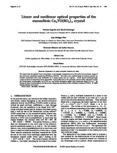
Figure 1. Theoretical and experimental results for χ (2) (ω) of GaAs from Moss et al [3]. The full line in the figure is the calculated spectrum from empirical tight-binding bands while the dotted and dashed lines and the crosses represent experimental measurements from various sources. Moss et al [3] have given detailed references for the experimental data.

Moss et al [3, 4] have carried out empirical tight-binding calculations of the dispersion of the second- and third-order optical constants for zinc-blende crystals. In the first of these (2) (ω) were calculated for GaP, GaAs, papers the finite- and zero-frequency values of χ123 GaSb, InAs and InSb. We have reproduced their results for GaAs in figure 1, in which experimental data have been superimposed. Their approach differs from that of Fong and Shen [10] as they employed three different methods for determining the momentum matrix elements. They were able to show that the use of empirically determined matrix elements gave much better agreement with the measured spectra in the energy ranges where the experimental data existed. From this they concluded that the static limit results of Fong and Shen [10] were an order of magnitude smaller because of an inadequate choice of matrix elements and not due to the local field effect as previously claimed. Their paper also broke new ground as the theoretical expressions for the real and imaginary part of χ (2) (ω) were rearranged to remove the troublesome terms which diverge as ω−3 . The resulting formulae

Optical constants of semiconductors

4693

were presented in a form which could be related to the linear dielectric function, 2 (ω), at ω and 2ω, thus permitting easier correlation between critical points in the bands and structure in χ (2) (ω).

Figure 2. Theoretical predictions of χ (3) (ω) for GaAs (Moss et al [4]). The dashed line (3) (3) component. The represents the χxxxx component and the full line represents the 3 χxyxy figures on the left are from semi-ab-initio bands while those on the right are from empirical tight-binding bands.

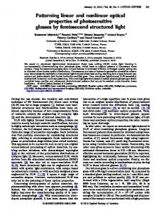
Figure 3. Theoretical predictions of χ (3) (ω) for Si (Moss et al [4]). The presentation of the graphs is the same as figure 2.

After their study of second-order optical properties Moss and co-workers [4] turned their attention to the dispersion of third-order optical constants. They calculated the dispersion, anisotropy and magnitude of χ (3) (ω) in Si, Ge and GaAs using both an empirical tightbinding and a semi-ab-initio band-structure technique. They found the sign of χ (3) (0) to be positive, in agreement with experimental values. A comparison of the results of two different band-structure methods indicated that the dispersion of χ (3) (ω) is extremely sensitive to the details of the energy bands and wavefunctions. Their paper was the first attempt to calculate the dispersion of χ (3) (ω): both nonzero independent elements, given by (3) (3) (ω) ≡ A and χ1212 χ1111 (ω) ≡ B/3, were calculated, and used to determine the anisotropy parameter σ = (B − A)/A which vanishes for an isotropic system. This quantity is of great interest as it is easier to determine experimentally than the absolute value of χ (3) (ω). As in the second-order case, Moss et al [4] rearranged the conventional expressions to remove the divergent ω−4 term, and, as we shall see later, this is not possible within the equation-of-motion formalism. Moss et al [4] were unable to come to any conclusion about

4694

D Hobbs et al

the degree of agreement of the absolute value, χ (3) (ω) , with experiment, as experimental data exist only for two frequencies. Their results are reproduced for GaAs and crystalline Si in figures 2 and 3 respectively. Subsequently Ghahramani et al [7] calculated the dispersion of the first-, second- and third-order optical constants of ZnSe, ZnTe and CdTe using a linear combination of Gaussian orbitals and the formalism developed by Moss et al [3, 4]. They obtained good agreement with experiment and found further evidence that the effects of weak optical transitions are much stronger in second- and third-order spectra than in the linear response function. In a later publication Moss et al [11] applied a semi-ab-initio tight-binding formalism to study the dispersion of χ (3) (ω) in C, Si, Ge, SiC, BP, AlP, AlAs, AlSb, GaP, GaAs, GaSb, InP, InAs and InSb which represent most of group IV and III–V semiconductors. They found that in general χ (3) (ω) is dominated by 3ω- and 2ω-resonances with the direct gap at either the Brillouin zone centre or the E1 critical point. Recently Huang and Ching [12, 13, 14] have published a series of papers on first-, second- and third-order optical properties respectively. They have studied the important group IV, III–V and II–VI compounds using the first-principles orthogonalized linear combination of atomic orbitals (OLCAO) method in the local density approximation. This series of papers uses the expressions derived by Moss et al [3, 4], and represents perhaps the most ambitious approach to calculating the linear and nonlinear optical constants to date. Their results and conclusions are somewhat similar to those of Moss et al [3, 4], although the range of calculations is greater and their analysis is more thorough. Huang and Ching [14] have shown that the validity of Miller’s rule [8] for the ratio between linear and nonlinear susceptibilities is limited to the low-frequency range. Sufficient and accurate conduction band wavefunctions were found to be the crucial ingredients in obtaining accurate third-order spectra. Other topics of particular interest today include structural models of surface reconstruction, the amorphous semiconductors and porous materials. Surface optical spectroscopy has contributed a great deal of understanding concerning the atomic and electronic structure of cleaved semiconductors. The origin of surface optical properties is largely inferred from calculations on simple microscopic structural models. This approach has not reproduced experimental results in detail because of the low level of sophistication of the theory (lack of many-body corrections in the band structure [15]) and the difficulty of modelling real surfaces with simple structural models. McGilp [16] and others have looked beyond this approach by suggesting that second-harmonic generation can be surface specific and may become a useful nondestructive tool for interface studies. This suggestion has prompted Cini [17] to conduct simple model calculations of second-harmonic generation from interfaces, addressing the difficult combination of surface physics and nonlinear optics. The elaborate geometry of realistic surface reconstructions (see, for example, Shkrebtii and Del Sole [18] for a discussion of the Si(100) surface) generally requires a large number of atomic sites. These materials defeat the conventional band-structure methods for realistically calculating nonlinear coefficients. In an attempt to meet the need for new methods for large systems, we have developed the equation-of-motion method for calculating linear and nonlinear optical properties. In the next section we shall review this method, particularly its application to electronic properties. Following this, the general formalism will be presented, and finally explicit expressions for first-, second- and third-order optical properties will be given together with some preliminary results. Because the experimental data are often rather fragmentary and unreliable, we shall concentrate on showing the consistency of the new method with those it is designed to extend.


4695

3. Background on the equation-of-motion method Since the paper of Alben et al [19], the equation-of-motion method has been used to study a variety of different problems. Weaire and Williams [20] used the method to investigate the Anderson localization problem, and they were able to establish an efficient formalism for studying large numbers of atoms. Weaire and Srivastava [21] later refined the method and were then able to identify the Anderson transition. Kramer and Weaire [22] and later Kramer et al [23] showed how the method could be used to determine the conductivity of disordered systems. We have also found the method useful for studying other properties, such as the sign of the Hall coefficient [24] and state densities for large structural models of amorphous semiconductors. A comparative study by Bose [25] of the equation-of-motion and recursion [26] methods suggested that, while similar results were obtained, the recursion method was considerably faster. However, a further detailed comparison was made between the two methods by Weaire and O’Reilly [27] in terms of flexibility, efficiency and transparency of interpretation. They were able to show how the more physically transparent equationof-motion method could be adapted to give comparable efficiency to that of the recursion method. Following the initial developments outlined above, the method has been applied to realistic models of amorphous silicon to calculate properties such as density of states [28] [29], spectral functions [29], diffusivity [30], conductivity [30] and linear optical properties [31, 32]. Recently, massively parallel calculations of the electronic structure of nonperiodic microcrystallites of transition metal oxides have been performed [33]. In this paper the potential of the equation-of-motion method becomes apparent in calculations performed on a structural model of almost half a million atoms. This computation is equivalent to an n × n eigenvalue problem where n ∼ 2 500 000. The equation-of-motion method was originally developed by Alben et al [19] to calculate the density-of-states and spectral functions of large (∼8000 atoms) three-dimensional alloy models. In their paper they solved the time-dependent Schrödinger equation numerically for a time interval determined by the desired energy resolution. They then Fourier analysed the resulting time dependence to obtain the spectrum of the finite model, broadened with a resolution function whose width was predetermined. It should be mentioned at this point that Prelovˇsek [34] pioneered a similar approach to study diffusion in the Anderson model of a disordered system. The basic idea of the paper was to simulate directly the quantum mechanical diffusion of a particle with well defined energy, and to extract quantities such as conductivity and participation ratio from the evolution of an initial state which is localized. 4. The equation-of-motion method The equation-of-motion method generates a specific electronic state 9(t) by numerical integration of the Schrödinger equation ∂ 9(t) = H 9(t) (1) ∂t from a randomly chosen initial state. In the most elementary case, the coefficients in the expansion of the initial state in some basis are random phase factors, eiφn . In calculating optical properties of semiconductors such states are separately specified for the valence and conduction bands, as described below. Time-dependent expressions involving matrix elements between such states must be integrated to yield values of the optical constants ih ¯

4696

D Hobbs et al

as a function of frequency. The equivalence of the equation-of-motion expressions to the standard expressions may be demonstrated by expanding the state 9(t) in terms of energy eigenstates: X 9(t) = (2) an e−iEn t/¯h n . n

The original use of such a method [19] was for the electronic density of states, g(ω), where E =h ¯ ω, in terms of the expression Z T

Re g(ω) = lim dt eiωt e−ηt 9(0) 9(t) . (3) π T →∞ 0 Substitution of the form (2) reduces this to X 2 η an (4) g(ω) = 2 + (ω − E /¯ 2 π(η n h) ) n which approaches the familiar expression X 2 an δ ω − En g(ω) = h ¯ n in the limit η → 0. The expansion coefficients, an , like those in the expansion of the initial state, are random variables [23]. To average over the consequent fluctuations one may either use a large ensemble of different initial states, or, as in (3), use a finite Lorentzian broadening parameter η. In the case of optical properties, more than one initial state is needed and these states are confined to the subspaces of the valence and conduction bands by using a filtering technique [28]. Here this is performed within the empirical tight-binding formalism. These wavefunctions may be used to evaluate matrix elements of the momentum operator and appropriate combinations of these matrix elements may then be Fourier transformed to give approximate values for the required optical constants. The preliminary calculation in which the wavefunctions are modified to exclude eigenfunctions outside the chosen ranges of energy [24] uses the filter function Emax t iE0 t 1 sin exp . (5) f (t) = πt h ¯ h ¯ This confines the wavefunction to the required energy eigenfunction components; the resulting electron wave packet is then drawn from an energy range of 2Emax . The spectrum may be broadened, in order to smooth out the effects of a finite model, as discussed in connection with the calculation of the density of states. In this paper we shall use the semi-empirical tight-binding formalism of Vogl et al [35], in which we have introduced a cut-off between first- and second-nearest neighbours. This scheme is an extension of the tight-binding method of Slater and Koster [36]. In the theory the off-diagonal matrix elements of the Hamiltonian scale according to the d −2 rule of Harrison [37]. When dealing with amorphous materials we simply replace the d −2 parameter for the crystal with that of the amorphous material. The tight-binding scheme of Vogl et al [35] is an ad hoc improvement on that of Slater and Koster [36]. They introduce a somewhat artificial excited s∗ state on each atom, in order to achieve a proper description of the unoccupied anti-bonding lower conduction bands. The interaction matrix elements of the momentum operator are calculated using the commutation relation between the Hamiltonian and position operator in a particular Cartesian direction. mi mi X x [Haa 00 xa 00 a 0 − xaa 00 Ha 00 a 0 ] [H, x] = (6) Paa 0 = h ¯ h ¯ a 00


4697

where a, a 0 and a 00 range over the valence and conduction band states. Only on-site terms have been estimated in the position operator, and its diagonal term is the mean position of each atomic site relative to the origin in the appropriate direction. The only nonzero off-diagonal terms are hs|x|px i and hs∗ |x|px i, i.e. the overlap of the s and s∗ orbitals with the px orbital. These off-diagonal terms are obtained by a fit to bulk optical properties and we have used the following for GaAs [38] and Si [39] ˚ hs∗ |x|px iGaAs = 0.1058 A; ˚ hs|x|px iSi = 0.27 A; ˚ respectively: hs|x|px iGaAs = 0.0265 A; ∗ ˚ hs |x|px iSi = 1.08 A. 5. The dielectric function Weaire et al [31, 32] have used this method to calculate the imaginary part of the dielectric function using both a plane-wave basis [31] and a tight-binding basis set [32]. The calculation was carried out first on a 216-atom model of amorphous silicon (a-Si) [40] and subsequently on models of 1728 atoms of a-Si [41] and 1995 atoms of hydrogenated a-Si (a-Si:H) [42]. For the linear optical properties the following expression for the imaginary part of the dielectric function has been obtained within the equation-of-motion formalism: i ¯ 2 Im lim T −1 2 = π −1 GE −2h T →∞ h ¯ Z T Z

(−i/¯h)(E+iη)t ∞ 0 0 0 (i/¯h)(E+iη)t 0 × dt c(t) P v(t) e dt v(t ) P c(t ) e (7) 0

t

−1

where G = 2 (2πe/m) , ω is the frequency, P is a component of the momentum operator in a particular direction, m and e are the mass and charge respectively of an electron, is the volume of the system and v represents a state confined to the subspace of the valence and c to that of the conduction band. As in (3), η is a Lorentzian broadening parameter, and, as will be seen later, it is included in all of our calculations for optical constants. We use the expressions of Moss et al [3, 4] for nonlinear optical properties but we have modified them by replacing E by E + iη. One may show [31, 32] that expression (7) for the dielectric function is equivalent to the conventional expression involving sums over energy eigenstates by again expanding the time-dependent vectors as in equation (2), distinguishing between valence and conduction band states: X −iEi t/¯h i v(t) = αi e (8) 2

i

X c(t) = βj e−iEj t/¯h j .

(9)

j

After substituting these expansions into expression (7) one finds that most of the resulting products are associated with complex exponentials which average to zero as T → ∞ leaving the conventional expression, apart from fluctuations due to the random initial conditions, discussed above. We have used the equation-of-motion method to calculate the dielectric function for 216-atom models of crystalline and amorphous silicon and GaAs. The finite size of the models used gives rise to detailed structure on the scale 0.2 eV or less, which is of no physical interest. We therefore use a broadening parameter of magnitude 0.27 eV which has the effect of smoothing the results on this scale. The results diverge at low energies because of a finite density of states in the band-gap region, associated with the broadening parameter η and a finite integration time for Schrödinger’s equation. The results, depicted

4698

D Hobbs et al

Figure 4. The dimensionless 2 (ω) for (a) crystalline and (b) amorphous silicon is shown with experimental results [49] superimposed. The numerical results were calculated using the equation-of-motion method and an sps∗ basis. The broadening parameter was 0.0272 eV and four special k-points [50] were used with 216-atom models.

in figures 4(a), 4(b) and 5 for Si (crystalline and amorphous) and GaAs respectively, show quite reasonable behaviour when compared to experimental data [4], which suggests that the tight-binding model should provide a good guide for nonlinear optical properties. 6. Second order For second-order nonlinear optical properties the susceptibility tensor for cubic systems has been obtained from standard perturbation theory by Moss et al [3]. It has been demonstrated by Aspnes [43] that only virtual-electron transitions, i.e. transitions between one valence band and two excited conduction band states (v–c–c0 ), give a significant contribution to the second-order tensor. The virtual-hole contribution, involving transitions between two valence band states and a conduction band state (v–v0 –c), was shown to be negative and more


4699

Figure 5. The dimensionless 2 (ω) for GaAs is shown with experimental results [51] superimposed. The numerical results were calculated using the equation-of-motion method and an sps∗ basis. The broadening parameter was 0.0136 eV and four special k-points [50] were used with a 216-atom model.

than an order of magnitude smaller than the virtual-electron contribution for the materials considered here. In this paper we follow the example of Moss et al [3] and ignore the virtual-hole contribution, in order to make a direct comparison with their results. Using the equation-of-motion method we have obtained expression (A1) which is listed in appendix A. The validity of this expression may be demonstrated by expanding it in terms of sums over eigenstates [44], as explained above. This shows that it is equivalent to the expression of Moss et al [3], in the sense discussed at the beginning of section 4. 6.1. Discussion of results for χ (2) Many band-structure calculations for χ (2) (ω) (Moss et al [3], Huang and Ching [13] and Fong and Shen [10]) already exist for important semiconductor materials. Here we shall demonstrate that the equation-of-motion method may also be used to calculate the secondorder spectra. With the recent interest in surface second-harmonic generation [45] such a novel approach may prove invaluable in the future. The calculations presented here are similar to those of Moss et al [3]. The results presented in their paper are for full bandstructure calculations in the irreducible wedge of the Brillouin zone. (2) (which is χ (2) (ω) has only one independent component which is taken to be χxyz (2) equivalent to χ111 (2ω) used by Fong and Shen [10]) and xyz implies that the appropriate components of the momentum operator are calculated. Our approach is somewhat simplified (2) using four special k-points in the full Brillouin zone in that we calculate the component χxyz and a 216-atom structural model. The results are presented in figure 6 and give reasonable agreement with those of Moss et al [3]. In the energy range 0–0.8 eV the curve diverges as

4700

D Hobbs et al

(2) Figure 6. χxyz (ω) for GaAs. Calculated using the equation-of-motion method and an sps∗ basis. The broadening parameter was 0.0272 eV and four special k-points [50] were used with a 216-atom model. The corresponding results of Moss et al [3] were divided by a factor of two to aid comparison, and are superimposed on the graph.

E −3 due to the prefactor in expression (A1). Other methods of calculation do not suffer from this problem. Moss et al [3] have been able to rearrange the conventional expression using partial fractions and found that the equation was not divergent as E → 0. When using the equation-of-motion formalism one is restricted to using the conventional expression because of the requirement that specific energy denominators should be generated from the integral terms. Our results are of the same order of magnitude as those of Moss et al [3], although relative peak strengths vary somewhat. One should remember that this calculation represents only a simplistic approach, sufficient to convince the reader of the validity of the method. 7. Third order The next obvious step is to see if we can extend this method to calculate the third-harmonic spectrum for some large structural models for which the conventional methodology is yet more cumbersome. We will take amorphous silicon as an example. The most widely used model for amorphous silicon is that of Wooten et al [40] and consists of 216 atoms. To calculate the third-harmonic spectrum of such a model using the conventional approach of sums over eigenstates is simply beyond the capabilities of modern computers. Again following the formalism of Moss et al [4] we attempt to simulate the five physically distinct contributions to χ (3) using the equation-of-motion method. The five contributions are a virtual-electron, three virtual-hole and a three-state term. The virtualelectron term corresponds to the excitation of an electron from the valence band to three


4701

Figure 7. The five physically distinct contributions to χ (3) (ω) (from Moss et al [4]).

successive conduction bands and finally back to the valence band (see figure 7(a)) and we obtain expression (B1), listed in appendix B, within the equation-of-motion formalism. We refer the reader to other work [44] where it is argued that these time-dependent expressions are equivalent to those obtained by Moss et al [4]. Next we must consider the virtual-hole terms. The first virtual-hole term is analogous to the virtual-electron term above: it involves the excitation of a conduction band hole through three successive valence states and finally back to the conduction band (see figure 7(b)). The other two virtual-hole terms correspond to the successive excitation of both an electron and a hole (see figures 7(c) and 7(d)). Rather than reproducing the virtual-hole expressions explicitly one can use table 1 to convert the virtual-electron expression to virtual-hole expressions. This table is analogous to that given by Moss et al [4] for the conventional expressions, and the necessary substitutions for the matrix elements are indicated. The overall sign factor is given in the last column. Finally the three-state term is depicted in figure 7(e) for a one-particle system. This term has a slightly different structure to that of the other third-order terms, and so we reproduce the expression explicitly in appendix B. The demonstration of the equivalence of expression (B2) to its counterpart [4] is similar to that in the case of the virtual-electron process. However, the three-state term is somewhat simplified as the integral labelled S is no longer nested within the integral H , as it was for the virtual-electron and virtual-hole terms.

4702

D Hobbs et al Table 1. Table for converting the virtual-electron term into virtual-hole terms. f (t)

G(t)

H (t)

S(t 0 )

Overall sign

Virtual electron

c(t) P c0 (t)

0 0 v(t ) P c(t )

c0 (t 0 ) P c00 (t 0 )

c00 (t 00 ) P v(t 00 )

+

Virtual

00 hole v (t) P v(t) 0

c(t) P c (t)

0 v (t) P v(t)

0 0 v(t ) P c(t )

0 0 v(t ) P c(t )

0 0 v(t ) P c(t )

v 0 (t 0 ) P v 00 (t 0 ) v 0 (t 0 ) P v(t 0 )

0 0 0 c(t ) P c (t )

c(t 00 ) P v 0 (t 00 ) c0 (t 00 ) P v 0 (t 00 )

0 00 0 00 c (t ) P v (t )

−

+ −

(3) Figure 8. χxxxx (ω) for crystalline GaAs. Calculated using the equation-of-motion method and ∗ an sps basis. The broadening parameter was 0.0136 eV and the special k-point of Baldereschi [52] was used with a 216-atom model. The corresponding results of Moss et al [4] were divided by a factor of two to aid comparison, and are superimposed on the graph.

7.1. Discussion of results for χ (3) The number of full band-structure calculations for third-order nonlinear susceptibility tensors χ (3) (ω) is extremely small. In recent years two detailed papers on the subject have appeared (Moss et al [4] and Ching and Huang [14]) in which full band-structure calculations for group IV, III–V and II–VI crystalline semiconductors have been carried out. The experimental situation is far worse: measurements are typically made at only one wavelength, and so far there is little information (see Burns and Bloembergen [2]) on the dispersion relations available for comparison with the calculated results. The situation for amorphous semiconductors is even graver, with no realistic theoretical calculations, as large structural models are required. We are aware of only one set of experimental data, measured by Moss et al [46], where a comparison is made between crystalline and amorphous silicon at only one wavelength.


4703

(3) Figure 9. χxxxx (ω) for crystalline and amorphous silicon. The presentation of the graphs is the same as in figure 8. The corresponding crystalline Si data from Moss et al [4] have again been divided by a factor of two and are superimposed for comparison.

The object of this section is to make a comparison of the dispersion of χ (3) (ω) for crystalline and amorphous silicon. We have also calculated χ (3) (ω) for GaAs and our results compare favourably with those of Moss et al [4]. For third-harmonic generation there is only a single frequency present and so χ (3) (ω) will be symmetric in the last three indices. In addition, for cubic materials, all of the (x, y, z) Cartesian directions are equivalent and so there are only two nonzero independent elements of χ (3) (ω) (see Burns and Bloembergen (3) (3) (3) (3) (ω) and B ≡ 3χxyxy (ω) = 3χxyyx (ω) = 3χxxyy (ω). In this paper [2]), namely A ≡ χxxxx (3) we have only attempted to simulate the first component, χxxxx (ω), as we are interested in a comparison with the experimental data of Moss et al [46], who found that at an energy of 1.17 eV (1.06 µm) the absolute value of χ (3) (ω) was smaller by about 33% in ion-implanted amorphous silicon than in crystalline silicon. We present results for GaAs in figure 8, which were calculated using one special kpoint and a 216-atom structural model. Data have not been shown below 0.4 eV because the results diverge as E −4 as E → 0 due to the prefactor in expressions (B1) and (B2). The remaining data agree quite well with those of Moss et al [4] although the magnitude of our results is somewhat lower. In figure 9 the comparison between crystalline and amorphous silicon is presented, the crystalline results being equivalent to those of Moss et al [4]. The comparison is at first rather striking. The main peak of the amorphous data is centred just above 0.9 eV, about 0.1 eV below the main crystalline peak. Our results do not, however, conflict with the measurements of Moss et al [46], since their measurements were made at 1.17 eV, and at this energy the equation-of-motion data are comparable for the two materials, although the results are not sufficiently accurate to predict small differences.

4704

D Hobbs et al

8. Conclusion We have presented various preliminary results of an alternative method of calculating the optical properties of solids in cases which defeat the conventional band-structure approaches. Agreement with older methods, in the case of small unit cells, seems sufficient to encourage further development. We have examined the relationships between the expressions used for optical constants in the equation-of-motion method and the standard expressions derived through time-dependent perturbation theory. Zuchuat [47] has developed a set of rules, based on a diagrammatic approach, for constructing the equation-of-motion expressions, and showed that for the nonlinear constants, the expressions (A1) and (B1) used for calculating χ (2) and χ (3) arise from exploiting total symmetry of the standard expressions under exchange of pairs of photon lines. This total symmetry is strictly applicable only in the complete absence of absorption; however the widths of the lines in the solid are so narrow in comparison with the resolution claimed for the results of the equation-of-motion calculations that it is reasonable to make the approximation. As a final note we should add that Morgan and Okumu [48] have very recently used a random-phase approach to estimate χ (3) (ω) for a-Si. Their results seem consistent with those shown here in figure 9. Acknowledgments We would like to express out gratitude to Professor J E Sipe for permission to reproduce figures from his publications. One of the authors (DH) would like to thank Professor G J Morgan for useful discussions. We also wish to thank John McGilp and all of the members of Esprit actions EPIOPTIC and EASI for their help and advice. Appendix A. Second order

χV(2).E. (ω)

Z T Z i e 3 1 dk = f1 (t)G1 (t)H1 (t) dt lim 2 2 mω T →∞ h ¯ T BZ 4π 3 0 Z T Z T + f2 (t)G2 (t)H2 (t) dt + f3 (t)G3 (t)H3 (t) dt 0

where

0

f1 (t) = c(t) P c0 (t) e−(i/¯h)(E+iη)t Z −∞

0 0 0 −(i/¯h)(E+iη)t 0 0 G1 (t) = dt c (t ) P v(t ) e t Z ∞

0 0 (i/¯h)(2E+2iη)t 0 0 H1 (t) = dt v(t ) P c(t ) e t 0 (i/¯h)(2E+2iη)t

f2 (t) = c(t) P c (t) e Z −∞

0 0 0 −(i/¯h)(E+iη)t 0 0 G2 (t) = dt c (t ) P v(t ) e t Z −∞

0 0 −(i/¯h)(E+iη)t 0 0 H2 (t) = dt v(t ) P c(t ) e t 0 −(i/¯h)(E+iη)t

f3 (t) = c(t) P c (t) e

(A1)

Optical constants of semiconductors Z ∞

0 0 0 (i/¯h)(2E+2iη)t 0 0 dt c (t ) P v(t ) e G3 (t) = t Z −∞

0 0 −(i/¯h)(E+iη)t 0 0 H3 (t) = dt . v(t ) P c(t ) e

4705

t

Appendix B. Third order The virtual-electron term is Z T Z 1 e 4 i dk (3) f1 (t)G1 (t)H1 (t) dt χV .E. (ω) = lim 3 3 mω T →∞ h ¯ T BZ 4π 3 0 Z T Z T + f2 (t)G2 (t)H2 (t) dt + f3 (t)G3 (t)H3 (t) dt 0 0 Z T + f4 (t)G4 (t)H4 (t) dt 0

where

f1 (t) = c(t) P c0 (t) e−(i/¯h)(E+iη)t Z ∞

0 0 (i/¯h)(3E+3iη)t 0 0 G1 (t) = dt v(t ) P c(t ) e t Z −∞

0 0 00 0 −(i/¯h)(E+iη)t 0 H1 (t) = S1 (t 0 ) dt 0 c (t ) P c (t ) e t Z −∞

00 00 00 −(i/¯h)(E+iη)t 00 00 S1 (t 0 ) = dt c (t ) P v(t ) e t0 0 (i/¯h)(3E+3iη)t

f2 (t) = c(t) P c (t) e Z −∞

0 0 −(i/¯h)(E+iη)t 0 0 G2 (t) = dt v(t ) P c(t ) e t Z −∞

0 0 00 0 −(i/¯h)(E+iη)t 0 H2 (t) = S2 (t 0 ) dt 0 c (t ) P c (t ) e t Z −∞

00 00 00 −(i/¯h)(E+iη)t 00 00 S2 (t 0 ) = dt c (t ) P v(t ) e t0

f3 (t) = c(t) P c0 (t) e−(i/¯h)(E+iη)t Z −∞

0 0 −(i/¯h)(E+iη)t 0 0 G3 (t) = dt v(t ) P c(t ) e t Z ∞

0 0 00 0 (i/¯h)(3E+3iη)t 0 H3 (t) = S3 (t 0 ) dt 0 c (t ) P c (t ) e t Z −∞

00 00 00 −(i/¯h)(E+iη)t 00 00 S3 (t 0 ) = dt c (t ) P v(t ) e t0 0 −(i/¯h)(E+iη)t

f4 (t) = c(t) P c (t) e Z −∞

0 0 −(i/¯h)(E+iη)t 0 0 G4 (t) = dt v(t ) P c(t ) e t Z ∞

0 0 00 0 −(i/¯h)(E+iη)t 0 H4 (t) = S4 (t 0 ) dt 0 c (t ) P c (t ) e t

(B1)

4706

D Hobbs et al Z ∞

00 00 00 (i/¯h)(3E+3iη)t 00 00 dt . c (t ) P v(t ) e S4 (t 0 ) = t0

The three-state term is Z T Z 1 e 4 i dk (3) χthree−state (ω) = f1 (t)G1 (t)H1 (t)S1 (t) dt lim 3 3 mω T →∞ h ¯ T BZ 4π 3 0 Z T Z T − f2 (t)G2 (t)H2 (t)S2 (t) dt + f3 (t)G3 (t)H3 (t)S3 (t) dt 0 0 Z T − f4 (t)G4 (t)H4 (t)S4 (t) dt 0

where

f1 (t) = c(t) P v 0 (t) e−(i/¯h)(E+iη)t Z ∞


0 0 0 0 −(i/¯h)(E+iη)t 0 0 H1 (t) = dt v (t ) P c (t ) e t Z −∞

0 0 0 −(i/¯h)(E+iη)t 0 0 S1 (t) = dt c (t ) P v(t ) e t

0 0 −(i/¯h)(E+iη)t f2 (t) = v (t) P c (t) e Z ∞

0 0 0 (i/¯h)(3E+3iη)t 0 0 G2 (t) = dt c (t ) P v(t ) e t Z −∞

0 0 0 −(i/¯h)(E+iη)t 0 0 H2 (t) = dt c(t ) P v (t ) e t Z −∞

0 0 −(i/¯h)(E+iη)t 0 0 S2 (t) = dt v(t ) P c(t ) e t

0 −(i/¯h)(E+iη)t f3 (t) = c (t) P v(t) e Z ∞


0 0 0 0 −(i/¯h)(E+iη)t 0 0 H3 (t) = dt v (t ) P c (t ) e t Z −∞

0 0 0 −(i/¯h)(E+iη)t 0 0 S3 (t) = dt c(t ) P v (t ) e t

−(i/¯h)(E+iη)t f4 (t) = v(t) P c(t) e Z ∞

0 0 0 (i/¯h)(3E+3iη)t 0 0 G4 (t) = dt c (t ) P v(t ) e t Z −∞

0 0 0 −(i/¯h)(E+iη)t 0 0 H4 (t) = dt c(t ) P v (t ) e t Z −∞

0 0 0 0 −(i/¯h)(E+iη)t 0 0 S4 (t) = dt . v (t ) P c (t ) e t

(B2)


4707

References [1] [2] [3] [4] [5] [6] [7] [8] [9] [10] [11] [12] [13] [14] [15] [16] [17] [18] [19] [20] [21] [22] [23] [24] [25] [26] [27] [28] [29] [30] [31] [32] [33] [34] [35] [36] [37] [38] [39] [40] [41] [42] [43] [44] [45] [46] [47] [48] [49] [50] [51] [52]

Chang R K, Ducuing J and Bloembergen N 1965 Phys. Rev. Lett. 15 415 Burns W K and Bloembergen N 1971 Phys. Rev. B 4 3437 Moss D J, Sipe J E and van Driel H M 1987 Phys. Rev. B 36 9708 Moss D J, Ghahramani E, Sipe J E and van Driel H M 1990 Phys. Rev. B 41 1542 Butcher P N and McLean T P 1963 Proc. Phys. Soc. 81 219 Butcher P N and McLean T P 1964 Proc. Phys. Soc. 83 579 Ghahramani E, Moss D J and Sipe J E 1991 Phys. Rev. B 43 9700 Bassani F and Pastori Parravincini G 1973 Electronic States and Optical Transitions in Solids (Oxford: Pergamon) Joannopoulos J D and Cohen M L 1973 Phys. Rev. B 7 2644 Fong C Y and Shen Y R 1975 Phys. Rev. B 12 2325 Moss D J, Ghahramani E and Sipe J E 1991 Phys. Status Solidi 164 587 Huang Ming-Zhu and Ching W Y 1993 Phys. Rev. B 47 9449 Huang Ming-Zhu and Ching W Y 1993 Phys. Rev. B 47 9464 Ching W Y and Huang Ming-Zhu 1993 Phys. Rev. B 47 9479 Del Sole R and Fiorino E 1984 Phys. Rev. B 29 4613 McGilp J F 1989 J. Phys.: Condens Matter 1 SB85 Cini M 1991 Phys. Rev. B 43 4792 Shkrebtii A I and Del Sole R 1993 Phys. Rev. Lett. 70 2645 Alben R, Blume M, Krakauer H and Schwartz L 1975 Phys. Rev. B 12 4090 Weaire D and Williams A R 1977 J. Phys. C: Solid State Phys. 10 1239 Weaire D and Srivastava V 1977 Commun. Phys. 2 73 Kramer B and Weaire D 1978 J. Phys. C: Solid State Phys. 11 L5 Kramer B, MacKinnon A and Weaire D 1981 Phys. Rev. B 12 6357 Weaire D and Hobbs D 1993 Phil. Mag. Lett. 68 265 Bose S K 1984 Phil. Mag. B 49 631 Haydock R, Heine V and Kelly M J 1972 J. Phys. C: Solid State Phys. 5 2845 Weaire D and O’Reilly E P 1985 J. Phys. C: Solid State Phys. 18 1401 Hickey B J, Morgan G J Weaire D L and Wooten F 1985 J. Non-Cryst. Solids 77 + 78 67 Hickey B J and Morgan G J 1986 J. Phys. C: Solid State Phys. 19 6195 Hickey B J, Birr J N and Morgan G J 1990 Phil. Mag. Lett. 61 161 Weaire D, Hickey B J and Morgan G J 1991 J. Phys.: Condens Matter 3 9575 Weaire D, Hobbs D, Morgan G J, Holender J M and Wooten F 1993 J. Non-Cryst. Solids 164–166 877 Michalewicz M T 1994 Comput. Phys. Commun. 13–23 79 Prelovˇsek P 1984 Phil. Mag. B 49 631 Vogl P, Hjalmarson H P and Dow J D 1983 J. Phys. Chem. Solids 44 365 Slater J C and Koster G F 1954 Phys. Rev. 94 1498 Harrison W A 1989 Electronic Structure and the Properties of Solids (New York: Dover) Del Sole R 1992 private communications Del Sole R and Girlanda R 1993 Phys. Rev. B 48 11 789 Wooten F, Winer K and Weaire D 1985 Phys. Rev. Lett. 54 1392 Holender J M and Morgan G J 1991 J. Phys.: Condens. Matter 3 7241 Holender J M, Morgan G J and Jones R 1993 Phys. Rev. B 47 3991 Aspnes D E 1972 Phys. Rev. B 6 4648 Hobbs D 1995 PhD Thesis Trinity College, University of Dublin McGilp J F 1990 J. Phys.: Condens. Matter 2 7985 Moss D J, van Driel H M and Sipe J E 1986 Appl. Phys. Lett. 48 1150 Zuchuat O 1994 Diploma Thesis Ecole Polytechnique Federale, Lausanne Morgan G J and Okumu J 1996 private communications (to be published) Pierce D T and Spicer W E 1972 Phys. Rev. B 5 3017 Chadi D J and Cohen M L 1973 Phys. Rev. B 8 5747 Philipp H R and Ehrenreich H 1963 Phys. Rev. 129 1550 Baldereschi A 1973 Phys. Rev. B 7 5212