the computational measure of uniformity - Semantic Scholar

THE FLORIDA STATE UNIVERSITY COLLEGE OF ARTS AND SCIENCES

THE COMPUTATIONAL MEASURE OF UNIFORMITY

BY

YAOHANG LI

A Thesis submitted to the Department of Computer Science In partial fulfillment of the requirements for the degree of Master of Science

Degree Awarded: Summer Semester, 2000

The members of the Committee approve the thesis of Yaohang Li defended on 7/17/2000.

Michael Mascagni Professor Directing Thesis

Kyle Gallivan Committee Member

David Banks Committee Member

Approved:

Theodore P. Baker, Chair, Department of Computer Science

In memory of my paternal grandmother, Weishi Li (1924 - 1998).

iii

ACKNOWLEDGEMENTS

I would like to express my sincere thanks and appreciation to my advisor, Dr. Michael Mascagni for his continuous encouragement and kind help in my research and study. Also, I give thanks to all my other graduation committee members, Dr. Kyle Gallivan and Dr. David Banks, for their helpful comments and advice.

I appreciate the help from our research group, especially Dr. Aneta Karaivanova, Dr. Chi-Ok Hwang, Wenchang Yan’s creative discussion and Ethan Kromhout’s help for correcting my grammar.

I express my deepest gratitude and respect to my parents in China. Also, in heart, I will always remember all of my friends who supported me and helped me, especially during my difficulties.

Above all, thanks God’s awesome love and guidance for me.

iv

TABLE OF CONTENTS LIST OF TABLES ............................................................................................................vii LIST OF FIGURES..........................................................................................................viii ABSTRACT .......................................................................................................................ix CHAPTER 1. INTRODUCTION ....................................................................................... 1 1.1

Introduction............................................................................................................ 1

1.2

Monte Carlo Method and quasi-Monte Carlo Method .......................................... 2

1.3

Definition of Discrepancy...................................................................................... 3

1.4

Definition of a Quasirandom Sequence ................................................................. 4

1.5

The Koksma-Hlawka Inequality............................................................................ 5

1.6

Wozniakowski’s Identity ....................................................................................... 6

1.7

Applications of Computational Measure of Uniformity........................................ 7

CHAPTER 2. COMPUTING THE EXACT STAR DISCREPANCY DN*........................ 8 2.1

A General Approach to Star Discrepancy, D N*...................................................... 8

2.2

A Method of Computing Discrepancy DN* Based on Orthants ........................... 10

2.2.1 Definition of Orthant ......................................................................................... 10 2.2.2 Basic Idea .......................................................................................................... 12 2.2.3 Algorithm Based on Orthants for Computing DN* ............................................ 12 v

2.3

Improvement of the Method Based on Orthants.................................................. 15

2.4

Numerical Results................................................................................................ 18

CHAPTER 3. AN APPROXIMATE ALGORITHM FOR COMPUTING DN* ............... 21 3.1

Introduction.......................................................................................................... 21

3.2

The Approximate Algorithm Using Random Walks ........................................... 22

3.2.1 Random Walks .................................................................................................. 22 3.2.2 Implementation.................................................................................................. 23 3.2.3 Numerical Results ............................................................................................. 24 3.2.4 Discussion.......................................................................................................... 27 CHAPTER 4. COMPUTING THE L2 DISCREPANCY.................................................. 29 4.1

The Formula for Computing the L2 Discrepancy ................................................ 29

4.2

The Algorithm for Computing L2 Discrepancy ................................................... 30

4.3

Numerical Results................................................................................................ 30

4.4

Approximation Method for the L2 Discrepancy .................................................. 31

CHAPTER 5. APPLICATION OF DISCREPANCY COMPUTATION ALGORITHMS ........................................................................................................................................... 33 CHAPTER 6. SUMMARY............................................................................................... 36 6.1

Conclusion ........................................................................................................... 36

6.2

Future Work ......................................................................................................... 37

REFERENCES.................................................................................................................. 39 BIOGRAPHICAL SKETCH ............................................................................................ 41

vi

LIST OF TABLES Table 2.1

……………………………………………………………………

19

Table 2.2

……………………………………………………………………

19

Table 3.1

……………………………………………………………………

27

Table 3.2

……………………………………………………………………

27

Table 3.3

……………………………………………………………………

27

Table 4.1

……………………………………………………………………

31

Table 4.2

……………………………………………………………………

31

vii

LIST OF FIGURES Figure 1.1

……………………………………………………………………

5

Figure 2.1

……………………………………………………………………

9

Figure 2.2

…………………………………………………………………… 11

Figure 2.3

…………………………………………………………………… 11

Figure 2.4

…………………………………………………………………… 11

Figure 2.5

…………………………………………………………………… 14

Figure 2.6

…………………………………………………………………… 15

Figure 2.7

…………………………………………………………………… 17

Figure 2.8

…………………………………………………………………… 19

Figure 3.1

…………………………………………………………………… 22

Figure 3.2

…………………………………………………………………… 25

Figure 3.3

…………………………………………………………………… 25

Figure 3.4

…………………………………………………………………… 26

Figure 4.1

…………………………………………………………………… 30

Figure 5.1

…………………………………………………………………… 34

Figure 5.2

…………………………………………………………………… 34

Figure 6.1

…………………………………………………………………… 37 viii

ABSTRACT

The quasi-Monte Carlo method has a faster convergence rate than does the ordinary Monte Carlo method. However, the accuracy of the quasi-Monte Carlo method depends on the uniformity of the quasirandom number sequences used. Discrepancy is an important measure of the uniformity of a sequence; however, the computation of discrepancy is easy to describe but impractical to carry out. In this paper, we discuss and analyze methods for exactly computing the L∞ discrepancy, an approximate method for the L∞ discrepancy based on random walks, a formula for exactly computing the L2 or mean square discrepancy and some applications of these methods. Finally we present some numerical results and comment on the effectiveness of these methods.

ix

CHAPTER 1 INTRODUCTION 1.1

Introduction

Monte Carlo methods and quasi-Monte Carlo methods provide approximate solutions to a variety of mathematical problems through statistical sampling. They are important techniques for performing simulation, optimization and integration, and form the computational foundation for many fields including transport theory, quantum chromodynamics, and computational finance [16] [17].

In section 1.2 we give a general overview of both the Monte Carlo Method and the quasi-Monte Carlo Method. The definitions of discrepancy and quasirandom sequence are given in section 1.3 and 1.4. We then present, in section 1.5 and 1.6, the Koksma-Hlawka inequality and Wozniakowski’s identity to analyze quasi-Monte Carlo integration. In section 1.7, we discuss applications that require computing the discrepancy. In Chapter 2, we provide a general approach to estimate the exact L∞ star discrepancy and give some computational improvements. Since the exact method is still impractical when the number of points is large or the dimension is high, we propose an approximate method using random walks to estimate the L∞ star discrepancy in Chapter 3. In Chapter 4, we state a formula to compute the L2 star discrepancy. In Chapter 5, we adapt the methods of computing and estimating different discrepancies for analysis of different quasirandom sequences. In this section we provide extensive numerical results. In the last section we summarize our findings and detail plans for future work on this topic. 1

1.2

Monte Carlo Method and quasi-Monte Carlo Method

When using the Monte Carlo method, a set of computational random numbers has to be generated and used to statistically estimate a quantity of interest. The probabilistic convergence rate of this process is known to be O(N-1/2) [1]. Computations using the Monte Carlo method are independent of dimension, which avoids “the curse of dimensionality”. In addition, many Monte Carlo methods allow the treatment of complicated geometries without many of the difficulties encountered in computing with deterministic methods. For this as well as other reasons, it is the only viable computational method for a wide range of problems. Let us assume we wish to estimate a quantity θ with a Monte Carlo method. Assume a statistic θ* can be constructed so that E[θ*] = θ, where E[ ] is the expected value. In addition define the variance of θ* as Var[θ*] = σ2 = E[(θ*-θ)2]. Define

θ N* =

1 N

N

∑θ i =1

* [i ]

as the average of N realizations of θ*. The mean of θ is given by

θ N* = E[θ N* ] = E[θ * ] = θ , and Var[θ N* ] =

σ2 . The standard deviation, or the square root N

of the variance of a random variable, indicates the uncertainty in a Monte Carlo computation. As N increases, the standard error of θ N* ,

σ , goes to 0 as N-1/2. Thus, the N

error, or as it is often called, the standard error of a random s ample with N independent realizations, is O(N-1/2).

A serious drawback of the Monte Carlo method is this slow rate of convergence. In order to accelerate the convergence rate of the Monte Carlo method, several techniques can be applied. Variance reduction methods, such as antithetic variates, control variates, stratification and importance sampling, reduce the variance, σ2. An alternate method is 2

the quasi-Monte Carlo method, which uses quasirandom (subrandom) sequences that are highly uniform instead of the usual random or pseudorandom numbers. While pseudorandom numbers are constructed to imitate the behavior of truly random sequences, the members of a quasirandom sequence are deterministic, and achieve equidistribution often at the cost of correlation and independence. Therefore, quasiMonte Carlo methods can often converge more rapidly, at a rate of O(N-1(logN)k), for some k [1]. This accelerated convergence rate is due to the fact that quasirandom numbers are more evenly distributed than random number. The measure used to describe this uniformity is called the discrepancy.

1.3

Definition of Discrepancy

We use discrepancy to measure the uniformity of a sequence of points. For a sequence of N points X = {x0, … ,xN-1} in the d-dimensional unit cube Id, define RN ( J ) = µ X ( J ) − µ ( J ) , for any subset J of Id. µ X ( J ) =

# of points in J ∈ [0,1] is the discrete measure of J, i.e., N

the fraction of points of X in J, and µ(J) ∈ [0,1] is the Euclidean measure of J, i.e., the volume of J. Restrict J to be a hyper-rectangular set, then the definitions of discrepancy DN and TN, which are related L∞ norms and L2 norms are: DN = sup | RN ( J ) | , J ∈E

TN = [ ∫

( x , y )∈I 2 d , xi < yi

RN ( J ( x, y )) 2 dxdy ]1 / 2 .

Here E is the set of all hyper-rectangles within the unit cube and hyper-rectangle J can be identified as J = J(x,y) in which the points x and y are antipodal vertices. The overall L∞ discrepancy can be interpreted as the maximum discrepancy of all of the hyperrectangles, whereas TN is a mean square discrepancy [2]. According to the definition, we have the following relation:

3

0 < TN ≤ D N ≤ 1

Because of the difficulty in computing the discrepancy, we restrict the J to those boxes that have one corner at the origin, and we obtain a variant definition of discrepancy called the star discrepancy:

DN* = sup | RN ( J ) | , J ∈E *

TN* = [ ∫ d RN ( J (0, x)) 2 dx]1/ 2 , I

in which E* is the set {J(0,x)}. We also call | RN(J) | the discrepancy of the hyperrectangle J or the discrepancy of point x, where x is the antipodal vertex of J [3]. Note, in one dimension DN* is just the maximal deviation of the empirical distribution of X from the uniform distribution.

A point set whose distribution is far from uniformity will have a high discrepancy; on the contrary, a point set which is distributed evenly will tend to have a low discrepancy. A well-behaved random number generator should have its discrepancy of the same order (for large N) as that of a truly random sequence, which lies between O(N-1/2) and O(N-1/2(loglogN)1/2), according to the law of the iterated logarithm. This holds for both the star and extreme discrepancies [11].

1.4

Definition of a Quasirandom Sequence

An infinite sequence X = {x0, … ,xN-1} is uniformly distributed if lim DN = 0 .

N →∞

A sequence is quasirandom if DN ≤ c(log N ) k N −1 ,

in which c and k are constants that are independent of N, but may depend on the dimension, d [2]. 4

Figure 1.1 shows that a quasirandom sequence (Sobol’ Sequence) has a more uniform appearance than that of a pseudorandom sequence generated by the Scalable Parallel Random Number Generators (SPRNG) library [14].

Figure 1.1: Two-Dimensional Pseudorandom Sequence Vs. Quasirandom Sequence

1.5

The Koksma-Hlawka Inequality

Quasirandom sequences are useful for integration because they lead to much smaller error than standard Monte Carlo integration. The Koksma-Hlawka inequality is the foundation of analyzing quasi-Monte Carlo quadrature error.

Theorem 1.1 (Koksma-Hlawka Theorem) For any sequence X = {x0,…,xN-1} and any function, f, with bounded variation, the integration error ε is bounded as 5

ε [ f ] ≤ V [ f ]DN* . Here V[f] is the total variation of f, in the sense of Hardy-Krause, and DN* is the star discrepancy of sequence X = {x0,…,xN-1}. A good explanation about and a clear proof of the Koksma-Hlawka theorem can be found in [2].

According to the definition of a quasirandom sequence, the quasi-Monte Carlo integration error is therefore:

ε [ f ] ≤ V [ f ]DN* ≤ V [ f ]c(log N ) k N −1 . For this reason, Monte Carlo integration using quasirandom points converges more rapidly, at a rate of O(N-1(logN)k), than Monte Carlo integration using pseudorandom numbers. Note that the Koksma-Hlawka inequality applies for any sequence. Therefore, in this case, the smaller the discrepancy of a sequence, the better it is to minimize the numerical error of quasi-Monte Carlo integration. In addition, this is a deterministic error bound; as opposed to those usually obtain with Monte Carlo method. The rub is that using this bound requires computing DN*.

1.6

Wozniakowski’s Identity

An important theoretical application of TN* is to the average case complexity of a numerical integration.

Theorem 1.2 (Wozniakowski’s Identity) We have E[ε [ f ]2 ] = (TN* ) 2 ,

in which the expectation E is taken with respect to function f distributed according to the Brownian sheet measure [2].

Wozniakowski’s identity shows that discrepancy is a good indicator of the average case performance of numerical integration, while variation, as it appears in the 6

Koksma-Hlawka inequality, is not a typical indicator. The L2 discrepancy, TN* , agrees with the typical error size in quasi-Monte Carlo integration.

1.7

Applications of Computational Measure of Uniformity

Based on the Koksma-Hlawka inequality and Wozniakowski’s identity, we can use the discrepancies DN* and TN* to estimate the error of quasi-Monte Carlo integration and other quasi-Monte Carlo simulations. From the Koksma-Hlawka inequality, we know that the error of the integration is proportional to the discrepancy of the quasirandom sequence used. By analyzing the discrepancy, we can understand the error trend for an integration. Usually, for a specified quasirandom sequence, a theoretical upper bound of its discrepancy might be available. However, in our computational experience, the upper bound of the discrepancy is much larger than the computationally devised discrepancy of a quasirandom sequence. Therefore, by computing the exact value of the discrepancy, we can obtain a better estimate of the error of the quasi-Monte Carlo integration.

The quality of a quasirandom sequence is crucial for the quasi-Monte Carlo method. However, every method of generating quasirandom numbers requires choosing optimal parameters. For example, in generating the Sobol’ sequence, we need to get the direction numbers from each dimension [15]. By analyzing the discrepancy of the sequences generated using different direction numbers, we can empirically determine the “best” direction numbers. Thus, the estimation of the discrepancy can help us find the best generation parameters to provide an optimal quasirandom sequence. In fact, we intend to use our computation discrepancy tools for exactly this purpose.

7

CHAPTER 2 COMPUTING THE EXACT STAR DISCREPANCY DN* In this chapter, we discuss the computation of the exact star discrepancy DN*, some of the technical algorithmic improvements, and numerical results.

2.1

A General Approach to Star Discrepancy, DN*

We now review some formulas and algorithms for computing DN*. The star discrepancy of a set of n points X = {x0,…,xN-1} ∈ Id does not depend on the order of the points. Therefore, in one dimension we can order the points to exploit Niederreiter’s formula, DN* ( x) =

1 2i + 1 + max | xi − |, 2 N 0≤i≤ N −1 2N

assuming that the order is 0 ≤ x0 ≤ … ≤ xN-1≤ 1 [4].

De Clerk [4] proposed a method for the exact calculation of the star discrepancy for d = 2. When d > 2, computing the star discrepancy exactly is regarded to be a difficult task. There seem to have been no publications on this subject until 1993, when Bundschuh and Zhu [5] gave an enumeration algorithm for computing the stardiscrepancy for small d. Somewhat later, Dobkin and Eppstein [3] provided a theoretical method and data structure to compute the orthant discrepancy and half-plane discrepancy. Our analysis of their method follows. 8

It is impossible to write a program that iterates through the uncountably many rectangles J in Id. However, we can enumerate all the rectangles that have an extreme corner at a grid point, which is constructed by the coordinates of all xi ∈ X in all dimensions. Moreover, a rectangle whose sides contain points in X is a candidate for having the maximum discrepancy. Consider the sequence X = {x0, …, xN-1}. For every i ∈ {1 ,…, d}, let 0 = β 0(i ) < β1(i ) < ... < β n(ii ) = 1 , ni ≤ N-1, be the distinct numbers occurring as the i-th coordinates of x0, …, xN-1 together with 0 and 1. Based on β (ij ) at every dimension i, we can divide the hyper-cube Id into many smaller boxes and build up a grid in Id. Figure 2.1 is a two-dimensional example. The unit square is divided into 49 smaller rectangles with the origin at one corner. It is easy to show that only at the grid points of these rectangles can we find the overall maximum discrepancy, i.e., the nongrid points cannot be the location of the maximum discrepancy. Hence, the computation of the star discrepancy computationally reduces to enumerating all of the grid points and finding the maximum discrepancy among the grid points.

Figure 2.1: Grid Points in the Unit Square We define the set Q of all of such grid points: Q = {( j1 ,..., j s ), 0 ≤ ji < ni for 1 ≤ i ≤ s} . For every grid point q ∈ Q and the origin we can construct a hyper-rectangle J(0,q). Suppose there are npq points of X = {x0,…,xN-1} in the hyper-rectangle J(0,q) (including

9

the points on the border) and nbq points of X on the border of J(0,q), then the stardiscrepancy of X can be represented as DN* ( x) = max max{| q∈Q

npq N

− V (q ) |, |

np q − nbq N

− V (q ) |} [9],

where V(q) is the volume of the hyper-rectangle whose antipodal vertices are the origin and the point q. There are at most (N+1)d grid points in the unit cube Id, and so the method of searching all of the grid points will take O(Nd) time.

2.2

A Method of Computing Discrepancy DN* Based on Orthants

2.2.1 Definition of Orthant Section 2.1 shows that only finitely many rectangles (in fact, (N+1)d of them) need to be enumerated to calculate DN*. But we can reduce this search space even further, almost by a factor of N. Consider Figure 2.1 again with the two-dimensional grid points. We discovered that it is not necessary to compute the discrepancy at all the grid points. In Figure 2.2, only the rectangles constructed at grid points in the circle are needed to compute the discrepancy of the rectangle; all the other grid points can be discarded. For a grid point pi, if we can find another grid point pj, which constructs a rectangle having a bigger volume than that of pi, and pk having a smaller one with each of their rectangle containing exactly the same number of points, then the discrepancy of pi is either less than pj or less than pk. Thus, pi cannot be the location of the maximum discrepancy. In Figure 2.2, only 24 grid points need to be considered, while the exhaustive search method needs to process more than twice this number of grid points.

10

Figure 2.2: Grid Points Needed (The grid points needed to compute DN* are shown as open circles. The dots are elements of the sequence xi) In the two-dimensional case, we wish to find a quadrant of the unit square containing the origin and maximizing the discrepancy. The corner of the quadrant will have as its coordinates some of the coordinates of points in {x0, …, xN-1}, but different coordinates may be drawn from different points so the quadrant might not necessarily have any xi at its corner. Such a quadrant is an orthant. Figure 2.3 shows two possible cases of a two-dimensional orthant. Figure 2.4 shows an example of three-dimensional orthants. As a basic characteristic, there is at least one point of X on an orthant’s every border inside Id. Extending this to d dimensions, there must be at least one point at every inner border hyperplane of the d-dimensional orthant.

An orthant with an actual point at the corner

An orthant without an actual point at the corner

Figure 2.3: Two Possible Cases of a 2D Orthant

11

Orthants with 1 point

Orthant with 2 points

Figure 2.4: Example of 3D Orthants 2.2.2 Basic Idea The basic idea for directly computing the discrepancy is to find, for each value of n from 1 to N, the orthants with minimum and maximum area that contain exactly n of the N points. When the box, J, is an orthant, we also call | RN(J) | the discrepancy of orthant J [3]. Finally, the overall discrepancy is the maximum of all the orthant discrepancies.

By Dobkin and Eppstein’s [3] theoretical result, we can get the following time and space complexity analysis.

Theorem 2.1 For any d dimensional point set, we can compute the discrepancy in time O(Nd-1log2N) and space O(NlogN), [3].

2.2.3 Algorithm Based on Orthants for Computing DN* Based on Dobkin and Eppstein’s theoretical idea of computing the orthant discrepancy, we now define an iterative algorithm for computing the star discrepancy using an iteration on orthants containing exactly n points. It is named the 1-to-N algorithm because it searches from the orthants with exactly 1 point to the orthants with exactly N points. Dobkin and Eppstein did not construct an explicit d-dimensional orthant 12

algorithm. Instead, they explicitly detailed the 2-dimensional algorithm and derived their complexity results via induction on dimension. Our own analysis of this induction leads to the explicit algorithms described below.

Algorithm 2.1 [1-to-N] [Initialization] [1] For every dimension i from 1 to d Sort x0, …, xN-1 by their i-th coordinates, respectively, together with 0 and 1. [2] Find all of the orthants that contain exactly 1 point and put them in the orthant array. In this 1-point case, the point is at the corner of the orthant.

[Compute the discrepancy of all possible orthants] [3] For n from 1 to N For every orthant j in the orthant array that contains exactly n points For every dimension i from 1 to d Find the next point whose coordinate is next to the current orthant at this dimension. Include this point and build up a new orthant. If this orthant contains exactly n + 1 points, put the new orthant in the orthant array with n + 1 points. If the new orthant already exists, discard it. Else Find next possible point. Until one finds such a point or reaches the border of the unit cube Id. Compute the discrepancy of the current orthant. Set the current maximum discrepancy.

13

[Finalization] [4] Set the current maximum discrepancy as the overall discrepancy.

Figure 2.5 gives a two-dimensional example of the procedure of computing all of the orthants containing exactly 1 to 4 points.

Orthants with min 1 point

Orthants with min 2 points

Orthants with min 3 points

Orthant with min 4 points

Figure 2.5: Example of Computing Discrepancy Based on Orthants There are best cases and worst cases in this method based on computing the orthant discrepancy. Figure 2.6 shows both these cases in a two-dimensional example. In a two-dimensional sequence, if every pair of points xi and xj satisfies the condition xi(0) < xj(0) and xi(1) < xj(1), this is the best case, since there is only one orthant containing exactly k points (including the points on the border). On the contrary, if every pair of points xi and xj satisfies xi(0) < xj(0), and xi(1) > xj(1), or xi(0) > xj(0), and xi(1) < xj(1), this is the worst case, since there will be the maximum number of orthants that contain exactly k points.

14

Best Case

Worst Case

Figure 2.6: Best Case and Worst Case

2.3

Improvement of the Method Based on Orthants

If we change Algorithm 2.1 to find, for each value of n from N to 1, the orthants with minimum and maximum areas that contain exactly n of the N points, we can obtain a performance improvement. At first glance, one might think that the algorithm running from N to 1 and the algorithm running from 1 to N are the same. However, deeper analysis shows that the N-to-1 algorithm has some special characteristics that can simplify the computation, because it is easier to characterize the points in an orthant than to characterize those outside an orthant.

Algorithm 2.2 [N-to-1] [Initialization] [1] For every dimension i from 1 to d Sort x0, …, xN-1 by their i-th coordinates, respectively, together with 0 and 1. [2] Find the orthant which contains exactly N points and put it in an orthant array. Obviously, there is only one such orthant. In this case, the coordinates of this orthant are the maximum coordinates of the point set at each dimension.

[Compute the discrepancy of all possible orthants] [3] For n from N to 1 For every orthant j in the orthant array that contains exactly n points For every dimension i from 1 to d 15

Eliminate a point of this dimension. Find the next point whose coordinate is next one less than the coordinate of the current orthant. If this point is in the current orthant, setup the new orthant and put the new orthant in the orthant array with n - 1 points. If the new orthant already exists, discard it. Else Find next possible point. Until one finds such a point or reaches the border of the unit cube. Compute the discrepancy of the current orthant. Set the current maximum discrepancy.

[Finalization] [4] Set the current maximum discrepancy as the overall discrepancy.

In the method based on orthants, the speed and efficiency of the algorithm depends on the number of orthants whose discrepancy we need to compute. In the 1-to-N algorithm, the generation of the orthants with k + 1 points depends on the orthants with k points and we must try to add one more point to create orthants with k + 1 points. Hence, we need to compute the discrepancy of all of the orthants with k points, where k ranges from 1 to N.

On the contrary, in the N-to-1 algorithm, the generation of the orthants with k points depends on the orthants with k + 1 points, and we must try to eliminate one of the points to obtain an orthant with k points. During the computing procedure, suppose the current maximum orthant discrepancy is DN* ’. If there is currently an orthant, J, in which DN* ’ is bigger than both the Euclidean measure, µ(J), and the discrete measure, µX(J), of 16

J, then the discrepancy of J = | µX(J)- µ(J) | must be less than DN* ’. Hence, this orthant J and the orthants that will be generated from J could never have the maximum discrepancy. Therefore, the orthant J and the orthants generated from J can be discarded. Therefore, the total number of the orthants we need to compute is smaller than with the 1-to-N algorithm.

On the other hand, eliminating a point to build a new orthant is easier than adding a new point to build a new orthant. In the 1-to-N algorithm, when we enlarge the area of the current orthant with the next point, some other points may be involved in the new orthant. Therefore, the algorithm needs to check if more than one point is brought into the new orthant. This procedure is costly. However, in the N-to-1 algorithm, when one point is eliminated, and we find the next point in the current orthant to set up a new orthant, we know that exactly one point is discarded and so it is not necessary to check for that of other points to discard. Therefore, the operation of eliminating a point is cheaper than adding a new point. Figure 2.7 gives a comparison with the N-to-1 algorithm and the 1-to-N algorithm. Based on the orthant with 4 points, in the 1-to-N algorithm, we need to find an outside point to build orthants with 5 points. Since every point outside the orthant can possibly be involved in the next orthant, we need to check all of the outside points: this is costly. In the N-to-1 algorithm, we need to eliminate 1 point to build orthants with 3 points. From every dimension, we just need to find the next point in the sorted coordinate to build the next orthant. This reduces the cost of finding the next orthant.

17

N-to-1

From the orthant with 4 points to orthant with 3 points

1-to-N

Orthant with 4 points

From the orthant with 4 points to orthants with 5 points

Figure 2.7: N-to-1 Algorithm and 1-to-N Algorithm Both the 1-to-N and the N-to-1 algorithm may repeatedly generate the same orthants, but we only need keep one. Thus, these algorithms need to search the generated orthants for duplicates. This is an expensive procedure because we have to compare the current orthant with all of the previously generated orthants. We can use a better data structure, such as a hash table, to reduce the cost of such a comparison. Since the hash function will return the same value for the same orthants, we need only compare the current orthant with the generated orthants in the catalog that hash to the same value. With proper hash function construction, our computational experiments show that the algorithms using a hash table are, on average, more than 100 times faster than those without hashing. All of the above mentioned improvements can only optimize some of the operations, i.e. making them better by a constant but the overall time complexity still remains the same.

2.4

Numerical Results

We now apply the algorithm for exactly computing discrepancies to a sequence of pseudorandom and quasirandom numbers to obtain the following numerical results.

18

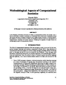
Figure 2.8: Discrepancy of Pseudorandom Numbers (PRN) and Quasirandom Numbers (QRN) for d = 2 and d = 3 We used a Linear Congruential Generator (LCG) to provide the pseudorandom numbers and we used a Sobol’ sequence to produce the quasirandom numbers. In Figure 2.8, as N grows, the slope of the log/log graph of the discrepancy of the pseudorandom numbers is close to –1/2, fitting the theoretical trend of O(N-1/2). The slope of the discrepancy of the quasirandom numbers is similarly close to –1, again confirming the theory.

Table 2.1: Performance of Exact Algorithm Computing the Discrepancy d=2 N 4 8 16 32 64 128 256 CPU Time(s) 0.0019 0.0029 0.0047 0.0088 0.0146 0.0351 0.0820 N 512 1024 2048 4096 8192 16384 32768 CPU Time(s) 0.1865 0.4726 1.9394 11.617 38.53 59.90 482.11 Table 2.2: Performance of Exact Algorithm Computing the Discrepancy d=3 N 4 8 16 32 64 128 256 CPU Time(s) 0.0029 0.0046 0.0068 0.0136 0.0419 0.1767 1.1601 N 512 1024 2048 4096 CPU Time(s) 15.705 165.88 2354.8 83097

19

Table 2.1 and 2.2 show the performance of the exact algorithm. As N or d grows, the computation time grows rapidly. In an experiment for N = 1000 and d = 7, the exact computation takes several weeks on an Alpha-class machine to obtain the exact discrepancy. If N or d is too large, the exact algorithm is impractical, even with the algorithmic improvements previously described.

Note: All of the numerical results were computed on a DEC Alpha DS10 6/466 with 256M of DRAM. 20

CHAPTER 3 AN APPROXIMATE ALGORITHM FOR COMPUTING DN*

3.1

Introduction

The problem of exactly evaluating DN* of a given point set, as described in the previous chapter, leads to a large-scale integer computation problem. Although the method based on orthants and the improved N-to-1 method can reduce the number of enumerations, with large N or d, the algorithm is still impractical. As no other exact algorithm is known requiring only a reasonable amount of computing resources for large d and N, the use of optimization heuristics to this algorithm seems appropriate.

Winker and Fang [7] gave an approximate algorithm using a threshold-accepting method. However, their numerical results seem not to be satisfactory, especially when the dimension d is large, the speed of the threshold-accepting method is too slow. Thiémard [10] provided an algorithm for computing the upper bound for star discrepancy. The algorithm runs in O(N*d*logk+2d*kd) time and O(kd) space, where k > 1 is an arbitrary integer. However, “the larger k, the better the bound gets, but the more time and memory are required for its computation.” Especially when d is large, the computation with this algorithm will become very costly.

The “curse of dimensionality” bears its ugly head in evaluating the discrepancy. This gives us a hint. Can we use the Monte Carlo method, the only viable method for a 21

wide range of high-dimensional problems, to evaluate the discrepancy of a point set? This motivates us to consider a Monte Carlo algorithm based on random walks to approximately estimate DN* .

3.2

The Approximate Algorithm Using Random Walks

3.2.1 Random Walks As we stated previously, the evaluation of DN* reduces to the procedure of finding the maximum discrepancy among the grid points in the unit cube. Hence, we could generate random walks on these grid points to sample points to find their maximum. The random walk is relatively simple here. Every walk starts at the origin. There will be d possible directions at every step to find the next grid point in the randomly chosen direction. The random walk stops when it reaches the border of the unit cube Id. Figure 3.1 presents the paths of some random walks in a two-dimensional case. The algorithm computes the discrepancy at every grid point on the random path to estimate the maximum discrepancy.

Figure 3.1: 3 Random Walks on the Grid At this time, we obtain the maximum discrepancy of the grid points encountered by all of the random walks and the location of the maximum. It is very possible to find a grid point around the current point that has a larger discrepancy. Thus, we might create 22

an expanded search by searching the grid points around the current maximum to find another possible maximum.

3.2.2 Implementation Algorithm 3.1 implements the approximate algorithm using random walks to compute the DN* discrepancy. m is the number of random walks.

Algorithm 3.1 [Random Walks] [Initialization] [1] For every dimension i from 1 to d Sort x0, …, xN-1 by their i-th coordinates, respectively, together with 0 and 1. [Random Walk] [2] For realizations from 1 to m Start from origin Repeat Randomly select one direction from d directions Go to the next grid point in the selected direction Compute the discrepancy at the grid point If it is bigger than the current maximum discrepancy, mark down location of the grid point and set the maximum discrepancy Until reach the border of the unit cube

[Expanded Searching] [3] Get the available grid point has the current maximum discrepancy. Repeat Search all of the 2d grid points around the current grid point for larger discrepancy 23

If such a grid point available, mark down location of the grid point as the current grid point and set the maximum discrepancy Until no grid points around the current point has a larger discrepancy.

[4] Set the maximum discrepancy as the overall discrepancy

This algorithm is relatively easy to implement. The maximum length of a random walk is N*d, and the complexity of the algorithm using random walks is O(N*d*m), where m is the number of realizations of random walks. The data structure is also simple. We only need to store the grid point with current maximum discrepancy, so the storage needed is only O(1).

3.2.3 Numerical Results Figure 3.2 compares the exact computation and the approximate computation in three-dimensional pseudorandom sequences. When the number of points is small, the approximate method based on random walks fits the exact solution quite well. When the number of points increases, the approximation begins to deviate from the exact solution. Using more realizations of random walks can eliminate the deviation.

24

Figure 3.2: The Random Walk Approximation Method of Computing the Discrepancy Versus N

Figure 3.3: The Random Walk Approximation Method of Computing the Discrepancy Versus Dimension The convergence rate of the approximation method seriously affects its efficiency. Figures 3.3 gives the convergence of the approximation method when using 1,000 and 10,000 random walks, for dimension 2 through 8. The experimental experience suggests that the convergence rate of the method based on random walks is better for large d and small N than the case of large N and small d. 25

Figure 3.4: Convergence of the Random Walk Approximation Method Versus Increasing Number of Random Walks m Figure 3.4 shows that with more random walks, the result of the method based on random walks converges to the exact value. In the numerical experiments, computing the discrepancy of 100 7-dimensional quasirandom points, it took the exact computing algorithm one week to obtain the exact solution. Using 105 random walks, the approximation method spent 25.3 seconds to find the approximate result, which is 0.129 and is close to the exact value of 0.136. 106 random walks continue to improve the approximate result to 0.133 in 247.8 seconds. However, sometimes the convergence rate is very slow. When we compute 100 8-dimensional quasirandom numbers, the exact value is 0.160794. The approximate value changes from 0.151225 to 0.153533 while we vary the random walks from 10 5 to 107. Note, by definition, the approximate results we obtain are always lower bounds for the exact results. Thus we know that as the number of random walks used increases, we will monotonically approach the exact value. This monotonic convergence could be used with extrapolation to further speed our approximation.

26

Table 3.1: Performance of Random Walk Algorithm Computing the Discrepancy d = 2, 1000 random walks N 512 1024 2048 4096 8192 16384 32768 CPU Time (s) 0.72 1.47 2.92 5.78 11.54 23.22 46.34 Table 3.2: Performance of Random Walk Algorithm Computing the Discrepancy N = 100, 1000 random walks d 2 3 4 5 6 7 8 CPU Time (s) 0.186 0.297 0.422 0.575 0.723 0.900 1.11 Table 3.3: Performance of Random Walk Algorithm Computing the Discrepancy d = 8, N = 100 Random Walks 100 1,000 10,000 100,000 1,000,000 CPU Time (s) 0.110 1.11 11.18 119.9 1098.67 Table 3.1, 3.2 and 3.3 show the performance of the random walk algorithm. The computation time grows linearly, as N, d or the number of random walks m grows.

3.2.4 Discussion The approximate algorithm using random walks gives a lower bound of the star discrepancy DN*. The advantage of the random walk algorithm is that it is easy to implement and its time and space complexities are much smaller than the exact algorithms. Therefore, we can estimate the discrepancy of a random sequence in high dimension with the approximation algorithm with only a fraction of the CPU time required by the exact algorithm. In addition, it is very easy to implement the approximate algorithm on a parallel computer, as it is a Monte Carlo method. For instance, we can easily divide the approximate computation of discrepancy into smaller tasks and submit them to the parallel High-Throughput Condor Computing system [12], which will finally significantly reduce the total computation time. In order to estimate the discrepancy of sequences with very large N, we are implementing a parallel approximate algorithm based on random walks, which divides the point set into smaller portions and

27

simultaneously estimate the discrepancy of points occurring in several random walks in each smaller portion.

However, the limitation of the approximate method is that it is hard to estimate the error between the exact discrepancy and the discrepancy computed by the approximate algorithm. Since the random walk method is based on the method of Monte Carlo search, the convergence rate of the method should also be the same as Monte Carlo search, i.e., O(N-1/2) [8] [10] [11]. Perhaps an effective method of extrapolation with N can improve this. In addition, if we use quasi-Monte Carlo search instead of Monte Carlo search, the convergence rate may likewise be improved.

28

CHAPTER 4 COMPUTING THE L2 DISCREPANCY In the previous two chapters, we discussed the exact algorithm and an approximate algorithm for computing the star discrepancy in the L ∞ norm. In this chapter, we discuss the computation of the star discrepancy in the L2 norm. Fortunately, there is an explicit formula available for computing the L2 discrepancy. The time and space requirements for computing L2 discrepancy are thus not as costly as that of the L∞ discrepancy.

4.1

The Formula for Computing the L2 Discrepancy

There is a directly computable formula for computing the L2 discrepancy, TN* [7]. TN* = [ ∫ d RN ( J (0, t )) 2 dt ]1/ 2 I

= [ ∫ d ( µ X ( J ) − µ ( J )) 2 dt1 ...dt d ]1/ 2 I

d

= [ ∫ d (∏ t k ) 2 dt1...dt d − I

k =1

= [3−d −

1− d

2 N

N

d

d 2 N 1 t x ( k ) dt1...dt d + 2 ∑ d ∏ k i ∫ N i =1 I k =1 N

∑∏ (1 − ( x i =1 k =1

) )+

(k ) 2 i

1 N2

N

d

N

∑∫ ∏x

i , j =1

Id

(k ) i

x (jk ) dt1...dt d ]1 / 2 .

k =1

d

∑∏ (1 − max( x

i , j =1 k =1

(k ) i

, x (jk ) ))]1/ 2

Here, xj(k) stands for the k-th dimensional value of the j-th point in the random number sequence.

29

4.2

The Algorithm for Computing L2 Discrepancy

By using the above formula, we can obtain a straightforward computation of the L2 discrepancy. The computation of the second term of the formula requires O(N*d) time while the computation of the third term requires O(N2*d) time. Heinrich [7] gave an efficient algorithm for computing the third term with an average-case complexity of O(N*d*(logN)d), which finally improves the total cost of computing the L2 discrepancy to O(N*d*(logN)d).

4.3

Numerical Results

Figure 4.1: Numerical Results of L2 Discrepancy By using the formula for computing the L2 discrepancy, we obtained numerical results similar to those for the discrepancy using L∞ norm. Figure 4.1 shows that as N grows, the slope of the L2 discrepancy of pseudorandom numbers is close to –1/2, obeying the theoretical trend of O(N-1/2). Similarly, the slope of the L2 discrepancy of quasirandom numbers is near –1. 30

It is important to note that the cost of computing the L2 star discrepancy, TN* is much less than the cost of computing the exact L∞ discrepancy DN*, as shown in Table 4.1 and Table 4.2. Comparing Table 4.1 to the performance of computing the L∞ discrepancy of the same point set shown in Table 2.2, the computation of the L∞ discrepancy takes 83097 seconds of CPU time while that of the L2 discrepancy only requires 1.63 seconds! Therefore, to analyze the quality of the quasirandom number sequences, using the L2 discrepancy to measure the uniformity seems to be more appropriate than using the L∞ discrepancy. They both provide similar results, but the L2 discrepancy is so much cheaper to compute.

Table 4.1: Performance of Algorithm of Computing L2 Discrepancy d=3 N 4 8 16 32 64 128 CPU Time 0.000002 0.000008 0.00003 0.00007 0.0002 0.00098 N 512 1024 2048 4096 8192 16384 CPU Time 0.0175 0.0840 0.275 1.63 6.71 26.6

256 0.00391 32768 105.7

Table 4.2: Performance of Algorithm of Computing L2 Discrepancy N = 1000 d 2 3 4 5 6 7 CPU Time (s) 0.0625 0.0752 0.119 0.140 0.157 0.177 d 9 10 11 12 13 14 CPU Time (s) 0.230 0.260 0.273 0.325 0.329 0.349

8 0.206 15 0.411

4.4

Approximation Method for the L2 Discrepancy

Exactly computing the L2 discrepancy, TN*, is easier than computing DN*. Since TN* is an integral, there may be a way to use a Monte Carlo integration method to approximately estimate the L2 discrepancy. With deeper analysis, however, this seems to be more complicated than original thought. For an arbitrary hyper-rectangle, J, in the unit cube, Id, it is easy to compute the 31

volume, µ(J), of J, but hard to compute the discrete measure, µX(J), of J. This is because we must examine all of the points to count the number of points in J: this is a very costly operation, and unlike the orthant algorithm, one cannot amortize the cost of computing

µX(J) over many related computations. To reduce to cost of computing µX(J), we tried a method of estimating only a portion of the point set, e.g., 106 points out of 109 points. This fraction of points was randomly selected. The cost of evaluating the µX(J) is reduced, however, our computational experiments indicate that many more iterations are required for convergence of the approximate result. The total improvement of this method is not significant and not as efficient as the exact method based on the formula.

Our own computational experience shows that crude Monte Carlo estimation of *

the TN is slower than the exact formula. However, more work is required to see if either optimization, or algorithmic restructuring will yield a viable approximate algorithm. Another possible approach is the use of approximation to the exact formula for TN* to obtain faster approximate estimates.

32

CHAPTER 5 APPLICATION OF DISCREPANCY COMPUTATION ALGORITHMS A discrepancy computation algorithm can be used to evaluate the uniformity of a sequence of numbers. It can be used to test the discrepancy of different quasirandom number generators and provide error bound estimates for quasi-Monte Carlo integration and simulation via the Koksma-Hlawka inequality. In addition, these algorithms can be used to empirically distinguish between good and better quasirandom sequences. Thus they will be useful in choosing optimal parameters for an “optimal” high dimensional quasirandom number generator. In Figure 5.1, we use the exact computation to estimate the star discrepancy DN* and TN* of a two-dimensional Sobol’ sequence, Halton’ sequence and Faure’ sequence [15]. As shown in Figure 5.2, we use the approximation algorithm using random walks to analyze the approximate star discrepancies, DN*, of the above quasirandom sequences, with d ranging from 2 to 14. Our computational experiments show that the Sobol’ sequence has a better uniformity than the other two sequences in this case.

33

Figure 5.1 DN* and TN* of Sobol’ Sequence, Halton’ Sequence and Faure’ Sequence

Figure 5.2 Approximate Algorithm Using Random Walks to Estimate Discrepancies of Sobol’ sequence, Halton’ sequence and Faure’ sequence

In [13], we used a quasi-Monte Carlo method to solve an elliptic boundary value problem. If we try to apply quasirandom numbers to the Markov chain method employed, a high dimensional quasirandom sequence is required. However, a very high dimensional quasirandom sequence is hard to obtain. If we try to construct a multi-dimensional quasirandom sequence via one-dimensional quasirandom sequences, and use the discrepancy computation algorithm to estimate the uniformity of the constructed 34

sequence, we found that the discrepancy of this constructed sequence is too large and not appropriate for use in this case.

Currently, we have a code for generating a 40-dimensional Sobol’ sequence [15]. However, in practical quasi-Monte Carlo computations and simulations, we often need a higher dimensional Sobol’ sequence, e.g. a 360-dimensional Sobol’ sequence is required to simulate a 30-year mortgage backed security. When we try to extend this sequence to higher dimensions, we can use the approximate algorithm of computing the discrepancy to generate an optimal high dimensional Sobol’ sequence.

35

CHAPTER 6 SUMMARY 6.1

Conclusion

We discussed using discrepancy to measure the uniformity of random sequences. Exact computation methods and approximate methods for star discrepancy, DN*, and the formula for computing the L2 discrepancy are presented. We also discussed some applications of computing the discrepancy.

The exact computation method for star discrepancy in the L∞ norm is costly in both time and space. When estimating the quasi-Monte Carlo integration error bound or the quality of quasirandom number sequences, it can be used only when d and N are small. If d or N are large, the exact computation method becomes impractical. However, the computation of L2 discrepancy is relatively cheap and it can be used to analyze the quality of quasirandom number sequences as effectively as the L∞ method, when d or N are larger. However, if d or N are very large, we can only use the approximate random walk method or the computation of the discrepancy bound [10] to estimate the uniformity of sequences. If we can find a better way to use Monte Carlo method to estimate the L2 discrepancy, we may use it in this case, too.

Figure 6.1 compares the CPU time required when using different methods to estimate DN* or TN*.

36

Figure 6.1: Comparison of CPU Time of Different Methods

6.2

Future Work

In the future, we hope to work on the following problems related. 1. We plan to more carefully examine the complexity of the 1-to-N versus the N-to1 orthant algorithm. 37

2. We hope to extend the concept of the measure of uniformity. The measure of uniformity we discussed here is only defined on the unit cube. Some applications need to use uniformity on spheres or other objects. Our future work will be into a wider definition of measures of uniformity and algorithms for its efficient numerical estimation. 3. We plan to devise a fast approximate algorithm to improve the performance of computing the L2 discrepancy. 4. Extrapolation of discrepancies with small N or d to estimate the discrepancy of large N or high d deserves further research. 5. In order to generate the “good” high dimensional Sobol’ sequences, we plan to apply the methods to measure uniformity to a search protocol to adjust the generation parameters to generate a high dimensional Sobol’ sequence. 6. We plan to carefully analyze the appropriateness of the described algorithms to parallel computation. We then hope to implement optimized version of these for use in item 4. 7. Using the implementation of the algorithms for computing the discrepancy, we plan to implement a quasi-Monte Carlo integration program, which will provide an approximate Koksma-Hlawka error bound. 8. Accelerate the computation of exact discrepancy DN* by using quasi-Monte Carlo search. 9. We plan to carefully analyze the approximate random walk algorithm for computing DN* and analyze approximate DN*.

38

REFERENCES [1] “Random Number Generation and Quasi-Monte Carlo Methods,” H. Niederreiter, SIAM CBMS-NSF Regional Conference Series in Applied Mathematics, Philadelphia, PA, 1992. [2] “Monte Carlo and Quasi-Monte Carlo Methods,” Russel E. Caflisch, Acta Numerica, pp. 1-49, 1998. [3] “Computing the Discrepancy,” D. Dobkin and D. Eppstein, Proceedings of the Ninth Annual Symposium on Computational Geometry, pp. 47-52, 1993. [4] “A Method for Exact Calculation of the Star-Discrepancy of Plane Sets Applied to the Sequences of Hammersley,” L. De Clerk, Mh. Math., 101:261-278, 1986. [5] “A Method for Exact Calculation of the Discrepancy of Low-Dimensional Finite Point Set,” P. Bundschuh and Y. C. Zhu, Abh. Math. Sem. Univ. Hamburg, 63:115-133, 1993. [6] “Application of threshold-accepting to the evaluation of the discrepancy of a set of points,” Peter Winker and Kai-Tai Fang, SIAM Journal Number Anal., 34:2028-2042, 1997. [7] “Efficient Algorithms for Computing the L2-Discrepancy,” S.Heinrich, Mathematics of Computation, 65:1621-1633, 1996. [8] “On the Assessment of Random and Quasirandom Point Sets,” Peter Hellekalek, Lecture Notes in Statistics. Eds., Vol. 138, 1998. [9] “An Algorithm to Compute Bounds for the Star Discrepancy,” Eric Thiémard, Journal of Complexity, 1999. [10] “Uniform Random Number Generation,” Pierre, L’ecuyer, Annals of Operations Research, 1994.

39

[11] “Generating Quasirandom Paths for Stochastic Processes,” William J. Morokoff, SIAM Rev., 40:765-788, 1998. [12] “Condor - A Hunter of Idle Workstations,” M. Litzkow, M. Livny, and M. W. Mutka, Proceedings of the 8th International Conference of Distributed Computing Systems, pp. 104-111, 1988. [13] “Quasi-Monte Carlo method for elliptic boundary value problems,” Michael Mascagni, Aneta Karaivanova, Yaohang Li, preprint, Int. Conf. On Monte Carlo and Prob. Methods for PDE, Monaco, 2000. [14] “SPRNG: A Scalable Library for Pseudorandom Number Generation,” Michael Mascangi, Ashok Svinuasan, ACM Transactions on Mathematical Software, in the press, 2000. [15] “Quasirandom sequence generator for multivariate quadrature and optimization,” P. Bratley and B. L. Fox, Collected Algorithms From ACM Transactions on Mathematical Software, 14:88-100, 1988. [16] “Monte Carlo Principles and Neutron Transport Problems,” J. Spanier and E. M. Gelbard, Addison-Wesley, Reading, Massachusetts, 1969. [17] “Monte Carlo Methodologies and Applications for Pricing and Risk Management,” Bruno Dupire, Risk Publications, 1999.

40

BIOGRAPHICAL SKETCH The Author was born in Guangzhou, China on Sept. 22, 1974. He attended the South China University of Technology, Guangzhou, China and got his B.A. in Computer Science and Engineering in July 1997. He worked for IBM China Limited as a Software and Networking Information Technology Specialist from 1997 to 1998. Since August 1998, he spent a year in the Ph.D. program of Scientific Computing in University of Southern Mississippi. In 1999, he transferred to the Department of Computer Science at Florida State University. After the Master’s degree, the author is going to continue to pursue his Ph.D. degree in Computer Science at Florida State University.

41