The Continuous Genetic Algorithm

CHAPTER 3

The Continuous Genetic Algorithm

Now that you are convinced (perhaps) that the binary GA solves many optimization problems that stump traditional techniques, let’s look a bit closer at the quantization limitation. What if you are attempting to solve a problem where the values of the variables are continuous and you want to know them to the full machine precision? In such a problem each variable requires many bits to represent it. If the number of variables is large, the size of the chromosome is also large. Of course, 1s and 0s are not the only way to represent a variable. One could, in principle, use any representation conceivable for encoding the variables. When the variables are naturally quantized, the binary GA fits nicely. However, when the variables are continuous, it is more logical to represent them by floating-point numbers. In addition, since the binary GA has its precision limited by the binary representation of variables, using floating point numbers instead easily allows representation to the machine precision. This continuous GA also has the advantage of requiring less storage than the binary GA because a single floating-point number represents the variable instead of Nbits integers. The continuous GA is inherently faster than the binary GA, because the chromosomes do not have to be decoded prior to the evaluation of the cost function. The purpose of this chapter is to introduce the continuous GA. Most sources call this version of the GA a real-valued GA. We use the term continuous rather than real-valued to avoid confusion between real and complex numbers. The development here closely parallels the last chapter. We primarily dwell upon the differences in the two algorithms. The continuous example introduced in Chapter 1 is our primary example problem. This allows the reader to compare the continuous GA performance with the more traditional optimization algorithms introduced in Chapter 1.

Practical Genetic Algorithms, Second Edition, by Randy L. Haupt and Sue Ellen Haupt. ISBN 0-471-45565-2 Copyright © 2004 John Wiley & Sons, Inc.

51

52

THE CONTINUOUS GENETIC ALGORITHM

Define cost function, cost, variables Select GA parameters

Generate initial population

Find cost for each chromosome

Select mates

Mating

Mutation

Convergence Check

done

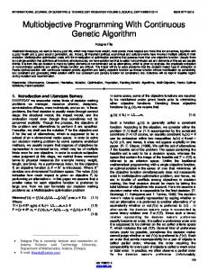
Figure 3.1

3.1

Flowchart of a continuous GA.

COMPONENTS OF A CONTINUOUS GENETIC ALGORITHM

The flowchart in Figure 3.1 provides a “big picture” overview of a continuous GA. Each block is discussed in detail in this chapter. This GA is very similar to the binary GA presented in the last chapter. The primary difference is the fact that variables are no longer represented by bits of zeros and ones, but instead by floating-point numbers over whatever range is deemed appropriate. However, this simple fact adds some nuances to the application of the technique that must be carefully considered. In particular, we will present different crossover and mutation operators. 3.1.1

The Example Variables and Cost Function

As we saw in the last chapter, the goal is to solve some optimization problem where we search for an optimal (minimum) solution in terms of the variables of the problem. Therefore we begin the process of fitting it to a GA by defining a chromosome as an array of variable values to be optimized. If the chromosome has Nvar variables (an N-dimensional optimization problem) given by p1, p2, . . . , pN var then the chromosome is written as an array with 1 ¥ Nvar elements so that


chromosome = [ p1, p2 , p3 , . . . , pN var ]

53

(3.1)

In this case, the variable values are represented as floating-point numbers. Each chromosome has a cost found by evaluating the cost function f at the variables p1, p2, . . . , pN var . cost = f (chromosome) = f ( p1, p2 , . . . , pN var )

(3.2)

Equations (3.1) and (3.2) along with applicable constraints constitute the problem to be solved. Our primary example in this chapter is the continuous function introduced in Chapter 1. Consider the cost function cost = f ( x, y) = x sin(4 x) + 1.1y sin(2 y)

(3.3)

Subject to the constraints: 0 £ x £ 10 and 0 £ y £ 10 Since f is a function of x and y only, the clear choice for the variables is chromosome = [ x, y]

(3.4)

with Nvar = 2. A contour map of the cost function appears as Figure 1.4. This cost function is considerably more complex than the cost function in Chapter 2. We see that peaks and valleys dot the landscape of the cost function contour plot. The plethora of local minima overwhelms traditional minimum-seeking methods. Our goal is to find the global minimum value of f(x, y).

3.1.2

Variable Encoding, Precision, and Bounds

Here is where we begin to see the differences from the prior chapter. We no longer need to consider how many bits are necessary to accurately represent a value. Instead, x and y have continuous values that fall between the bounds listed in equation (3.3). Although the values are continuous, a digital computer represents numbers by a finite number of bits. When we refer to the continuous GA, we mean the computer uses its internal precision and roundoff to define the precision of the value. Now the algorithm is limited in precision to the roundoff error of the computer. Since the GA is a search technique, it must be limited to exploring a reasonable region of variable space. Sometimes this is done by imposing a constraint on the problem such as equation (3.3). If one does not know the initial search region, there must be enough diversity in the initial population to explore a reasonably sized variable space before focusing on the most promising regions.

54


3.1.3

Initial Population

To begin the GA, we define an initial population of Npop chromosomes. A matrix represents the population with each row in the matrix being a 1 ¥ Nvar array (chromosome) of continuous values. Given an initial population of Npop chromosomes, the full matrix of Npop ¥ Nvar random values is generated by pop = rand(Npop, Nvar) All variables are normalized to have values between 0 and 1, the range of a uniform random number generator. The values of a variable are “unnormalized” in the cost function. If the range of values is between plo and phi, then the unnormalized values are given by p = ( phi - plo ) pnorm + plo

(3.5)

where plo

= highest number in the variable range

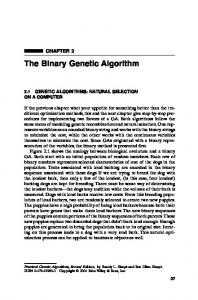
phi = lowest number in the variable range pnorm = normalized value of variable In our example, the unnormalized values are just 10pnorm. This society of chromosomes is not a democracy: the individual chromosomes are not all created equal. Each one’s worth is assessed by the cost function. So at this point, the chromosomes are passed to the cost function for evaluation. We begin solving (3.3) by filling a Npop ¥ Nvar matrix with uniform random numbers between 0 and 10. Figure 3.2 shows the initial random population for the Npop = 8 chromosomes. Population values are listed in Table 3.1. We see widely scattered population members that well sample the values of the cost function. None of the initial guesses are particularly close to the global minimum. 3.1.4

Natural Selection

Now is the time to decide which chromosomes in the initial population are fit enough to survive and possibly reproduce offspring in the next generation. As done for the binary version of the algorithm, the Npop costs and associated chromosomes are ranked from lowest cost to highest cost. The rest die off. This process of natural selection must occur at each iteration of the algorithm to allow the population of chromosomes to evolve over the generations to the most fit members as defined by the cost function. Not all of the survivors are deemed fit enough to mate. Of the Npop chromosomes in a given generation, only the top Nkeep are kept for mating and the rest are discarded to make room for the new offspring.


55

Figure 3.2 Contour plot of the cost function with the initial population (Npop = 8) indicated by large dots.

TABLE 3.1 Example Initial Population of 8 Random Chromosomes and Their Corresponding Cost x 6.9745 0.30359 2.402 0.18758 2.6974 5.613 7.7246 6.8537

y

Cost

0.8342 9.6828 9.3359 8.9371 6.2647 0.1289 5.5655 9.8784

3.4766 5.5408 -2.2528 -8.0108 -2.8957 -2.4601 -9.8884 13.752

TABLE 3.2 Surviving Chromosomes after a 50% Selection Rate Number 1 2 3 4

x

y

Cost

7.7246 0.1876 2.6974 5.6130

5.5655 8.9371 6.2647 0.12885

-9.8884 -8.0108 -2.8957 -2.4601

In our example the mean of the cost function for the population of 8 was -0.3423 and the best cost was -9.8884. After discarding the bottom half the mean of the population is -5.8138. The natural selection results represented to five significant digits are shown in Table 3.2.

56


TABLE 3.3 Pairing and Mating Process of SinglePoint Crossover Chromosome Family Binary String Cost

3.1.5

2

ma(1)

0.18758

8.9371

3

pa(1)

2.6974

6.2647

5

offspring1

0.2558

6.2647

6

offspring2

2.6292

8.9371

3

ma(2)

2.6974

6.2647

1

pa(2)

7.7246

5.5655

7

offspring3

6.6676

5.5655

8

offspring4

3.7544

6.2647

Pairing

The Nkeep = 4 most-fit chromosomes form the mating pool. Two mothers and fathers pair in some random fashion. Each pair produces two offspring that contain traits from each parent. In addition the parents survive to be part of the next generation. The more similar the two parents, the more likely are the offspring to carry the traits of the parents. We presented some basic approaches to finding two mates in Chapter 2 and refer the reader back to that presentation rather than repeating it. The example presented here uses rank weighting with the probabilities shown in Table 2.5. A random number generator produced the following two pairs of random numbers: (0.6710, 0.8124) and (0.7930, 0.3039). Using these random pairs and Table 2.5, the following chromosomes were randomly selected to mate: ma = [2 3] pa = [3 1] Thus chromosome2 mates with chromosome3, and so forth. The ma and pa vectors contain the numbers corresponding to the chromosomes selected for mating. Table 3.3 summarizes the results. 3.1.6

Mating

As for the binary algorithm, two parents are chosen, and the offspring are some combination of these parents. Many different approaches have been tried for crossing over in continuous GAs. Adewuya (1996) reviews some of the methods. Several interesting methods are demonstrated by Michalewicz (1994).


57

The simplest methods choose one or more points in the chromosome to mark as the crossover points. Then the variables between these points are merely swapped between the two parents. For example purposes, consider the two parents to be parent1 = [ pm 1 , pm 2 , pm 3 , pm 4 , pm 5 , pm 6 , . . . , pmN var ] parent 2 = [ pd 1 , pd 2 , pd 3 , pd 4 , pd 5 , pd 6 , . . . , pdN var ]

(3.6)

Crossover points are randomly selected, and then the variables in between are exchanged: offspring1 = [ pm 1 , pm 2 , ≠ pd 3 , pd 4 , ≠ pm 5 , pm 6 , . . . , pmN var ] offspring 2 = [ pd 1 , pd 2 , ≠ pm 3 , pm 4 , ≠ pd 5 , pd 6 , . . . , pdN var ]

(3.7)

The extreme case is selecting Nvar points and randomly choosing which of the two parents will contribute its variable at each position. Thus one goes down the line of the chromosomes and, at each variable, randomly chooses whether or not to swap information between the two parents. This method is called uniform crossover: offspring1 = [ pm 1 , pd 2 , pd 3 , pd 4 , pd 5 , pm 6 , . . . , pdN var ] offspring 2 = [ pd 1 , pm 2 , pm 3 , pm 4 , pm 5 , pd 6 , . . . , pmN var ]

(3.8)

The problem with these point crossover methods is that no new information is introduced: each continuous value that was randomly initiated in the initial population is propagated to the next generation, only in different combinations. Although this strategy worked fine for binary representations, there is now a continuum of values, and in this continuum we are merely interchanging two data points. These approaches totally rely on mutation to introduce new genetic material. The blending methods remedy this problem by finding ways to combine variable values from the two parents into new variable values in the offspring. A single offspring variable value, pnew, comes from a combination of the two corresponding offspring variable values (Radcliff, 1991) pnew = b pmn + (1 - b ) pdn where b = random number on the interval [0, 1] pmn = nth variable in the mother chromosome pdn = nth variable in the father chromosome

(3.9)

58


The same variable of the second offspring is merely the complement of the first (i.e., replacing b by 1 - b). If b = 1, then pmn propagates in its entirety and pdn dies. In contrast, if b = 0, then pdn propagates in its entirety and pmn dies. When b = 0.5 (Davis, 1991), the result is an average of the variables of the two parents. This method is demonstrated to work well on several interesting problems by Michalewicz (1994). Choosing which variables to blend is the next issue. Sometimes, this linear combination process is done for all variables to the right or to the left of some crossover point. Any number of points can be chosen to blend, up to Nvar values where all variables are linear combinations of those of the two parents. The variables can be blended by using the same b for each variable or by choosing different b’s for each variable. These blending methods effectively combine the information from the two parents and choose values of the variables between the values bracketed by the parents; however, they do not allow introduction of values beyond the extremes already represented in the population. To do this requires an extrapolating method. The simplest of these methods is linear crossover (Wright, 1991). In this case three offspring are generated from the two parents by pnew1 = 0.5 pmn + 0.5 pdn pnew 2 = 1.5 pmn - 0.5 pdn pnew 3 = -0.5 pmn + 1.5 pdn

(3.10)

Any variable outside the bounds is discarded in favor of the other two. Then the best two offspring are chosen to propagate. Of course, the factor 0.5 is not the only one that can be used in such a method. Heuristic crossover (Michalewicz, 1991) is a variation where some random number, b, is chosen on the interval [0, 1] and the variables of the offspring are defined by pnew = b ( pmn - pdn ) + pmn

(3.11)

Variations on this theme include choosing any number of variables to modify and generating different b for each variable. This method also allows generation of offspring outside of the values of the two parent variables. Sometimes values are generated outside of the allowed range. If this happens, the offspring is discarded and the algorithm tries another b. The blend crossover (BLX-a) method (Eshelman and Shaffer, 1993) begins by choosing some parameter a that determines the distance outside the bounds of the two parent variables that the offspring variable may lie. This method allows new values outside of the range of the parents without letting the algorithm stray too far. Many codes combine the various methods to use the strengths of each. New methods, such as quadratic crossover (Adewuya, 1996), do a numerical fit to the fitness function. Three parents are necessary to perform a quadratic fit. The algorithm used in this book is a combination of an extrapolation method with a crossover method. We wanted to find a way to closely


59

mimic the advantages of the binary GA mating scheme. It begins by randomly selecting a variable in the first pair of parents to be the crossover point a = roundup{random * N var }

(3.12)

We’ll let parent1 = [ pm 1 pm 2 K pma K pmN var ] parent 2 = [ pd 1 pd 2 K pda K pdN var ]

(3.13)

where the m and d subscripts discriminate between the mom and the dad parent. Then the selected variables are combined to form new variables that will appear in the children: pnew1 = pma - b [ pma - pda ] pnew 2 = pda + b [ pma - pda ]

(3.14)

where b is also a random value between 0 and 1. The final step is to complete the crossover with the rest of the chromosome as before: offspring1 = [ pm 1 pm 2 K pnew1 K pdN var ] offspring 2 = [ pd 1 pd 2 K pnew 2 K pmN var ]

(3.15)

If the first variable of the chromosomes is selected, then only the variables to the right of the selected variable are swapped. If the last variable of the chromosomes is selected, then only the variables to the left of the selected variable are swapped. This method does not allow offspring variables outside the bounds set by the parent unless b > 1. For our example problem, the first set of parents are given by chromosome2 = [0.1876, 8.9371] chromosome3 = [2.6974, 6.2647] A random number generator selects p1 as the location of the crossover. The random number selected for b is b = 0.0272. The new offspring are given by offspring1 = [0.18758 - 0.0272 ¥ 0.18758 + 0.0272 ¥ 2.6974, 6.2647] = [0.2558, 6.2647] offspring 2 = [2.6974 + 0.0272 ¥ 0.18758 - 0.0272 ¥ 2.6974, 8.9371] = [2.6292, 8.9371]

60


Continuing this process once more with a b = 0.7898. The new offspring are given by offspring3 = [2.6974 - 0.7898 ¥ 2.6974 + 0.7898 ¥ 7.7246, 6.2647] = [6.6676, 5.5655] offspring4 = [7.7246 + 0.7898 ¥ 2.6974 - 0.7898 ¥ 7.7246, 8.9371] = [3.7544, 6.2647]

3.1.7

Mutations

Here, as in the last chapter, we can sometimes find our method working too well. If care is not taken, the GA can converge too quickly into one region of the cost surface. If this area is in the region of the global minimum, that is good. However, some functions, such as the one we are modeling, have many local minima. If we do nothing to solve this tendency to converge quickly, we could end up in a local rather than a global minimum. To avoid this problem of overly fast convergence, we force the routine to explore other areas of the cost surface by randomly introducing changes, or mutations, in some of the variables. For the binary GA, this amounted to just changing a bit from a 0 to a 1, and vice versa. The basic method of mutation is not much more complicated for the continuous GA. For more complicated methods, see Michalewicz (1994). As with the binary GA, we chose a mutation rate of 20%. Multiplying the mutation rate by the total number of variables that can be mutated in the population gives 0.20 ¥ 7 ¥ 2 3 mutations. Next random numbers are chosen to select the row and columns of the variables to be mutated. A mutated variable is replaced by a new random variable. The following pairs were randomly selected: mrow = [4 4 7] mcol = [1 2 1] The first random pair is (4, 1). Thus the value in row 4 and column 1 of the population matrix is replaced with a uniform random number between one and ten: 5.6130 ﬁ 9.8190 Mutations occur two more times. The first two columns in Table 3.4 show the population after mating. The next two columns display the population after mutation. Associated costs after the mutations appear in the last column. The mutated values in Table 3.4 appear in italics. Note that the first chromosome


TABLE 3.4

Mutating the Population

Population after Mating

Population after Mutations

x

y

x

y

cost

5.5655 8.9371 6.2647 0.12885 6.2647 8.9371 5.5655 6.2647

7.7246 0.18758 2.6974 9.819 0.2558 2.6292 9.1602 3.7544

5.5655 8.9371 6.2647 7.1315 6.2647 8.9371 5.5655 6.2647

-9.8884 -8.0108 -2.8957 17.601 -0.03688 -10.472 -14.05 2.1359

7.7246 0.18758 2.6974 5.613 0.2558 2.6292 6.6676 3.7544

61

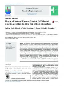
Figure 3.3 Contour plot of the cost function with the population after the first generation.

is not mutated due to elitism. The mean for this population is -3.202. The third offspring (row 7) has the best cost due to the crossover and mutation. If the x-value were not mutated, then the chromosome would have a cost of 0.6 and would have been eliminated in the natural selection process. Figure 3.3 shows the distribution of chromosomes after the first generation. Most users of the continuous GA add a normally distributed random number to the variable selected for mutation pn¢ = pn + sN n (0, 1) where s = standard deviation of the normal distribution Nn(0, 1) = standard normal distribution (mean = 0 and variance = 1)

(3.6)

62


We do not use this technique because a good value for s must be chosen, the addition of the random number can cause the variable to exceed its bounds, and it takes more computer time.

3.1.8

The Next Generation

The process described is iterated until an acceptable solution is found. For our example, the starting population for the next generation is shown in Table 3.5 after ranking. The bottom four chromosomes are discarded and replaced by offspring from the top four parents. Another three random variables are selected for mutation from the bottom 7 chromosomes. The population at the end of generation 2 is shown in Table 3.6 and Figure 3.4. Table 3.7 is the ranked population at the beginning of generation 3. After mating, mutation, and ranking, the final population after three generations is shown in Table 3.8 and Figure 3.5.

TABLE 3.5 New Ranked Population at the Start of the Second Generation x 9.1602 2.6292 7.7246 0.18758 2.6974 0.2558 3.7544 9.819

y

Cost

5.5655 8.9371 5.5655 8.9371 6.2647 6.2647 6.2647 7.1315

-14.05 -10.472 -9.8884 -8.0108 -2.8957 -0.03688 2.1359 17.601

TABLE 3.6 Population after Crossover and Mutation in the Second Generation x 9.1602 2.6292 7.7246 0.18758 2.6292 9.1602 7.7246 4.4042

y

Cost

5.5655 8.9371 6.4764 8.9371 5.8134 8.6892 8.6806 7.969

-14.05 -10.472 -1.1376 -8.0108 -7.496 -17.494 -13.339 -6.1528


63

TABLE 3.7 New Ranked Population at the Start of the Third Generation x 9.1602 9.1602 7.7246 2.6292 0.18758 2.6292 4.4042 7.7246

TABLE 3.8 Most Cost x 9.0215 9.1602 9.1602 9.1602 9.1602 2.6292 7.7246 7.8633

y

Cost

8.6892 5.5655 8.6806 8.9371 8.9371 5.8134 7.969 6.4764

-17.494 -14.05 -13.339 -10.472 -8.0108 -7.496 -6.1528 -1.137

Ranking of Generation 3 from Least to y

Cost

8.6806 8.6892 8.323 5.5655 8.1917 8.9371 1.8372 3.995

-18.53 -17.494 -15.366 -14.05 -13.618 -10.472 -4.849 4.6471

Figure 3.4 Contour plot of the cost function with the population after the second generation.

64


Figure 3.5 Contour plot of the cost function with the population after the third and final generation.

0

population average

cost

-5

-10

best

-15

-20

0

1

2

3

generation

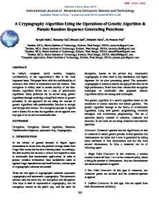
Figure 3.6 Plot of the minimum and mean costs as a function of generation. The algorithm converged in three generations.

3.1.9

Convergence

This run of the algorithm found the minimum cost (-18.53) in three generations. Members of the population are shown as large dots on the cost surface contour plot in Figures 3.2 to 3.5. By the end of the second generation, chromosomes are in the basins of the four lowest minima on the cost surface. The global minimum of -18.5 is found in generation 3. All but two of the population members are in the valley of the global minimum in the final generation. Figure 3.6 is a plot of the mean and minimum cost for each generation. The GA was able to find the global minimum, unlike the Nelder-Mead and BFGS algorithms presented in Chapter 1.

EXERCISES

3.2

65

A PARTING LOOK

The binary GA could have been used in this example as well as a continuous GA. Since the problem used continuous variables, it seemed more natural to use the continuous GA. The next chapter presents some practical optimization problems for both the binary and continuous GAs. Selecting the various GA parameters, such as mutation rate and type of crossover, is still more of an art than a science and will be discussed in Chapter 5.

BIBLIOGRAPHY Adewuya, A. A. 1996. New methods in genetic search with real-valued chromosomes. Master’s thesis. Massachusetts Institute of Technology, Cambridge. Davis, L. 1991. Hybridization and numerical representation. In L. Davis (ed.), The Handbook of Genetic Algorithms. New York: Van Nostrand Reinhold, pp. 61–71. Eshelman, L. J., and D. J. Shaffer. 1993. Real-coded genetic algorithms and intervalschemata. In D. L. Whitley (ed.), Foundations of Genetic Algorithms 2. San Mateo, CA: Morgan Kaufman, pp. 187–202. Michalewicz, Z. 1994. Genetic Algorithms + Data Structures = Evolution Programs, 2nd ed. New York: Springer-Verlag. Radcliff, N. J. 1991. Forma analysis and random respectful recombination. In Proc. 4th Int. Conf. on Genetic Algorithms, San Mateo, CA: Morgan Kauffman. Wright, A. 1991. Genetic algorithms for real parameter optimization. In G. J. E. Rawlins (ed.), Foundations of Genetic Algorithms. San Mateo, CA: Morgan Kaufmann, pp. 205–218.

EXERCISES 1. Write a continuous GA that uses the following crossover: a. b. c. d. e.

(3.7) (3.8) (3.9) (3.10) (3.14)

2. Write a continuous GA that uses: a. b. c. d. e.

Pairing parents from top to bottom Random pairing Pairing based on cost Roulette wheel rank weighting Tournament selection

66


3. Find the minimum of _____ (from Appendix I) using your continuous GA. 4. Experiment with different population sizes and mutation rates. Which combination seems to work best for you? Explain. 5. Compare your GA with one of the following local optimizers: a. b. c. d. e.

Nelder-Mead downhill simplex BFGS DFP Steepest descent Random search

6. Since the GA has many random components, it is important to average the results of several runs. Write a program that will average the results of several GA runs. Now, do another one of the exercises and compare results. 7. Plot the convergence of the GA. Which GA parameters have the most effect on convergence? 8. Compare the performance of the binary and continuous GAs. Which do you prefer and why? Does the type of problem make a difference?